There are two sources that I would like to acknowledge here. This dataset was used in a research paper published by Moro and others: A data-driven approach to predict the success of bank telemarketing, Decision support systems, Elsevier, June 2014. Later on, it was donated to the UCI Machine Learning Repository, which can be downloaded from https://archive.ics.uci.edu/ml/datasets/bank+marketing.

According to the dataset description, there are four datasets:

There are 21 attributes in the dataset. The independent variables can be further categorized as bank-client-related data (attributes 1 to 7), related to the last contact from the current campaign (attributes 8 to 11). Other attributes (attributes 12 to 15), and social and economic context attributes (attributes 16 to 20) are categorized. The dependent variable is specified by y, the last attribute (21):

You can see that the dataset is not ready to feed to your MLP, or DBN classifier, directly since the feature is mixed with numerical and categorical values. In addition, the outcome variable is in categorical value. Therefore, we need to convert the categorical values into numerical values, so that the feature and the outcome variable are in numerical form. The next step shows this process. Refer to the preprocessing_b.py file for this preprocessing.

Firstly, we must load the required packages and libraries needed for the preprocessing:

import pandas as pd
import numpy as np
from sklearn import preprocessing

Then download the data file from the aforementioned URL and place it in your convenient place – say input:

Then, we load and parse the dataset:

data = pd.read_csv('input/bank-additional-full.csv', sep = ";")

Next, we'll extract variable names:

var_names = data.columns.tolist()

Now, based on the dataset description in Table 1, we'll extract the categorical variables:

categs = ['job','marital','education','default','housing','loan','contact','month','day_of_week','duration','poutcome','y']

Then, we'll extract the quantitative variables:

# Quantitative vars
quantit = [i for i in var_names if i not in categs]

Then let's get the dummy variables for categorical variables:

job = pd.get_dummies(data['job'])
marital = pd.get_dummies(data['marital'])
education = pd.get_dummies(data['education'])
default = pd.get_dummies(data['default'])
housing = pd.get_dummies(data['housing'])
loan = pd.get_dummies(data['loan'])
contact = pd.get_dummies(data['contact'])
month = pd.get_dummies(data['month'])
day = pd.get_dummies(data['day_of_week'])
duration = pd.get_dummies(data['duration'])
poutcome = pd.get_dummies(data['poutcome'])

Now, it's time to map variables to predict:

dict_map = dict()
y_map = {'yes':1,'no':0}
dict_map['y'] = y_map
data = data.replace(dict_map)
label = data['y']
df_numerical = data[quantit]
df_names = df_numerical .keys().tolist()

Once we have converted the categorical variables into numerical variables, the next task is to normalize the numerical variables too. So, using the normalization, we scale an individual sample to have unit norm. This process can be useful if you plan to use a quadratic form such as the dot product, or any other kernel, to quantify the similarity of any pair of samples. This assumption is the basis of the vector space model (https://en.wikipedia.org/wiki/Vector_space_model) often used in text classification and clustering contexts.

So, let's scale the quantitative variables:

min_max_scaler = preprocessing.MinMaxScaler()
x_scaled = min_max_scaler.fit_transform(df_numerical)
df_temp = pd.DataFrame(x_scaled)
df_temp.columns = df_names

Now that we have the temporary data frame for the (original) numerical variables, the next task is to combine all the data frames together and generate the normalized data frame. We will use pandas for this:

normalized_df = pd.concat([df_temp,
                      job,
                      marital,
                      education,
                      default,
                      housing,
                      loan,
                      contact,
                      month,
                      day,
                      poutcome,
                      duration,
                      label], axis=1)

Finally, we need to save the resulting data frame in a CSV file as follows:

normalized_df.to_csv('bank_normalized.csv', index = False)

For this example, we will be using the bank marketing dataset that we have normalized in the previous example. There are several steps to follow. To begin with, we need to import TensorFlow, and the other necessary packages and modules:

import tensorflow as tf
import pandas as pd
import numpy as np
import os
from sklearn.cross_validation import train_test_split # for random split of train/test

Now, we need to load the normalized bank marketing dataset, where all the features and the labels are numeric. For this we use the read_csv() method from the pandas library:

FILE_PATH = 'bank_normalized.csv'         # Path to .csv dataset 
raw_data = pd.read_csv(FILE_PATH)        # Open raw .csv
print("Raw data loaded successfully...
")

The following is the output of the preceding code:

>>>
Raw data loaded successfully...

As mentioned in the previous section, tuning the hyperparameters for DNNs is not straightforward. However, it often depends on the dataset that you are handling. For some datasets, a possible workaround is setting these values based on dataset-related statistics, for example, the number of training instances, the input size, and the number of classes.

DNNs are not suitable for very small and low-dimensional datasets. In these cases, a better option is to use the linear models instead. To get started, let us put a pointer to the label column itself, compute the number of instances and number of classes, and define the train/test split ratio as follows:

Y_LABEL = 'y'    # Name of the variable to be predicted
KEYS = [i for i in raw_data.keys().tolist() if i != Y_LABEL]# Name of predictors
N_INSTANCES = raw_data.shape[0]       # Number of instances
N_INPUT = raw_data.shape[1] - 1            # Input size
N_CLASSES = raw_data[Y_LABEL].unique().shape[0] # Number of classes
TEST_SIZE = 0.25         # Test set size (% of dataset)
TRAIN_SIZE = int(N_INSTANCES * (1 - TEST_SIZE))  # Train size

Now, let's see the statistics of the dataset that we are going to use to train the MLP model:

print("Variables loaded successfully...
")
print("Number of predictors 	%s" %(N_INPUT))
print("Number of classes 	%s" %(N_CLASSES))
print("Number of instances 	%s" %(N_INSTANCES))
print("
")

The following is the output of the preceding code:

>>>
Variables loaded successfully...
Number of predictors     1606
Number of classes          2
Number of instances      41188

The next task is to define the other parameters such as learning rate, training epochs, batch size, and the standard deviation for the weights. Usually, a low value of training rate will help your DNN to learn more slowly, but intensively. Note that we need to define more parameters, such as the number of hidden layers, and the activation function.

LEARNING_RATE = 0.001     # learning rate
TRAINING_EPOCHS = 1000     # number of training epoch for the forward pass
BATCH_SIZE = 100     # batch size to be used during training
DISPLAY_STEP = 20   # print the error etc. at each 20 step
HIDDEN_SIZE = 256   # number of neurons in each hidden layer
# We use tanh as the activation function, but you can try using ReLU as well
ACTIVATION_FUNCTION_OUT = tf.nn.tanh
STDDEV = 0.1        # Standard Deviations
RANDOM_STATE = 100

The preceding initialization is set on a trial-and-error basis. Therefore, depending on your use case and data types, set them wisely but we will provide some guidelines later in this chapter. In addition, for the preceding code, RANDOM_STATE is used to signify random state for the train and test split. At first, we separate the raw features and the labels:

data = raw_data[KEYS].get_values()       # X data
labels = raw_data[Y_LABEL].get_values()  # y data

Now that we have the labels, they have to be coded:

labels_ = np.zeros((N_INSTANCES, N_CLASSES))
labels_[np.arange(N_INSTANCES), labels] = 1

Finally, we must split the training and test sets. As mentioned earlier, we'll keep 75% of the input for training and the remaining 25% for the test set:

data_train, data_test, labels_train, labels_test = train_test_split(data,labels_,test_size = TEST_SIZE,random_state = RANDOM_STATE)
print("Data loaded and splitted successfully...
")

The following is the output of the preceding code:

>>>
Data loaded and splitted successfully

Since this is a supervised classification problem, we should have placeholders for the features and the labels:

As mentioned previously, an MLP is composed of one input layer, several hidden layers, and one final layer of LTUs called the output layer. For this example, I am going to incorporate the training with four hidden layers. Thus, we are calling our classifier a deep feed-forward MLP. Note that we also need to have the weight in each layer (except in the input layer), and the bias in each layer (except the output layer). Usually, each hidden layer includes a bias neuron, and is fully connected to the next layer as a fully-connected bipartite graph (feed-forward) from one hidden layer to another. So, let's define the size of the hidden layers:

n_input = N_INPUT                   # input n labels 
n_hidden_1 = HIDDEN_SIZE            # 1st layer 
n_hidden_2 = HIDDEN_SIZE            # 2nd layer
n_hidden_3 = HIDDEN_SIZE            # 3rd layer 
n_hidden_4 = HIDDEN_SIZE            # 4th layer 
n_classes = N_CLASSES               # output m classes 

Since this is a supervised classification problem, we should have placeholders for the features and the labels:

# input shape is None * number of input
X = tf.placeholder(tf.float32, [None, n_input])

The first dimension of the placeholder is None, meaning we can have any number of rows. The second dimension is fixed at number of features, meaning each row needs to have that number of columns of features.

# label shape is None * number of classes
y = tf.placeholder(tf.float32, [None, n_classes])

Additionally, we need another placeholder for dropout, which is implemented by only keeping a neuron active with some probability (say p < 1.0, or setting it to zero otherwise). Note that this is also hyperparameters to be tuned and the training time, but not the test time:

dropout_keep_prob = tf.placeholder(tf.float32)

Using the scaling given here enables the same network to be used for training (with dropout_keep_prob < 1.0) and evaluation (with dropout_keep_prob == 1.0). Now, we can define a method that implements the MLP classifier. For this, we are going to provide four parameters such as input, weight, biases, and the drop out probability as follows:

def DeepMLPClassifier(_X, _weights, _biases, dropout_keep_prob):
    layer1 = tf.nn.dropout(tf.nn.tanh(tf.add(tf.matmul(_X, _weights['h1']), _biases['b1'])), dropout_keep_prob)
    layer2 = tf.nn.dropout(tf.nn.tanh(tf.add(tf.matmul(layer1, _weights['h2']), _biases['b2'])), dropout_keep_prob)
    layer3 = tf.nn.dropout(tf.nn.tanh(tf.add(tf.matmul(layer2, _weights['h3']), _biases['b3'])), dropout_keep_prob)
    layer4 = tf.nn.dropout(tf.nn.tanh(tf.add(tf.matmul(layer3, _weights['h4']), _biases['b4'])), dropout_keep_prob)
    out = ACTIVATION_FUNCTION_OUT(tf.add(tf.matmul(layer4, _weights['out']), _biases['out']))
return out

The return value of the preceding method is the output of the activation function. The preceding method is a stub implementation that did not tell anything concrete about the weights and biases, so before we start the training, we should have them defined:

weights = {
    'w1': tf.Variable(tf.random_normal([n_input, n_hidden_1],stddev=STDDEV)),
    'w2': tf.Variable(tf.random_normal([n_hidden_1, n_hidden_2],stddev=STDDEV)),
    'w3': tf.Variable(tf.random_normal([n_hidden_2, n_hidden_3],stddev=STDDEV)),
    'w4': tf.Variable(tf.random_normal([n_hidden_3, n_hidden_4],stddev=STDDEV)),
    'out': tf.Variable(tf.random_normal([n_hidden_4, n_classes],stddev=STDDEV)),   
}
biases = { 
    'b1': tf.Variable(tf.random_normal([n_hidden_1])), 
    'b2': tf.Variable(tf.random_normal([n_hidden_2])), 
    'b3': tf.Variable(tf.random_normal([n_hidden_3])), 
    'b4': tf.Variable(tf.random_normal([n_hidden_4])), 
    'out': tf.Variable(tf.random_normal([n_classes])) 
}

Now we can invoke the preceding implementation of the MLP with real arguments (an input layer, weights, biases, and the drop out) keeping probability as follows:

pred = DeepMLPClassifier(X, weights, biases, dropout_keep_prob)

We have built the MLP model and it's time to train the network itself. At first, we need to define the cost op and then we will use Adam optimizer, which will learn slowly and try to reduce the training loss as much as possible:

cost = tf.reduce_mean(tf.nn.softmax_cross_entropy_with_logits_v2(logits=pred, labels=y))

# Optimization op (backprop)
optimizer = tf.train.AdamOptimizer(learning_rate = LEARNING_RATE).minimize(cost_op)

Next, we need to define additional parameters for computing the classification accuracy:

correct_prediction = tf.equal(tf.argmax(pred, 1), tf.argmax(y, 1))
accuracy = tf.reduce_mean(tf.cast(correct_prediction, tf.float32))
print("Deep MLP networks has been built successfully...")
print("Starting training...")

After that, we need to initialize all the variables and placeholders, before launching a TensorFlow session:

init_op = tf.global_variables_initializer() 

Now, we are very closer to starting the training, but before that, the last step is to create a TensorFlow session and launch it as follows:

sess = tf.Session()
sess.run(init_op)

Finally, we are ready to start training our MLP on the training set. We iterate over all the batches and fit using the batched data to compute the average training cost. Nevertheless, it would be great to show the training cost and accuracy for each epoch:

for epoch in range(TRAINING_EPOCHS):
    avg_cost = 0.0
    total_batch = int(data_train.shape[0] / BATCH_SIZE)
    # Loop over all batches
    for i in range(total_batch):
        randidx = np.random.randint(int(TRAIN_SIZE), size = BATCH_SIZE)
        batch_xs = data_train[randidx, :]
        batch_ys = labels_train[randidx, :]
        # Fit using batched data
        sess.run(optimizer, feed_dict={X: batch_xs, y: batch_ys, dropout_keep_prob: 0.9})
        # Calculate average cost
        avg_cost += sess.run(cost, feed_dict={X: batch_xs, y: batch_ys, dropout_keep_prob:1.})/total_batch
    # Display progress
    if epoch % DISPLAY_STEP == 0:
        print("Epoch: %3d/%3d cost: %.9f" % (epoch, TRAINING_EPOCHS, avg_cost))
        train_acc = sess.run(accuracy, feed_dict={X: batch_xs, y: batch_ys, dropout_keep_prob:1.})
        print("Training accuracy: %.3f" % (train_acc))
print("Your MLP model has been trained successfully.")

Following is the output of the preceding code:

>>>
Starting training...
Epoch:   0/1000 cost: 0.356494816
Training accuracy: 0.920
…
Epoch: 180/1000 cost: 0.350044933
Training accuracy: 0.860
….
Epoch: 980/1000 cost: 0.358226758
Training accuracy: 0.910

Well done, our MLP model has been trained successfully! Now, what if we see the cost and the accuracy graphically? Let's try it out:

# Plot loss over time
plt.subplot(221)
plt.plot(i_data, cost_list, 'k--', label='Training loss', linewidth=1.0)
plt.title('Cross entropy loss per iteration')
plt.xlabel('Iteration')
plt.ylabel('Cross entropy loss')
plt.legend(loc='upper right')
                   plt.grid(True)

Following is the output of the preceding code:

>>>

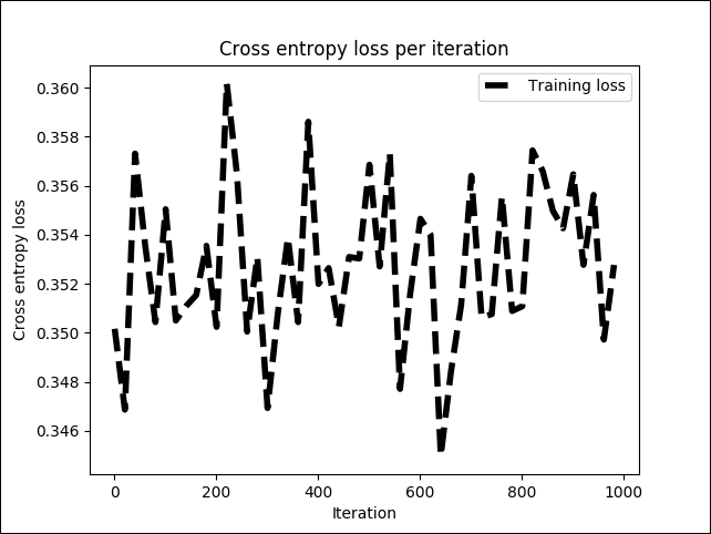
Figure 11: Cross entropy loss per iteration in the training phase

The preceding figure shows that the cross-entropy loss is more or less stable between 0.34 and 0.36, but with a little fluctuation. Now, let's see how this affects the training accuracy overall:

# Plot train and test accuracy
plt.subplot(222)
plt.plot(i_data, acc_list, 'r--', label='Accuracy on the training set', linewidth=1.0)
plt.title('Accuracy on the training set')
plt.xlabel('Iteration')
plt.ylabel('Accuracy')
plt.legend(loc='upper right')
plt.grid(True)
plt.show()

Following is the output of the preceding code:

>>>

Figure 12: Accuracy on the training set on each iteration

We can see that the training accuracy fluctuates between 79% and 96% but does not increase or decrease uniformly. One possible way around this is to add more hidden layers and use different optimizers, such as gradient descent, which was discussed earlier in this chapter. We will increase the dropout probability to 100%, that is, 1.0. The reason is to have the same network used for testing as well:

print("Evaluating MLP on the test set...")
test_acc = sess.run(accuracy, feed_dict={X: data_test, y: labels_test, dropout_keep_prob:1.})
print ("Prediction/classification accuracy: %.3f" % (test_acc))

Following is the output of the preceding code:

>>>
Evaluating MLP on the test set...
Prediction/classification accuracy: 0.889
Session closed!

Thus, the classification accuracy is about 89%. Not bad at all! Now, if higher accuracy is desired, we can use another architecture of DNNs called Deep Belief Networks (DBNs), that can be trained either in a supervised or unsupervised way.

This is the easiest way to observe DBN in its application as a classifier. If we have a DBN classifier, then the pre-training method is done in an unsupervised way similar to an autoencoder which will be described in Chapter 5, Optimizing TensorFlow Autoencoders and the classifier is trained (fine-tuned) in a supervised way, exactly like the one in MLP.

An RBM is an undirected probabilistic graphical model called Markov random fields. It consists of two layers. The first layer is composed of visible neurons and second layer consist of hidden neurons. Figure 14 shows the structure of a simple RBM. Visible units accept inputs, and hidden units are nonlinear feature detectors. Each visible neuron is connected to all the hidden neurons, but there is no internal connection among neurons in the same layer:

Figure 14: The structure of a simple RBM

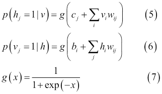
The RBM in Figure 14 consists of m visible units, V = (v₁ ,…v_m ) and n hidden units, H = (h₁ …h_n ). Visible units accept values between 0 and 1 and generated values of hidden units are between 0 and 1. The joint probability of the model is an energy function given by the following equation:

In the preceding equation, i = 1…m, j = 1…n, b i, and c j are biases of visible and hidden units respectively, and w _ij is the weight between v _i and _hj. The probability assigned by the model to a visible vector v is given by the following equation:

In the second equation, Z is a partition function defined as follows:

The learning of weight can be attained by the following equation:

In equation 4, the learning rate is defined by . In general, a smaller value of ensures that training is more intensive. However, if you want your network to learn quickly, you can set this value higher.

It is easy to calculate the first term since there are no connections among units in the same layer. Conditional distributions of p(h|v) and p(v|h) are factorial, and given by the logistic function in the following equations:

Hence, the sample v _ih _j is unbiased. However, calculating the log-likelihood of the second term is exponentially expensive to compute. Although it is possible to get unbiased samples of the second term, using Gibbs sampling by running Markov Chain Monte Carlo (MCMC), this process is not cost-effective either. Instead, RBM uses an efficient approximation method called contrastive divergence.

In general, MCMC requires many sampling steps to reach convergence to stationary. Running Gibbs sampling for few steps (usually one) is enough to train a model, which is called contrastive divergence learning. The first step of contrastive divergence is to initialize the visible units with a training vector.

The next step is to compute all hidden units, using visible units at the same time, with equation five, then reconstruct visible units from hidden units using equation four. Lastly, the hidden units are updated with the reconstructed visible units. Therefore, instead of equation four, we get the following weight-learning model in the end:

In short, this process tries to reduce the reconstruction error between input data and reconstructed data. Several iterations of parameter update are required for the algorithm to converge. Iterations are called epoch. Input data is divided into mini batches, and parameters are updated after each mini batch, with the average values of the parameters.

Finally, as stated earlier, RBM maximizes the probability of visible units p(v), which is defined by the mode and overall training data. It is equivalent to minimizing the KL-divergence (https://en.wikipedia.org/wiki/Kullback%E2%80%93Leibler_divergence) between the model distribution and the empirical data distribution.

Contrastive divergence is only a crude approximation of this objective function, but it works very well in practice. Although it is convenient, the reconstruction error is actually a very poor measure of the progress of learning. Considering these aspects, RBM requires some time to converge, but if you see that the reconstruction is decent, then your algorithm works well.

A single hidden layer RBM cannot extract all the features from the input data, due to its inability to model the relationship between variables. Hence, multiple layers of RBMs are used one after another to extract non-linear features. In DBNs, an RBM is trained first with input data, and the hidden layer represents learned features in a greedy learning approach.

These learned features of the first RBM are used as the input of the second RBM, as another layer in the DBN, which is shown in Figure 15. Similarly, learned features of the second layer are used as input for another layer.

This way, DBNs can extract deep and non-linear features from input data. The hidden layer of the last RBM represents the learned features of the whole network. The process of learning features, described earlier for all RBM layers, is called pre-training.

Suppose you want to tackle a complex task, for which you do not have much-labeled training data. It will be difficult to find a suitable DNN implementation, or architecture, to be trained and used for predictive analytics. Nevertheless, if you have plenty of unlabeled training data, you can try to train the layers one by one, starting with the lowest layer and then going up, using an unsupervised feature detector algorithm. This is how exactly RBMs (Figure 15) or autoencoders (Figure 16) work.

Figure 15: Unsupervised pre-training in a DBN using autoencoders

Unsupervised pre-training is still a good option when you have a complex task to solve, no similar model you can reuse, and little-labeled training data, but plenty of unlabeled training data. The current trend is using autoencoders rather than RBMs; however, for the example in the next section, RBMs will be used for simplicity. Readers can also try using autoencoders rather than RBMs.

Pre-training is an unsupervised learning process. After pre-training, fine-tuning of the network is carried out, by adding a labeled layer at the top of the last RBM layer. This step is a supervised learning process. The unsupervised pre-training step tries to find network weights:

Figure 16: Unsupervised pre-training in a DBN by constructing a simple a DBN with a stack of RBMs

In the supervised learning stage (also called supervised fine-tuning), instead of randomly initializing network weights, they are initialized with the weights computed in the pre-training step. This way, DBNs can avoid converging to a local minimum when a supervised gradient descent is used.

As stated earlier, using a stack of RBMs, a DBN can be constructed as follows:

Therefore, putting these steps together, Figure 17 shows the construction of a simple DBN, consisting of three RBMs:

Figure 17: Construction of a simple DBN using several RBMs

Now, when it comes to tuning a DBN for better predictive accuracy, we should tune several hyper-parameters, so that DBNs fit the training data by untying and refining W ². Putting this all together, we have the conceptual workflow for creating a DBN-based classifier or regressor.

Now that we have enough theoretical background on how to construct a DBN using several RBMs, it is time to apply our theory in practice. In the next section, we will see how to develop a supervised DBN classifier for predictive analytics.