
3
Artificial Intelligence Models
3.1. Introduction
Artificial intelligence (AI) is a branch of computer science with the aim of making machines capable of reasoning and perception. This overall objective is pursued through both practical and theoretical routes. In practice, the aim is to make machines capable of performing tasks which require intelligence as handled by a human. In theory, people want to pursue a scientific understanding of the computational principles underlying intelligent behavior, as manifested in humans and other animals. Both routes need to propose and understand operational principles of thought and action in computational terms. These principles may form the foundations of computer implementations of thought and action and, if suitably grounded in experimental method, may in some ways contribute to explanations of human thought and behavior.
AI research has been applied in broad ways. For instance, computer programs play chess at an expert level, assess insurance and credit risks, automatically identify objects from images, and search the contents of the Internet. From the scientific perspective, however, the aim of understanding intelligence from a computational point of view remains elusive. As an example, current programs for automatic reasoning can prove useful theorems concerning the correctness of large-scale digital circuitry, but exhibit little or no common sense. Current language-processing programs can translate simple sentences into database queries, but the programs are misled by the kind of idioms, metaphors, conversational ploys or ungrammatical expressions that we take for granted. Current vision programs can recognize a simple set of human faces in standard poses, but are misled by changes of illumination, or natural changes in facial expression and pose, or changes in cosmetics, spectacles or hairstyle. Current knowledge-based medical-expert systems can diagnose an infectious disease and prescribe an antibiotic therapy but, if you describe your motor car to the system, it will tell you what kind of meningitis your car has; the system does not know that cars do not get diseases. Current learning systems can forecast financial trends, given historical data, but cannot predict the date of Easter nor prime numbers given a large set of examples.
Inspired by the capacities of the human brain, AI-based models integrate the specific attributes of various disciplines, such as mathematics, physics, computer science and, recently, environmental engineering applications. AI-based prediction models have a significant potential for solving complex environmental applications that include large amounts of independent parameters and nonlinear relationships. Because of their predictive capabilities and nonlinear characteristics, several AI-based modeling techniques, such as artificial neural networks, fuzzy logic and adaptive neuro-fuzzy inference systems, have recently been conducted in the modeling of various real-life processes in the energy engineering field.
In this chapter, the basis of two widely used AI-based techniques, namely artificial neural networks and support vector machines, is theoretically summarized and important mathematical aspects of these methods are highlighted. Moreover, computational issues, and respective advantages of these methods are described.
3.2. Artificial neural networks
In the human brain, neurons are connected as a network to implement intelligent control and thinking. Inspired by this biological structure, an artificial neural network was proposed for supervised learning. The word “artificial” indicates it is a mathematical model, and it differs from a brain neural network. A typical neural network consists of an interconnected group of artificial neurons, and it contains information using a connection list approach to computation. Modern neural networks are nonlinear statistical data modeling tools. They are usually used to model complex relationships between inputs and outputs or to find patterns in data. Let us introduce this computational model, starting from the basic element and the simplest structure.
3.2.1. Single-layer perceptron
Figure 3.1(a) shows the basic computational element of a neural network which is often called a node or a neuron. It receives input Ii from some other units, or perhaps from an external source. Each input Ii has an associated weight wi, which can be modified so as to train the model. Each neuron is composed of two units. The first unit adds products of weight coefficients and input signals. The second unit realizes the nonlinear function, called neuron activation function, i.e. f(.). The output of this neuron is denoted by y:

Its output y, in turn, can serve as an input to other units. The whole network consists of a topology graph of neurons, each of which computes an activation function of the inputs carried on the in-edges and sends the output on its out-edges. The inputs and outputs are weighed by weights wij and shifted by a bias factor specific to each neuron.
Figure 3.1(b) gives the simplest neural network example which contains a single output layer. Inputs are fed directly to the output via a series of weights, no other hidden neurons exist. This structure is called a single-layer perceptron.
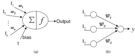
Figure 3.1. Example of one neuron a) and a single-layer perceptron b)
In this simple neural network, the sum of the products of the weights and inputs is calculated in each node, i.e. ![]() . For example, if the value of the output is above a certain threshold t, the neuron takes the activated value, otherwise it takes the deactivated value. It can be formulated as follows:
. For example, if the value of the output is above a certain threshold t, the neuron takes the activated value, otherwise it takes the deactivated value. It can be formulated as follows:

Neurons with this kind of activation function are also called artificial neurons or linear threshold units. In the literature, the term “perceptron” often refers to networks consisting of just one of these units. A perceptron can be created using any value for the activated and deactivated states as long as the threshold value lies between the two. Typically, the output of most perceptrons is either 1 or -1 with a threshold equal to 0.
Perceptrons can be trained by a simple learning algorithm that is usually called the delta rule. It calculates the errors between estimated output and sample output data, and uses this to create an adjustment to the weights, thus implementing a form of gradient descent. For a neuron j, with activation function f(x), the delta rule for j’s ith weight wji, is given by:
where α is a small constant called learning rate, f(x) is the neuron’s activation function, tj is the jth target output, hj is the summation of inputs ![]() is the actual output yi = f(hj), xi is the ith input.
is the actual output yi = f(hj), xi is the ith input.
It is very important to choose an appropriate activation function for each neuron. Usually, all neurons in a specific network share the same function. The common choices are:
- – identity, i.e. f(x) = x;
- – sigmoid, i.e.
 , also known as logistic function;
 - – tanh, i.e.
- – step, i.e.

Single-unit perceptrons are limited in performance. They are only capable of learning linearly separable patterns. For example, the simple, yet classic XOR function cannot be solved by a single-layer perceptron network since we cannot find a linear hyperplane to separate these two classes.
3.2.2. Feed forward neural network
The above single-layer perceptron is exactly a simple example of a feed forward neural network. In a feed forward network, the information transfers forward from input nodes, through hidden nodes (if any) to the output nodes, in only one direction. There are no cycles or loops in the network. The common feed forward network is a multi-layer perceptron (MLP) which contains one or more layers of hidden neurons, as shown in Figure 3.2. The neurons in the hidden layers are not directly accessible.

Figure 3.2. Feed forward neural network
The training of an MLP is usually accomplished by using a back-propagation algorithm which involves two steps. Suppose that we have chosen the network’s structure, activation function, and that free parameters for each node are initialized, then the forward step and the backward step are defined as follows: adjustments (see equation [3.3]) are applied to the free parameters of each neuron so as to minimize the squared estimation error.
- – forward step: during this phase, the free parameters of the network, including weights and bias, are fixed, and the input signal is propagated through the network layer-by-layer. The output of the previous node is fed as input to the next node. The equation is the same as [3.1]. The forward phase finishes with the computation of an error signal ei = |ti − yi| where yi is the estimated target in response to the input xi and ti is the actual sample target;
- – backward step: the error signal ei is propagated through the network in the backward direction, also layer-by-layer. It is during this phase that
There are two basic ways to implement back-propagation learning, namely the batch mode and the online mode:
- – batch mode: in this mode, adjustments are made to the free parameters of the network on an epoch-by-epoch basis, where each epoch consists of the entire set of training examples. The batch mode is best suited for nonlinear regression;
- – online mode (or sequential mode): in this mode of back-propagation learning, adjustments are made to the free parameters of the network on an example-by-example basis. This mode is suited for pattern classification.
The advantage of a back-propagation learning algorithm is that it is simple to implement and computationally efficient due to the fact that its complexity is linear in the synaptic weights of the network. However, a major limitation of this algorithm is that the convergence is not always guaranteed and can be excruciatingly slow, particularly when the network topology is large.
There are many ways that feed forward neural networks can be constructed. Besides input and output layers, we must consider how many hidden layers we should have, and how many neurons in each layer. Using too few neurons in the hidden layers will result in under fitting which further leads to insufficient detection ability of the model on the signals in a complicated dataset. In contrast, using too many neurons in the hidden layers can result in several problems. First, it might cause an overfitting problem which leads to poor generalization ability on testing datasets. The second problem is the training time which will increase since the topology complexity is high. Neural networks with two hidden layers can represent functions with any kind of shape. Currently, there is no theoretical reason to use neural networks with more than two hidden layers for many practical problems. Some experiments are required to determine the optimal structure for the feed forward neural network. Readers can refer to [REE 99] for more details.
3.2.3. Radial basis functions network
Another popular layered feed forward network is the radial basis function (RBF) network. It has important properties of universal approximation. It is a paradigm of neural networks, which was developed considerably later than that of perceptrons. Like perceptrons, the RBF networks have a layered structure, which is composed of exactly three layers, i.e. only a single layer of hidden neurons. A simple example of this type of neural network is shown in Figure 3.3.

Figure 3.3. Simple radial basis functions neural network architecture
For each layer, it has the following properties:
- – input layer: there is only one neuron in the input layer for each predictor variable. In the case of categorical variables, N − 1 neurons are used where N represents the number of categories. The input neurons (or processing before the input layer) standardize the range of values by subtracting the median and dividing by the interquartile range. The input neurons then feed the values to each of the neurons in the hidden layer;
- – hidden layer: this layer has a variable number of neurons (the optimal number is determined by the training process). Each neuron consists of a radial basis function centered on a point with as many dimensions as there are predictor variables. The activation function is given by:

where X is the input feature vector, L is the number of hidden neurons, μj and ∑j are the mean and the covariance matrix of the jth Gaussian function. The spread (radius) of the RBF function may be different for each dimension. The centers and spreads are determined by the training process. When presented with the x vector of input values from the input layer, a hidden neuron computes the Euclidean distance of the test case from the neuron’s center point and then applies the RBF kernel function to this distance using the spread values. The resulting value is passed to the summation layer;
- – output layer: the value coming out of a neuron in the hidden layer is multiplied by a weight associated with the neuron (W1, W2, … , Wn in this figure) and passed to the summation which adds up the weighted values and presents this sum as the output of the network, as follows:

In other words, the output neurons contain only the identity function. For classification problems, there is one output (and a separate set of weights and summation unit) for each target category. The value output for a category is the probability that the case being evaluated has that category.
RBF networks differ from multilayer perceptrons in the following fundamental respects. The former consists of local approximators, whereas the latter consists of global approximators. The former has a single hidden layer, whereas the latter can have any number of hidden layers. The output layer of an RBF network is always linear, whereas in a multilayer perceptron it can be either linear or nonlinear. The activation function of the hidden layer in an RBF network computes the Euclidean distance between the input signal vector and parameter vector of the network, whereas the activation function of a multilayer perceptron computes the inner product between the input signal vector and the pertinent synaptic weight vector.
When training RBF networks, the following parameters are determined:
- – the number of neurons in the hidden layer;
- – the coordinates of the center of each hidden-layer RBF function;
- – the radius (spread) of each RBF function in each dimension;
- – the weights applied to the RBF function outputs as they are passed to the summation layer.
RBF networks use memory-based learning for their design. Specifically, the summation on the output neuron means learning can be viewed as a curve-fitting problem in high-dimensional space.
A large variety of methods have been used to train RBF networks. One of them uses K-means clustering to find cluster centers which are then used as the centers for the RBF functions. However, K-means clustering is a computationally intensive procedure, and it often does not generate the optimal number of centers. Another common approach is to use a random subset of the training points as the centers.
3.2.4. Recurrent neural network
Recurrent neural networks (RNNs) differ in a fundamental way from feed forward architectures in the sense that they not only operate on an input space but also on an internal state space, a trace of what has already been processed by the network. Figure 3.4 shows a simple example where nodes s retain internal states, weights w2 are recurrent weights. This additional layer is also called a “context” layer. At each time step, new inputs are fed into the RNN. The previous contents of the hidden layer are copied into the context layer. These are then fed back into the hidden layer in the next time step. The network recurrently influences itself by including the output in the following computation steps.

Figure 3.4. Simple recurrent neural network
There are various types of recurrent networks of nearly an arbitrary form. It is obvious that such a recurrent network is capable of computing more than the ordinary MLP. Indeed, if the recurrent weights are set to 0, the recurrent network will be reduced to an ordinary MLP. In addition, the recurrence generates different network-internal states so that different inputs can result in different outputs in the context of the network state.
For an arbitrary unit in a recurrent network, its activation at time t is defined as:
At each time step, activation propagates forward only through one layer of connections. Once a certain level of activation is present in the network, it will continue to flow around the units, even in the absence of any new input whatsoever. Now, the network can be represented by a time series of inputs, which requires that it produces an output based on this series. These networks can be used to model various novel kinds of problems. However, these networks also bring us many new difficult issues in training.
One way to meet these requirements is illustrated in the above network known as an Elman network, or as a simple recurrent network. Processing is done as follows:
- – copy inputs for time t to the input units;
- – compute hidden unit activations using net input from input units and from “context” layer;
- – compute output unit activations as usual;
- – copy new hidden unit activations to “context” layer.
For computing the activation, cycles have been eliminated, and therefore our requirement that the activations of all posterior nodes be known is met. In the same way, in computing errors, all trainable weights are fed forward only, so the standard back-propagation algorithm can be applied as before. The weights from the copy layer to the hidden layer play a special role in error computation. The error signal they receive comes from the hidden units, and therefore depends on the error at the hidden units at time step t. The activations in the hidden units, on the other hand, are just the activation of the hidden units at time t − 1. Thus, in training, a gradient of an error function is considered, which is determined by the activations at the present and previous time steps.
A generalization of this approach is to copy the input and hidden unit activations for a number of previous time steps. The more context (in “context” layers) is maintained, the more history is explicitly included in the gradient computation. This approach is known as back propagation through time (BPTT). It can be seen as an approximation to the ideal of computing a gradient which takes into consideration not just the most recent inputs, but also all of the inputs seen so far by the network. This approach seeks to approximate the computation of a gradient based on all past inputs, while retaining the standard back-propagation algorithm. BPTT has been used in a number of applications. The main task is to produce a particular output sequence in response to specific input sequences. The downside of BPTT is that it requires a large amount of storage, computation and training examples in order to work well. To compute the true temporal gradient, we can use a method called real-time recurrent learning [WIL 94].
3.2.5. Recursive deterministic perceptron
The topology of recursive deterministic perceptron (RDP) feed forward neural network is dynamically increasing while learning. This special neural network model can solve any two-class classification problems and the convergence is always guaranteed [TAJ 98b]. It is a multilayer generalization of the single-layer perceptron topology and essentially retains the ability to deal with nonlinearly separable sets.
The construction of RDP does not require predefined parameters since they are automatically generated. The basic idea is to augment the dimension of the input vector by addition of intermediate neurons (INs), i.e. by incrementing affine dimension. These INs are added progressively at each time step, obtained by selecting a subset of points from the augmented input vectors. Selection of the subset is done so that it is linearly separable from the subset containing the rest of the augmented input points. Therefore, each new IN is obtained using linear separation methods. The algorithm stops when the two classes become linearly separable at a higher dimension. Hence, RDP neural network reports completely correct the decision boundary on the training dataset, and the knowledge extracted can be expressed as a finite union of open polytopes [TAJ 98a]. Some fundamental definitions of the RDP neural network are now discussed.
DEFINITION 3.1.– An RDP on ![]() d, denoted by P, is defined as a sequence[(w0, t0), … , (wn, tn)] such that
d, denoted by P, is defined as a sequence[(w0, t0), … , (wn, tn)] such that ![]() and
and ![]() where
where
- – for
 is termed an IN of P:
 - – height (P) is determined by the number of INs in P:
- – P(i, j) stands for the RDP
 and
and
where P(i, j) is on ![]() d+i, and so P = P(0, n).
d+i, and so P = P(0, n).
DEFINITION 3.2.– (Semantic of RDP). Let P be an RDP on ![]() d. The function
d. The function ![]() (P) is defined in
(P) is defined in ![]() d, such that:
d, such that:
- – if height (P) = 1 then:

- – if height(P) > 1 then:

DEFINITION 3.3.– Let X and Y be two subsets of ![]() d and let P be an RDP on
d and let P be an RDP on ![]() d. Then, X and Y are linearly separable by P if
d. Then, X and Y are linearly separable by P if ![]() and
and ![]() where {c1, c2} = {− 1, 1}, and this is denoted by
where {c1, c2} = {− 1, 1}, and this is denoted by ![]()
The last definition provides the criterion of termination of RDP training. Different choices of the linear separability testing method would influence the model convergence time and topology size. In [ELI 06] and [ELI 11], Elizondo et al. empirically studied six common choices, including simplex, convex hull, support vector machines (SVM), perceptron, Anderson and Fisher. In terms of convergence rate and topology size, the RDP with simplex outperforms all others. The RDP with SVM is comparable to RDP with simplex only in topology size. However, in terms of generalization ability, there is no apparent advantage for any method. Therefore, simplex is chosen as the linear separability testing method in our method when constructing a RDP neural network.
There are three logic sequences for constructing RDP neural networks: batch, incremental and modular [TAJ 98a]. The one adopted in our study is the incremental RDP since it will bring us the simplest topology. In this progressive learning, the network trains a single data point at a time. This is highly parallel to the physical reality since, as the operating conditions vary with time, the model adapts itself for fault identification. As learning proceeds, the network first tries to classify the data point within the existing framework. If the classification is not possible, the knowledge is interpolated by modifying the last IN or adding a new IN without disturbing the previously obtained knowledge. The training continues further until all the remaining points are classified by the network model. The procedure of this algorithm is shown in Figure 3.5.
3.2.6. Applications of neural networks
In machine learning and data mining, applications of neural networks are powerful tools in solving problems such as prediction, classification, change and deviation detection, knowledge discovery, response modeling and time series analysis. Since they have a large variety of forms and models, they have been successfully applied to a broad spectrum of data-intensive applications.
One of the popular applications is economic and financial analysis; in investment analysis, for instance to attempt to predict the movement of stocks currencies from previous data. There, they are replacing earlier simpler linear models. They are also applicable to decide whether an applicant for a loan is a good or bad credit risk. Rules for mortgage decisions are extracted from past decisions made by experienced evaluators, resulting in a network that has a high level of agreement with human experts. Other applications include credit rating, bankruptcy prediction, fraud detection, rating, price forecasts, etc.
In medical analysis, they are widely used to cardiopulmonary diagnostics. The way neural networks work in this area or other areas of medical diagnosis is by the comparison of many different models. A patient may have regular checkups in a particular area, increasing the possibility of detecting a disease or dysfunction. There is also some research using neural networks in the detection and evaluation of medical phenomena, treatment cost estimation, etc.

Figure 3.5. Flowchart of the incremental recursive deterministic perceptron model training
In industry, neural networks are used for process control, quality control, temperature and force prediction. They have been used to monitor the state of aircraft engines. By monitoring vibration levels and sound, an early warning of engine problems can be given. British Rail has also been testing a similar application for monitoring diesel engines.
In signature analysis, as a mechanism for comparing signatures made, e.g. in a bank, with those stored. This is one of the first large-scale applications of neural networks in US, and is also one of the first to use a neural network chip.
In some of the best speech recognition systems built so far, speech is first presented as a series of spectral slices to a recurrent network. Each output of the network represents the probability of a specific speech sound, e.g. /i/, /p/, etc, given both present and recent inputs. The probabilities are then interpreted by a hidden Markov model which tries to recognize the whole utterance.
In energy computation, neural networks are playing a significant role, mostly used on electrical load forecasting, energy demand forecasting, short- and long-term load estimation, predicting gas/coal index prices, power control systems and hydrodam monitoring.
Artificial neural networks (ANNs) are also widely used in other applications, such as image processing, sports betting, quantitative weather forecasting, optimization problems, routing, making horse and dog racing picks, agricultural production estimates, games development, etc.
3.3. Support vector machines
SVMs are a set of methods that extract models or patterns from data. They are usually thought to be the best supervised learning algorithms in solving problems such as classification, regression, transduction, novelty detection and semi-supervised learning. A basic idea of these algorithms is the structural risk minimization (SRM) inductive principle, which aims at minimizing the generalization error through minimizing a summation of empirical risk and a Vapnik Chervonenkis (VC) dimension term. In other words, it trades off the model performance in fitting the training data (minimize the empirical risk term) with the model complexity (minimize the VC dimension term) [VAP 95]. Therefore, this principle is different from the commonly used empirical risk minimization (ERM) principle which only minimizes the training error. Based on this principle, SVMs usually achieve a higher generalization performance in solving nonlinear problems than other supervised learning algorithms that only implement the ERM principle.
This section will introduce SVM algorithms. First, the principles of SVM for classification are introduced in section 3.3.1. Then, the crucial issue of this algorithm, quadratic problem (QP) solvers, is presented in section 3.3.7. Another algorithm for regression purpose is introduced in section 3.3.2. This algorithm will be used in later chapters. Other extensions of SVM, such as one-class SVM and transductive SVM, are then briefly introduced. Finally, some applications of SVMs are described in section 3.3.8 in order to show the high popularity of this model.
3.3.1. Support vector classification
SVM for classification, called support vector classification (SVC), aims at finding a hyperplane to separate two classes with maximum margin. Given training dataset X that includes l samples, let xi denote the ith sample, yi denote the corresponding label with the value either -1 or +1, i = 1, 2, … , l. Let us start from a linearly separable classification problem. Figure 3.6 gives a simple example where each sample has only two dimensions. We use solid circles to represent the points whose label is ‘1’ and use empty circles to denote the points with label ‘−1’. Our aim is to find the optimal hyperplane that can separate these two classes and then work well on the prediction of labels for unknown new points. We formulate this hyperplane (classifier) as follows.
where ![]() so that in Figure 3.6 the best separating line is defined by wT + b = 0. Then the training problem becomes how to find the best separating line. This means how to find the optimal values for parameters w and b.
so that in Figure 3.6 the best separating line is defined by wT + b = 0. Then the training problem becomes how to find the best separating line. This means how to find the optimal values for parameters w and b.
Intuitively, if one point is far from the decision boundary, we may have more confidence in labelling it with ‘1’ or ‘−1’. So, we know that the best separating line is the one which has the largest distance from the points in both sides. Thus, the largest distance is called the maximum margin. Based on this consideration, we can derive the following optimization problem for finding w and b.
under the constraint ![]()
This is a convex quadratic optimization problem (QP) with linear constraints and it can be efficiently solved by off-the-shelf quadratic problem solvers.
However, in practice, most of the problems are not linearly separable, which means that the above ideal case does not always happen. To make the classifier suitable for nonlinearly separable samples, we add the l1 -regularization to the function:

where ξi is an added slack variable corresponding to sample i. By doing this, the classifier will allow outliers which are misclassified, i.e. ξi> 0. In other words, the optimal hyperplane becomes less sensitive to the outliers. C is a user-defined constant value which is used to control the sensitivity to outliers, i.e. if C is large, the classifier is more sensitive to the outliers. By adding the regularization term, the problem is becoming more complicated and cannot be easily solved directly.

Figure 3.6. Linearly separable classification problem
Let us use the method based on Lagrange multipliers to derive the dual form of this optimization problem. The dual form is a finite optimization problem. One advantage of the dual form is that we can use kernel tricks to allow the model to solve nonlinear problems. By introducing Lagrangian multipliers, we can form the Lagrangian as:

where α and r are the Lagrange multipliers with the constraints αi, ri ≥ 0. Taking the partial derivative of this Lagrangian with respect to w to be equal to zero, leads to:

which summarizes to:

Similarly, taking the partial derivatives with respect to b and ξ to be zero, we then obtain:

Inserting equation [3.9] back to the Lagrangian, and using equations [3.10], and [3.11], we obtain after simplification the dual form of this problem:


where α is a vector of l variables which need to be optimized. So, this problem is a convex quadratic optimization problem with linear constraints. From equation [3.9], if we find out α by solving this dual problem, we can write the decision function as:


At this point, it is important to note that this form is sparse since there are many αi’s equal to zero.
The dual form of the SVM can be written in the following convex quadratic form:

where Q is a l by l positive semi-definite matrix. Each element of Q has the form ![]() We see that the entire algorithm is written in terms of the dot product < xi, xj>. If we use
We see that the entire algorithm is written in terms of the dot product < xi, xj>. If we use ![]() to substitute x, then the dot product <xi, xj> can be replaced by
to substitute x, then the dot product <xi, xj> can be replaced by ![]() and we see there is no change to the algorithm. But, the important thing is that
and we see there is no change to the algorithm. But, the important thing is that ![]() could be a mapping from a lower dimensional space to a higher feature space. So that for some problems of which points are nonlinearly separable in the lower dimensional space, as long as we map them into higher dimensional space, it is possible to find a linear hyperplane for the newly generated points in the new feature space. This means we are able to solve nonlinear problems by this mapping technique. To make this algorithm more practical, we need to introduce the kernel functions.
could be a mapping from a lower dimensional space to a higher feature space. So that for some problems of which points are nonlinearly separable in the lower dimensional space, as long as we map them into higher dimensional space, it is possible to find a linear hyperplane for the newly generated points in the new feature space. This means we are able to solve nonlinear problems by this mapping technique. To make this algorithm more practical, we need to introduce the kernel functions.
Suppose that we have the feature mapping ϕ, we define the kernel function as ![]() then everywhere the inner product
then everywhere the inner product ![]() can be further replaced by the kernel function
can be further replaced by the kernel function ![]() The elements of the matrix Q now become
The elements of the matrix Q now become ![]() , hence, Q is also called a kernel matrix. This replacement demonstrates that there is no need to explicitly express the form of the mapping ϕ. However, what kind of function can be used as the kernel function? Intuitively, we know that a valid kernel should correspond to some feature mapping. In fact, the necessary and sufficient condition for a function to be a valid kernel is the following Mercer condition. Hence, the valid kernel is also called a Mercer kernel.
, hence, Q is also called a kernel matrix. This replacement demonstrates that there is no need to explicitly express the form of the mapping ϕ. However, what kind of function can be used as the kernel function? Intuitively, we know that a valid kernel should correspond to some feature mapping. In fact, the necessary and sufficient condition for a function to be a valid kernel is the following Mercer condition. Hence, the valid kernel is also called a Mercer kernel.
THEOREM 3.1.– Given ![]() for K to be a valid kernel, it is necessary and sufficient that for any given training set {x1, x2, … , xl}, l < ∞, the corresponding kernel matrix Q is symmetric positive semi-definite.
for K to be a valid kernel, it is necessary and sufficient that for any given training set {x1, x2, … , xl}, l < ∞, the corresponding kernel matrix Q is symmetric positive semi-definite.
Only a Mercer kernel can be expressed in an equal form to < ![]() >. In practice, the commonly used kernel functions are:
>. In practice, the commonly used kernel functions are:
- – linear function, i.e.

- – polynomial function, i.e.

- – radial basis function (RBF), i.e.

- – sigmoid function, i.e.

Here, we use x and z to substitute two samples xi and xj, respectively.
The idea of kernels broadens the applicability of the SVMs, allowing the algorithm to work efficiently in the high-dimensional feature space. This kernel formulation not only works well for SVMs, but also works for any learning algorithm which can be written in terms of inner product [SCH 02].
Since we have developed the kernel function K, if the problem is a classification problem of which the label of an instance is ‘−1’ or ‘1’, we can use the following decision function to predict the labels of the new input x:

where b is a constant value which can be easily calculated in the training step, and

3.3.2. ε-support vector regression
section 3.3.1 has discussed SVM for classification use, while in practice, there are many requirements for regression problems of which the target is a real continuous variable. For instance, the hourly energy consumption of a building is real continuous, it cannot be solved by the classification model. Support vector regression (SVR) is designed for this purpose [DRU 96]. In this section, we introduce its principles. To make the estimation robust and sparse, we use an ε-insensitive loss function in constructing the model.

This loss function indicates an ε-tube around the predicted target values as shown in Figure 3.7.

Figure 3.7. ε-tube for support vector regression
This means that we assume there is no deviation of the predicted values from the measured ones if they lie inside the tube (within the threshold ε). It is for the same reason that we introduce a slack variable into SVC as described in section 3.3.1. Unlike SVC, where only one slack variable is involved, for SVR, we introduce two slack variables ![]() The objective function is as follows.
The objective function is as follows.

under the constraints

where C is a regularizing constant, which determines the trade off between the capacity of f(x) and the number of points outside the ε-tube. To find the saddle point of the function defined in equation [3.22] under the previous inequalities constraints, we can turn to the Lagrange function by introducing four Lagrange multipliers, α∗, α, γ∗, γ. The Lagrangian becomes:

The four Lagrange multipliers satisfied the constraints ![]() 0 and
0 and ![]() If the four relations
If the four relations
occur, we are able to derive the following conditions,


Inserting these conditions into the above Lagrangian, we obtain the solution of the optimization problem which is equal to the maximum of the function defined [3.23] with respect to the Lagrange multipliers. The next step is to find ![]() and αi in order to maximize the following function:
and αi in order to maximize the following function:

under constraints [3.25] and [3.26], where (xi · xj) stands for the dot product of two vectors xi and xj. Normally, only a certain part of the samples satisfies the property of ![]() which are called support vectors (SVs). In fact, only these samples lying outside the ε-tube will contribute to determining the objective function. As in SVC, it is possible to use kernel function K(xi · yi) to replace the dot product. Since we have w as in equation [3.24], the decision function can be developed to:
which are called support vectors (SVs). In fact, only these samples lying outside the ε-tube will contribute to determining the objective function. As in SVC, it is possible to use kernel function K(xi · yi) to replace the dot product. Since we have w as in equation [3.24], the decision function can be developed to:

where ![]() and αi are determined by maximizing the quadratic function defined in equation [3.28] under constraints [3.25] and [3.26].
and αi are determined by maximizing the quadratic function defined in equation [3.28] under constraints [3.25] and [3.26].
3.3.3. One-class support vector machines
In some classification problems, the classes are not very clear and we are not able to clearly label the samples as two classes or multiple classes. Sometimes, only the positive class is known and the negative samples can belong to any distributions. It can be regarded as a (1 + x)-class problem. For instance, suppose we want to build a classifier which identifies researchers’ web pages. While obtaining the training data, we can collect the positive samples by browsing some researchers’ personal pages and form the negative samples which are not “a researcher’s web page”. Obviously, the negative samples vary in a large number of types and do not belong to any class. Therefore, it is hard to define the distribution of the negatives. In other words, “each negative sample is negative in its own way”. This kind of problem cannot be formulated as a binary class classification problem.
We are mainly interested in the positive class and do not care too much about the negatives. One-class SVMs offer a solution to such classification problems [SCH 01]. The idea is to build a hypersphere which clusters the positive samples and separates them from the rest. Consider again the “maximum margin” and “soft margin” spirits, the hypersphere gives a boundary to most of the positive points, not all, to avoid overfitting. Suppose c is the center of the positive points, Φ(x) is the feature map, ξ is the slack variable, the one-class SVMs consist of solving the following problem:

From this primal form, we can derive the dual form as:

where K is a kernel function and ν is an upper bound on the fraction of outliers which are outside the estimated region and a lower bound on the fraction of support vectors. The decision function is formulated as follows:

where sgn(x) is defined in equation [3.21].
3.3.4. Multiclass support vector machines
When there are more than two classes in the data, and the aim is to build a classifier that can classify all of the classes, we call such problems multiclass classification problems. Multiclass SVMs are used to solve these problems. There are several approaches for implementing multiclass SVMs.
The first is a one-against-all method. The idea is straightforward and can be summarized as follows. Suppose there are k classes in the training data, we train one SVM for one-class, we suppose the samples in this class are positive and the rest from all other classes are negative. Therefore, we totally train k SVMs. Given a new sample, we assign it to the class with the highest objective value [VAP 98].
The second one is pairwise method. We construct a normal two-class SVM for each pair of classes. While training this SVM, we just use the training data within these two classes and ignore other training samples, so that, if there are k classes, we will train k(k − 1)/2 SVMs. In the estimation, we use a voting strategy, i.e. given an unknown objective sample, we use each SVM to evaluate which class it belongs to, and the final decision is the class which gets the maximum votes. This method is first used in [FRI 96] and [KRE 99].
The third one is called pairwise coupling. This method is designed for the case where the output of the two-class SVM can be written as the posterior probability of the positive class. For a given unknown example, the selected posterior probabilities pi = Prob(ωi|x) are calculated as a combination of the probabilistic outputs of all binary classifiers. Then, the example is assigned to the class with the highest pi. This method is proposed by Hastie and Tibshirani in [HAS 98]. However, the decision of an SVM is not a probabilistic value. Platt [PLA 99b] proposed a sigmoid function to map the decision of an SVM classifier to the positive class posterior probability:

where A and B are the parameters and f is the decision of SVM with regard to sample x. Another model kernel logistic regression (KLR) [ROT 01] has the output form in terms of positive class posterior probability, so that it can be used directly as the binary classification in the pairwise coupling method [DUA 03].
3.3.5. υ-support vector machines
When we stated one-class SVM in section 3.3.3, we introduced a new parameter ν. We stated that it controls training errors and the number of support vectors. By introducing this parameter, Schölkopf et al. [SCH 00] have derived an SVM model for classification problems named ν-SVC where the original parameter C is replaced by ν. And also, for regression problems, the corresponding ν-SVR is developed.
The primal form of ν-SVC is defined by:

We can derive the dual form as:

where Q is the kernel matrix. In ν-SVR, the new parameter is used to replace ε instead of C. The primal form can be written as:

The dual form becomes:

The decision functions of ν-SVC and ν-SVR for a given new unlabeled sample x are the same as that of SVC and ε-SVR, which are given in equations [3.20] and [3.29] respectively.
3.3.6. Transductive support vector machines
The above introduced SVMs are trained on labeled training data and then used to predict the labels on unlabeled testing data. We can call these models inductive SVMs. Contrary to this idea, transductive SVM is trained on the combination of the labeled training data and unlabeled testing data. Therefore, it is a semi-supervised learning algorithm. The basic idea of transductive SVM is to build a hyperplane that maximizes the separation between labeled and unlabeled datasets [VAP 98].
Suppose there are l labeled data ![]() and u unlabeled data
and u unlabeled data ![]() To derive the hyperplane that separates these two datasets with maximum margin, first we label the unlabeled data by using an inductive SVM, suppose the resulting transductive data become
To derive the hyperplane that separates these two datasets with maximum margin, first we label the unlabeled data by using an inductive SVM, suppose the resulting transductive data become ![]() then we solve the following problem:
then we solve the following problem:

where ξ and ξ∗ are the slack variables and C and C∗ are the two penalty constants. It is not necessary to use all of the unlabeled samples for learning, so that ![]() is introduced to control the number of transductive samples. The dual form is:
is introduced to control the number of transductive samples. The dual form is:

where

The decision function is as follows:

where the function sgn(x) is defined in equation [3.21].
3.3.7. Quadratic problem solvers
Let us first introduce the Karush–Kuhn–Tucher (KKT) conditions which determine whether or not the optimized variables are solutions to the primal and dual problems.
Since SVMs have several variations and their forms are complex, to avoid tedious notations, we use a general and simplified problem to discuss the optimality conditions. Consider the following convex optimization problem with an equality and an inequality constraint:

where f(x) and g(x) are the convex functions. The corresponding Lagrangian is
where ![]() are the two vectors of Lagrange multipliers. The variables of the vector
are the two vectors of Lagrange multipliers. The variables of the vector ![]() are called primal variables and
are called primal variables and ![]() are called dual variables. The optimization problem is equal to the following problems:
are called dual variables. The optimization problem is equal to the following problems:

Suppose ![]() (local minimum point), a solution of the optimization problem and satisfying the constraints, then there is a vector of α and a vector of β which satisfy the KKT conditions which are as follows:
(local minimum point), a solution of the optimization problem and satisfying the constraints, then there is a vector of α and a vector of β which satisfy the KKT conditions which are as follows:
The first equation [3.30] is the gradient of the Lagrangian function, which indicates that the solution is the stationarity point of the Lagrangian function. Equations [3.31] and [3.32] guarantee that a solution is primal feasible, while equation [3.33] ensures that a solution is dual feasible. The latter is called the KKT dual complementarity condition which implies that if αi > 0 then gi (x∗) = 0, in this case, we call the equality constraints active constraints. In SVM, the active constraints are support vectors. When the KKT conditions are fulfilled to the dual form of SVM, the following KKT dual complementarity condition can be derived:

Many off-the-shelf quadratic problem solvers can be used to train SVMs. There are three important and widely considered methods, interior point, gradient descent and decomposition method. We will introduce the first two methods in the following two sections and leave the third to be stated in Chapter 6.
3.3.7.1. Interior point method
The idea behind the primal-dual interior point method is to solve the problem in terms of primal and dual forms simultaneously. The optimal solution point is found by searching and testing interior points in the feasible region iteratively. In thissection, we present the fundamentals of this algorithm as introduced in [MEH 92, WRI 97] and [SCH 02]. Let us consider the following convex quadratic problem which is a general dual form of SVMs:

where α ∈ ![]() n is a vector of free variables, c ∈
n is a vector of free variables, c ∈ ![]() n, l ∈
n, l ∈ ![]() n, u ∈
n, u ∈ ![]() n, b ∈
n, b ∈ ![]() m are the vectors with constant value, A ∈
m are the vectors with constant value, A ∈ ![]() m×n is a full rank coefficient matrix. To develop the dual form of this problem, we first change the inequalities constraint into positivity constraints by introducing two slack variables s and t, then the constraints become:
m×n is a full rank coefficient matrix. To develop the dual form of this problem, we first change the inequalities constraint into positivity constraints by introducing two slack variables s and t, then the constraints become:
Now, we will develop the dual form. By introducing five Lagrange multipliers ![]() to associate with the five constraints, respectively, then formulating the Lagrangian function
to associate with the five constraints, respectively, then formulating the Lagrangian function ![]() and letting
and letting

we obtain the following equations:

We substitute these equations to the following problem which defines the dual form:

and then we can develop the dual form of our problem defined in equation [3.35] as:
where λ is the vector of dual variables. The KKT conditions are the constraints of the primal and dual forms [3.36]–[3.40] and [3.42]–[3.44] in addition with the complementarity conditions:
These conditions mean that the duality gap is zero, which is equivalent to the fact that the primal and dual objective functions reach the equal extreme value. It is known that the KKT conditions provide the necessary and sufficient conditions for a solution to be optimal.
In the interior point algorithm, if a solution satisfies the primal and dual constraints, we say this solution is primal and dual feasible. We approach the optimal solution by trying candidate points in the feasible region step-by-step. The complementarity conditions [3.45] are used to determine the quality of the current solution. For this purpose, we do not try to find the solution for equation [3.45] directly, instead, we set the duality gap as μ (> 0) and decrease μ iteratively until the duality gap is small enough. Correspondingly, the complementarity conditions are modified as follows:
In other words, we approximate the optimal solution (where the duality gap is zero) by an iterative predictor-corrector approach. At each iteration, for a given μ, we find a more feasible solution, then decrease μ and repeat until μ falls below a predefined tolerance, so that the substantial problem of interior point algorithm is how we move from the current point (α, λ, k, w, y, z) to the next point ![]() be the search direction, then the update occurs as:
be the search direction, then the update occurs as:
Substitution into the KKT conditions, implies that the following conditions must be satisfied:

Suppose μ is given, then the Newton method is used to solve these equations. The augmentation of the free variables at each iteration can be derived as:

where
and ![]() and
and ![]() are appropriately defined residues. Readers may consult [WRI 97] for more details. For solving
are appropriately defined residues. Readers may consult [WRI 97] for more details. For solving ![]() first we need to calculate the coefficient matrix
first we need to calculate the coefficient matrix ![]() . The calculation and factorization of this matrix is the most time-consuming process of the interior point method, leading to a computational cost in O(n3) and a memory requirement in O(n2) for each iteration. If Q is easily invertible, the algorithm would be more efficient.
. The calculation and factorization of this matrix is the most time-consuming process of the interior point method, leading to a computational cost in O(n3) and a memory requirement in O(n2) for each iteration. If Q is easily invertible, the algorithm would be more efficient.
3.3.7.2. Stochastic gradient descent
Gradient descent methods approximate the minimum of the objective by iteratively updating the variables in the direction of gradient descent. Two main steps are repeated in the algorithm, one is calculating the descent direction ![]() which is some function of the gradient and searching for step size
which is some function of the gradient and searching for step size ![]() also called learning rate), the other one is updating the variables in w.
also called learning rate), the other one is updating the variables in w.
- – Step 1: calculating the direction
 and step size ηt;
 - – Step 2: updating variables

These methods are common solvers for convex optimization problems. However, a well-known disadvantage is the slow convergence rate, and even under some circumstances, the convergence may not be guaranteed. By considering this problem, Zhang [ZHA 04] introduced the stochastic gradient descent method in solving large-scale linear prediction problems. This method can easily be applied for SVM QP optimization, performing directly on the primal form. Different from batch gradient descent methods, in which the whole data samples are examined in each iteration, Zhang’s stochastic gradient descent method requires only one random sample from the training data in each iteration. The algorithm is guaranteed to be convergent in a finite number of iterations. As described in [ZHA 04], the number of iterations T satisfies ![]() where ɛ is a predefined accuracy.
where ɛ is a predefined accuracy.
When this algorithm is used for the SVM QP solver, it works as follows. Suppose that (x, y) is one sample of the training set A, the size of A is m, the loss function is l(w, x, y), then the objective function can be written as:

In iteration t, suppose that the sample (xt, yt) is chosen, then we form the descent direction as:
where S is a preconditioner used to accelerate the convergence rate. Therefore, the variables are updated by the relation:
Thus, the stochastic gradient descent algorithm can be summarized in algorithm 3.1.
The number of iterations required to obtain a solution of accuracy ɛ is ![]() [ZHA 04]. In 2007, Shalev-Shwartz et al. [SHA 07] modified the stochastic gradient descent algorithm, further improving the required number of iterations to reach the scale of O(1/ɛ). Moreover, the total run-time of the proposed method can be quantitatively recorded as
[ZHA 04]. In 2007, Shalev-Shwartz et al. [SHA 07] modified the stochastic gradient descent algorithm, further improving the required number of iterations to reach the scale of O(1/ɛ). Moreover, the total run-time of the proposed method can be quantitatively recorded as ![]() where d is relevant to the number of non-zero features in each sample. Since this rate does not depend on the number of samples, this method is especially suitable for solving SVM on large-scale problems, even producing runtime decrease while the data size is increasing [SHA 08].
where d is relevant to the number of non-zero features in each sample. Since this rate does not depend on the number of samples, this method is especially suitable for solving SVM on large-scale problems, even producing runtime decrease while the data size is increasing [SHA 08].
The new algorithm proposed by Shalev-Shwartz et al. is named Pegasos. It contains two main modifications on the previous stochastic gradient descent method. The first one is that, at each iteration, we choose k samples instead of only one sample for calculating subgradient. The other one is that, after updating w, we do one more step to project w on the L2 ball of radius ![]() At iteration t, after choosing a subset At which contains k samples from the training set A, the sublevel objective function can be written as:
At iteration t, after choosing a subset At which contains k samples from the training set A, the sublevel objective function can be written as:

Now, the variable updating rule includes two steps, one is normal gradient descent:
The other is scaling wt by ![]() The whole algorithm can be summarized in algorithm 3.2.
The whole algorithm can be summarized in algorithm 3.2.
In practice, if the loss function is defined as:
then, it is only necessary to consider samples which have the attribute ![]()
Each time, the k samples are chosen to be independent and identically distributed from the training set. Consider the extreme cases, if we choose k = |A|, then the algorithm becomes a subgradient projection method. In contrast, if we select k= 1, then we obtain a variant of the previous stochastic gradient descent method. Experimental results presented in [SHA 07] show that the projection operation can largely improve the convergence speed.
3.3.8. Applications of support vector machines
Since SVMs produce a strong generalization ability, they are becoming popular in a wide variety of application domains. This section briefly introduces some of them and shows how SVMs are applied to solve these problems.
One important task of the Internet application is automatic text categorization or what we call text classification. The aim is to automatically classify documents into predefined categories, such as classifying web pages into news, sports, science, health, technology, etc. Joachims first introduced SVMs in the application of text categorization [JOA 98]. In his work, each category, or we say each label, was treated as a binary classification problem. To collect the training data, each document was treated as a sample, and each distinct word was regarded as a feature. The value of the feature for each sample was the number of times the word occurs in this document. To reduce unnecessary features, the “stop words” such as “and”, “or” and the words occurring fewer than three times were ignored. He also argued that SVMs were applicable in this application because they were essentially suitable to the properties of text which were high-dimensional feature spaces, few irrelevant features and sparse instance vectors. Experimental results showed that SVMs outperformed other learning algorithms, such as Bayes, Rocchio, C4.5 and k-NN, in both generalization ability and robustness. Since text can be classified automatically, we can use this technology in numerous applications. As concluded by Sebastiani and Ricerche [SEB 02], they could be automated indexing of scientific papers or patents, selective dissemination of information to customers, spam mail filtering, intrusion detection, authorship attribution, survey coding and even automated essay grading.
Another application field that broadly uses SVMs is computational biology [NOB 04, BEN 08], including remote protein homology detection, classification of genes, tissue, proteins and other microarray gene expression analysis, recognition of translation start sites, prediction of protein–protein interactions, functional classification of promoter regions and peptide identification from mass spectrometry data. Noble [NOB 04] explained why SVMs are successfully applied in these applications relevant to computational biology. First, these applications generally involve high-dimensional data with noises, for which SVMs perform well compared to other intelligent methods. Second, the kernel methods can easily handle different sorts of data, such as vectors, strings, trees, graphs, etc. These non-vector data types are common in biology applications, leading to the requirement of especially designed kernels, such as the Fisher kernel [JAA 99], composition-based kernel [DIN 01], Motif kernel [LOG 01], pairwise comparison kernel [LIA 03], etc.
SVMs have also been widely used in image processing. One of the important tasks is content-based image retrieval (CBIR). Much research has been carried out on using SVMs together with relevance feedback method in CBIR. The usual steps to achieve this purpose are as follows. First, we retrieve images through a traditional method, then user feeds back the top images in the retrieval result with relevance or irrelevance information to form the training data. Next, SVMs are trained and used to calculate scores for all of the images. Finally, the images are sorted according to their scores which reflect the relevance of the images to the user’s requirements [ZHA 01]. Besides image retrieval, SVMs are also applied in image classification, segmentation, compression and other multimedia processing. These topics have attracted much more attention since multimedia content has been blooming on the Internet in recent years.
Other applications also benefit from the high-prediction performance of SVMs, such as E-learning, handwriting recognition, traffic prediction, two-dimensional (2-D) or three-dimensional (3-D) object detection, cancer diagnosis and prognosis, etc. A large amount of research is carried out on extensive SVMs in solving new problems – treating new applications, dealing with large-scale datasets and achieving active or online learning.
3.4. Concluding remarks
This chapter introduces two important AI models, artificial neural network and support vector machines, in detail. We investigated their principles and applications. Both of them have a number of variants, from simple models to complex high-level models, and show high ability to solve linear and nonlinear problems. There are many implementations of these models which are highly available in software depository nowadays. Some of them are commercial products and some are free tools or libraries. As we have discussed, when using these tools in training models, usually we need to design the architectures at first, such as choose how many layers and inner neurons for ANNs, evaluate and choose parameters for SVMs. This work is usually tedious. Fortunately, much research has been done on this topic and many effective methods have been proposed in last few decades.