
9
Inductive Learning Including Decision Tree and Rule Induction Learning
Raj Kumar Patra*, A. Mahendar and G. Madhukar
Department of Computer Science and Engineering, CMR Technical Campus, Kandlakoya, Hyderabad, India
Abstract
Inductive learning empowers the framework to perceive examples and consistencies in past Data or preparing Data and concentrate complete expectations from them. Two basic classifications of inductive learning methods, what’s more, tactics, are introduced. Gap and-Conquer calculations are often referred to as Option Tree calculations and Separate-and-Conquer calculations. This chapter first efficiently portrays the concept of option trees, followed by an analysis of prominent current tree calculations like ID3, C4.5, and CART calculations. A prominent example is the Rule Extraction System (RULES) group. A modern review of RULES calculations, and Rule Extractor-1 calculation, their strength just as lack are clarified and examined. At last, scarcely any application spaces of inductive learning are introduced.
A large portion of the current learning frameworks chips away at Data that are put away in inadequately organized records. This methodology keeps them from managing Data from the genuine world, which is frequently heterogeneous and gigantic and which requires data set administration instruments. In this article, we propose a unique answer for Data mining which incorporates a Fuzzy learning device that develops Fuzzy choice trees with a multidimensional database administration framework.
Keywords: Data mining, rules induction, RULES family, inductive learning, decision tree calculations
9.1 Introduction
A further area of AI recognized as inductive learning was known to help enforce basic ideas and make predictions activities [1]. Inductive taking in is gaining from perception and prior Data by speculation of rules and ends. Inductive learning takes into account the distinguishing proof of preparing Data or prior Data examples and likenesses, which are then removed as summed up rules.
The distinguished and separated summed-up rules come to use in thinking and issue solving [2]. Data mining is one stage during the time spent Data revelation in Databases (KDD). It is conceivable to configuration computerized instruments for taking in rules from Databases by utilizing Data mining or other Data revelation techniques [3, 4]. There is a core value between data mining and AI, as both disassociate fascinating examples and database information [5].
Just as demonstrated by [6], data mining refers to using the database as a training collection in the learning process. In inductive learning, different strategies were proposed to collect system rules. These techniques and methods were divided into two simple classes: Divide-and-Conquer (Decision Tree) and Separate-and-Conquer (Covering). Split and resolve measurements, such as ID3, C4.5, and CART, are collection procedures that decide the overall ends of the option. Isolated and-Conquer calculations, for example, Class AQ, CN2 (Clark and Niblett), and RULES (Rule Extraction System), where laws are explicitly derived from a collection of facts. A choice tree speaks to one of the generally utilized methodologies in inductive AI. A lot of preparing models are normally used to shape a choice tree [7]. The tendency of option trees for inductive learning is due to structural flexibility in execution and understanding and lack of preparation methods like standardization. Option tree execution is appropriate and, therefore, can work well enough with enormous databases. Subsequently, the options tree can handle a colossal measure of assembling models due to its performance. Mathematical and unmitigated data are feasible in the selection binary tree.
Choice trees summarize superiorly for Data instances not yet seen until examined the feature confidence pair in the Data planning. Better description understanding depends on the features provided. The characteristic game plan on the option tree is now very widespread from the data available. The negative side of the option trees is that the summarized rules are usually aren’t the most detailed. Therefore, a few calculations like AQ family calculations don’t utilize choice trees. The AQ calculation family utilizes the disjunction of positive models to highlight esteems [8].
A major issue emerging in the area of partition and vanquish measurements are the difficulties with attempts to show those concepts in the tree. Constantly trying to prompt requirements that don’t provide something for all intents and purpose with tree characteristics, and further confusion is the way that a few traits that show up are either monotonous or unnecessary [9]. Subsequently, these measurements triggered the repetition problem, where sub-trees can be repeated on different branches. It’s tough to overcome a tree until it grows tall. Using isolated strategies on a giant tree will cause useless uncertainty.
As an outcome, analysts have of late taken a stab at improving covering calculations to think about or surpass the aftereffects of partition and overcome endeavors. This is wiser to function the criteria directly from the database within, as opposed to trying to provoke them from an option tree structure that is compiled onto four key characteristics as suggested [10]. Initially, utilizing portrayal, for example, “Assuming… THEN” makes the guidelines all the more handily comprehended by individuals. It is additionally a demonstrated truth that standard learning is a more powerful technique than utilizing choice trees.
Besides, the inferred rules can be utilized and put away effectively in any master framework or any Data based framework. Finally, it is additionally simpler to study and cause changes to decide that to have been actuated without influencing different guidelines since they are free of each other.
We additionally study Fuzzy choice tree-based strategies that give great devices to find Data from Data. They are equal to a lot of if rules and are explanatory since the classification they propose might be clarified. Additionally, the utilization of the Fuzzy set hypothesis permits the treatment of mathematical qualities in a more normal manner. Yet, most existing answers for build choice trees use records, and, notably, this methodology is sensible just if the measure of Data utilized for Data disclosure is somewhat small (for example, fits in central memory). Frequently, these techniques are not fitting for Data mining, which targets finding non-unimportant Data from huge genuine Data put away in Data stockrooms that require explicit apparatuses, for example, data set administration frameworks (DBMS).
At the point when Data are put away in a DBMS, there is a need to recover efficiently Data pertinent to Data mining measures dependent on inductive learning techniques. This is the motivation behind why the incorporation of inductive learning calculations is a pivotal point to construct proficient Data mining applications. On-Line Analytical Processing (OLAP) give intention to actualize answers for separating significant Data (for example, amassed Data esteems) from data sets.
In any case, it has been demonstrated that the social Data model doesn’t fit the OLAP approach, and another model has risen: multidimensional databases [11]. Multidimensional Databases and OLAP give intention to execute extremely complex inquiries, chipping away at a lot of Data that are handled on an accumulated level and not as the individual degree of records. This sort of Database offers favorable execution circumstances, particularly for multidimensional total calculations, which are exceptionally fascinating on the off chance that we consider the programmed inductive learning, for example, choice tree development from Data.
9.2 The Inductive Learning Algorithm (ILA)
Although we have studied ID3 and AQ, we could go to ILA, another inductive calculation to generate several description rules for a collection of planning models. The factual information in an adaptive form, every focus finding a norm that includes numerous discrete class planning circumstances. Having discovered a law, ILA excludes the variants it occupies from the arrangement by marking them and attaches a version to its version collection. One’s measurement keys for each class concept at the close of the day. For and class, guidelines are recommended to separate models in that class from models in all other classes. This produces arranged rules rather than an option tree. Computation gains can be defined as below.
- Values are in a suitable data analysis structural system; in specific, a representation of each category in the simplest way that enables it to be recognized from multiple categories.
- A standard set is requested in a more particular manner which empowers to zero in on a single standard at once. Choice trees are difficult to decipher, especially when the quantity of hubs is enormous.
Highlight space choice in ILA is stepwise forward. ILA additionally prunes any superfluous conditions from the standards.
ILA is very not at all like ID3 or AQ in numerous regards. The significant distinction is that ILA doesn’t utilize a hypothetical data methodology and focuses on finding just applicable estimations of characteristics, while ID3 is worried about finding the property which is most important generally, although a few estimations of that quality might be unimportant.
Additionally, ID3 divides a specification set through subsystems without relation to the section type; ILA should differentiate each type.
ILA described in Section 9.3 starts arrangement of Data by separating the standard set in sub-tables for each exceptional class value. It then compares with estimates of an attribute for all sub-tables and defines their series of participants. ILA is designed to deal with discreet, indicative performance values seeking to overcome the problem of asset preference.
Mostly during selection tree or rule age, constantly valued attributes can be discreetly divided using cut-points. Most frequently, indeed, the reason for discretion is to boost the calculation’s learning rate when consistent (numeric) characteristics are encountered.
9.3 Proposed Algorithms
- Step 1: Separation table containing m designs into n sub-tables. One panel for each imaginable class feature estimate. (* stages 2 over 8 are rehashed for individually sub-table *)
- Step 2: Initialize characteristic mix consider j = 1.
- Step 3: Also, for a feasible site table, split the feature list into indistinguishable blends, each combined with exceptional features.
- Step 4: For every blend of qualities, tally the quantity of events of trait esteems that show up under a similar mix of characteristics in plain lines of the sub-table feasible but yet not to appear under an identical set of other sub-tables. Name the key mixture with maximum series of events.
- Step 5: If max-mix = φ, increment j by one and go to Step 3.
- Step 6: Mark all lines of the sub-table viable, in which the estimations of max-mix show up as a group.
- Step 7: Connect a norm to R for whom the lower part includes consistency identities of peak combine with their values isolated by AND operator(s) and whose right side contains the selection feature confidence linked to the sub-table.
- Step 8: If certain lines are set apart while specified, then move to another sub-table and go to Phase 2. When there are still simple columns, go to Phase 4. If no sub-tables are available, exit with the regulations structures up until this.
9.4 Divide & Conquer Algorithm
Concise clarification of the idea of the choice tree and the notable partition and overcome calculations, for example, ID3, C4.5, and CART are introduced beneath.
9.4.1 Decision Tree
Choice trees, as suggested [12], sort instances by organizing them to arrange the core to a particular center of the tree. That’s about labeling times. Any framework in the system refers to a practice of a particular case standard as each descending component from the hub talks to a possible feature interest. The figure below is a case of a choice tree formed based on the characteristic viewpoint. The distinctive perspective has three gloomy, sparkling, and downpour characteristics. Some attributes in Figure 9.1 have sub-trees like a downpour and radiant qualities. Model order in the unmistakable organization of possible categories is frequently called classification problems.
The early stages of the three models are categorization into awareness assemblies. The period following the design of the gathering the categorization period is the grading of these specific gatherings. Order trees and relapse trees are two tree model groups. A relapse braid, however, has a clear response component, has a statistical or qualitative utter and complete response factor. It is feasible to give a sense of decision trees as a recursive functional loop in which n observable units are placed in a collection. The way of putting the components in gatherings depends on a division law, and it’s complex. The purpose of the separation rule is to improve the uniformity or calculate the response factor quality in its grouping as obtained. The division rule defines a system of separate experiences—division strategy in the process is subject to the illustrative variable requiring part and the division rule, making the division rule relevant. The very last plot of expectations is the primary effect of any option system.
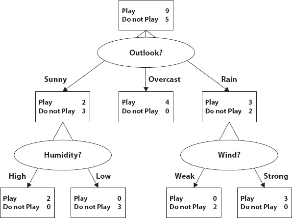
Figure 9.1 Decision tree example.
9.5 Decision Tree Algorithms
Among the various selection tree measurements, J ID3 and C4.5. R. Quinlan, are the two commonly used. A further computation is Breiman’s CART. A brief description of each of these is given below.
9.5.1 ID3 Algorithm
Ross Quinlan created recursive Dichotomiser 3 in 1986. It’s sometimes termed approximation ID3. It’s represented by the previous estimate. ID3 relies on Hunt’s estimation. It’s a simple tree learning estimate. The iterative inductive approach uses ID3 to segment images. The whole thinking in ID3 calculation creation is developed via the top-down inquiry of unique sets to look at the output from each hub in the tree [13, 14]. A calculation, Data benefit, may be the most important factor with the end goal of trait choice. Trait determination is an essential component of grouping sets. Data gathering encourages the portion of the investigations’ importance. This needs to take into account reducing observations needed to define a learning collection. ID3’s choice on the division character trait is related to data gain way of measuring. Claude Shannon concocted estimating data gain by entropy in 1948.
ID3’s tendency to the trees developed. If formed, the tree should be smaller, and the place characteristics with lower entropies should be near the tree head. In building tree models, ID3 recognizes all land. It’s the key loop ID3 acknowledges. Calculation ID3 update tree consecutively. Even then, the existence of ID3 disturbance doesn’t even provide an accurate result. Therefore, ID3 wants to deliver comprehensive data preparation before its use in the tree structural model. These trees are usually used for various purposes. Figure 9.2 shows the essential usage strategy of ID3 calculation as introduced.

Figure 9.2 Shows the ID3 algorithm.
ID3 computation problems exist. The resulting option tree for the configuration model is one problem. This is due to the systematic separation of entity split development instead of the whole tree’s progress. The consequence of this method is selection trees that are overly accurate through the use of inconsistent or irrelevant circumstances. This outcome has consequences. This is the obstacle of categorizing cryptic models or models of scattered standard esteems. Tweaking is usually used to reduce the selection of trees. However, this approach does not work efficiently for inadequate knowledge collection requiring algorithms rather than straightforward classification [15].
Algorithm C4.5
Ross Quinlan, in 1993, modified an ID3 estimation. C4.5 ID3 redesign. C4.5 is like its predecessor, based on Hunt’s measurement, which has a linear application. Tree pruning in C4.5 is post-creation.
If developed, it passes through the tree and helps to eliminate irrelevant branches by subordinating them with leaf centers [16]. Both nonstop and all-out traits are worthy in tree model structure in C4.5, not at all like in ID3. It utilizes categorization to handle consistent qualities. This categorization is finished by making a limit and isolating the characteristics dependent on their situation regarding this edge [17, 18]. Guarantee of the perfect separating feature, as in ID3, is per Data arrangement at-tree center. In C4.5, departing feature evaluation is the methodology of increasing the amount of polluting impact. C4.5 will begin to prepare data with insufficient attributes. It sees the insufficient attributes as “?” It also deals with different cost characteristics. C4.5 simply ignores the key qualities of benefit and entropy.
CART Algorithm
Order and relapse tree calculation, otherwise called CART, is an improvement by researcher. From its name, it can create arrangements and relapse model trees—truck parallel objects in definition trees arrangement. Like ID3 and C4.5, it focuses on Hunt’s projections and can run sequentially.
Small analogy and continuous attributes are indeed sufficient in CART option tree construction. That’s like C4.5 to work with lacking attributes in Results. The truck uses the Gini recording dividing test to assess the splitting product for tree construction of choice. It provides coupled parts parallel selection trees of its use of the double division of features. This seems to be special in ID3, and C4.5 split formation. Gini Index test, unlike ID3 and C4.5 estimates, does not use probabilistic suspicions. Finicky divisions are therefore replanted following expense intricacy. This increases tree accuracy.
9.5.2 Separate and Conquer Algorithm
Independent and -Conquer calculations, for example, AQ community, CN2, Rules Extractor-1 and RULES category of measurements whereby guidelines are prompted by a set of features.
RULES Implementation Family
The following is a succinct representation of all application community iterations.
RULES-1
Pham and Aksoy [19] developed RULES-1 (Rule Extraction System-1) [20]. RULES-1 execution tends to focus on entity rules incomparable class configurations—object has its attributes and characteristics, making them human. For example, if an object has Na as the number of attributes, then the norm can fall between one and Na standards. In a paper set, the whole of their qualities and benefits create a display. The shoe size is equivalent to all outnumbers, all being equivalent. Possibly there will be Na focus on traditional reporting.
In the corresponding framework, the system looks at each component to check whether that element as the situation can be appropriate for a norm. If any part in that circle applies to a solitary class, it may help structure a norm. Although it refers to more than one class, the primary indicators aspect is overlooked. When RULES-1 tests all parts, it re-evaluates all models against the up-and-comer rule to ensure all is set. Off chance that some models remain classified information, another cluster is formed with all unclassified models, and the following technique focus is initiated. If no more unclassified models, the research is finished. This continues before one or more cycles are correctly ordered Na. This period can be found below in Figure 9.3.

Figure 9.3 Shows RULES flow chart.
RULES-1’s favorable conditions and limitations. A big advantageous position is that the problem of conditions is not superfluous due to the insignificant condition checking point. There’s no remote management necessity provided that the Cpu doesn’t have to track all models in the memory all the time. Nonetheless, the system has problems with disproportionately large amounts of rules chosen, as RULES-1 has no solution to sifting through sizes. Additionally, it has a long planning time linked to it when dealing with a problem with an enormous number of characteristics and attributes. A further flaw in RULES-1 that it cannot interact with computational attributes or faulty designs [21, 22].
RULES-2
After RUL1ES-1, Pham and Aksoy imagined RULES-2 in 1995. RULES-2 is similar to RULES-1 about how it defines rules; however, the key difference is that RULES-2 considers the approximation of one unclassified guide to establishing a norm for organizing that design as applied to the estimate of all unclassified models in each circle. Correspondingly, RULES-2 works better. It also gives the client some control over what series of regulations to extricate. A further favored role is the ability of RULES-2 to engage with unfinished designs and to deal with numerical and ostensible qualities when screening through non-significant systems and automatically away from redundant circumstances [23].

Figure 9.4 RULES-3 calculation.
RULES-3
RULES-3 had been the effective development, building on the advantages of the preceding structures and implementing new highlights, for example, more simplified rule sets and methods to adjust how consistent the concepts outlined should be. RULES-3 clients can define the base set of responsibilities to create a norm. It is of interest—the criteria will be more precise, and not the same amount of activities based would be required to find the correct recommendation [24]. This cycle can be summed up as underneath in Figure 9.4 [25].
RULES3-Plus
In 1997 Pham and Dimov based upon RULES-3’s capacity to shape rules in their production of RULES-3 PLUS calculation [26].
RULES-3 Plus is much more capable of looking at rules and regulations than RULES-3, applies the pillar search procedure rather than greedy exploration, and uses the so-called H metric to help select rules as to how appropriate and specific they are.
Nevertheless, RULES-3 Plus has its drawbacks—its efficiency is not an inevitable outcome, as it will usually train extensively to cover all info. Also, the H calculation is an incredibly disturbing measurement and does not achieve the most precise and specific results. Even though RULES-3 Plus discrete its enduring valued traits, its technique of discretion does not adhere to any fixed principles; it is self-assertive and does not attempt to discover any details in the Data, which hinders RULES-3 Plus’ ability to learn new guidelines. The RULES-3 Plus standard framing scheme is illustrated in Figure 9.5 [27].
RULES-4
RULES-4 [28] offered the opportunity to progressively disassociate links in the RULES family by treating design in effect. From 1997, Pham and Dimov developed RULES-4 as the key gradual learning measurement in the RULES family. They developed it as a minor departure from RULES3 Plus, and it has some extra points of interest—particularly the ability to store models in short-term memory (STM) when they become accessible and ready. Another advantageous position of RULES-4 is the right of the customer to specify the scale of the STM supplying used to make specifications.
Once that database is complete, RULES-4 may draw new concepts on RULES-3 Plus’ info. Pham and Dimov explain the incremental estimate 6.
STM consistently vacant, and it’s initialized with a lot of analyzed models. LTM contained the recently removed guidelines or underlying principles characterized by the user. Figure 9.6 illustrates the RULE-4 incremental induction procedure.

Figure 9.5 Procedure of RULE-3 plus rule forming.
RULES-5
Pham developed RULES-5 from 2003, centered on RULES-3 Plus upsides. They tried to overcome some RULES-3 Plus shortcomings in their recently developed approximation titled RULES-5. It implements a policy to manage infinite attributes, so there is no quantification criterion [29]. The primary step in RULES-5 computation is to pick the state, and the technique for dealing with feature progresses. The developers explain this center measure as observes: RuleS-5 ‘s rule abstraction loop considers only the conditions apart from the nearest model (CE) secured by the extricated Rule and has no position with the analytical class. Any data processing can integrate both income and discrete qualities. A test is used to record the distinction between any two types in the knowledge set, whether it integrates distinct qualities or continues with those.

Figure 9.6 RULE-4 incremental induction procedure.
The key benefit of understanding RULES-5 from past RULES calculations is its ability to generate very accurately fewer laws. This needs some effort and time [30].
RULES-6
RULES-6 originally developed by Pham and Afify in 2005, using RULES-3 Plus as a basis. RULES-6 is a fast method of discovering IF-THEN concepts from given models; it is also more straightforward in determining rules and how it manages emerging middle. Since Pham and Afify created RULES-6 to extend and enhance RULES-3 Plus by adding the ability to manage disturbance in the dataset, RULES-6 is both more reliable and user-friendly and does not suffer similar log jams throughout the learning cycle as it is not hampered by needless subtleties. Making it significantly more efficient, RULES-6 uses more straightforward measures for qualifying rules and checking endless quality in measurements, which encouraged more improvement in calculation shows. Figure 9.7 represents the RULES-6 pseudo-code. The Induce One Rule technique completes a specific general search [31].
RULES3-EXT
Author [32] developed another inductive learning calculation called RULES3-EXT in 2010. Various real disservices exist in RULES-3 to resolve them effectively. The conceivable theory outcomes of RULES3-EXT are as follows: it is ideal for removing unnecessary models, enabling customers to make adjustments as needed in the form of a feature request, if any of the extricated rules cannot be sufficient certainty by an unmistakable model, the system can deal with slightly fire rules and can deal with less planned records to extricate a repository of two records. The key steps showing the RULES3-EXT deployment cycle are given below in Figure 9.8 [33].
RULES-7
The RULES class extended to Rules-7 [34] or RULe Extraction System Version 7, which improves its precedent RULES-6 by correcting a portion of its drawbacks. RULES7 uses a general specific data-gathering panel review to decide the best guideline. It selects a seed model progressively transferred by the Induce Rules method to the Induce One Rule method after calculating MS, which is the base number of cases to be protected by ParentRule. Two very different ParentRuleSet and ChildRuleSet are initialized to Empty.

Figure 9.7 Pseudocode portrayal of RULES-6.

Figure 9.8 RULES3-EXT calculation.
The program called SETAV makes a precedent norm signifying all circumstances in the norm counterpart as non-existent. BestRule (BR) is the broadest concept generated by the SETAV methodology, and the ParentRuleSet is recognized for specialization. The loop constantly repeats until the ChildRuleSet is unclaimed, and there are no more values to replicate into ParentRuleSet. The RULES-7 estimation only recognizes certain criteria in the ParentRuleSet that contain more than MS. When the Rule is met, the standard adds a new “Legitimate” requirement by simply modifying the “exist” requirement banner from its original “no” to “yes” [35]. This form, called ChilRule (CR), will be tested for rule replication to assure ChildRuleSet is released from any replication. RULES-7 used an identifiable control system to correct a few flaws in RULES-6. Since the copy rule look at has just been conveyed, the calculation does not need to make more progress towards the conclusion to remove ChildRuleSet copy rules that help rescue massive time when compared to RULES-6 [36]. Figure 9.9 displays a RULES-7 process flow.
RULES-8
In 2012, Pham [3] developed another standard acceptance calculation called RULES-8 to interact with discrete and continuous factors without any pre-preparation need. It can also handle noisy data in data collection. RULES8 was suggested to fix its precursors’ inconsistencies by selecting an up-and-comer opportunity rather than a seed guideline to define another level. It selects the user credit an opportunity to ensure the best recommendation is the created law. Choosing conditions depends on applying an explicit heuristic H test. The arrangement of parameters is rendered by continuously applying H-dependent conditions. This test surveys each recently formulated guideline’s data content. There is also an enhanced disassociation approach applied to rules to provide more simplified utilizes the idea and decrease coverage between rules.

Figure 9.9 A disentangled depiction of RULES-7.
The sample feature value is called a requirement that is fitted to cover most models when applied to a norm. RULES-8 calculation, specific in comparison to its predecessors in the RULES family, initially selects a seed trait interest and then uses a specialization loop to locate an overall guideline by slowly adding new conditions. Figure 9.10 demonstrates RuLES-8 ‘s normal forming techniques [37, 38].

Figure 9.10 REX-1 algorithm.
9.5.3 RULE EXTRACTOR-1
REX-1 (Rule Extractor-1) was rendered to obtain IF-THEN from either of the models. It is an innovative estimate for inductive learning and forgives the traps faced in RULES family measurements. Entropy confidence is used to give more motivation to major characteristics. REX-1 ‘s rule enrolment period is as follows: REX-1 ascertains critical probability esteems and readjusted entropy esteems, at which point the assigns in hiking application are first set to deal with the lowest entropy esteem. Figure 9.11 displays the REX-1 formula below [39].
9.5.4 Inductive Learning Applications
Inductive learning calculations are space free and can be utilized in any errand, including characterization or example acknowledgment. Some of them are summed up below [40].
9.5.4.1 Education
Analysis of Data mining for use in learning is on the rise. This new software area, Educational Data Mining (EDM). Developing methods to identify and focus data from instructive environments is EDM’s fundamental concern. EDM may use Choice Trees, Neural Networks, Naïve Bayes, K-Nearest Neighbors, and various strategies. Through using this technique, different types of data are revealed, such as characterizations, association rules, and sorting. Recovered data can be used to establish different standards. For example, it appears to be used to forecast understudy enrolment in a particular course, expose anomalous qualities in the slips of the understudy performance, and decide the most suitable course for the understudies based on their past qualities and abilities. They may also help guide the learners on additional courses to benefit their show.
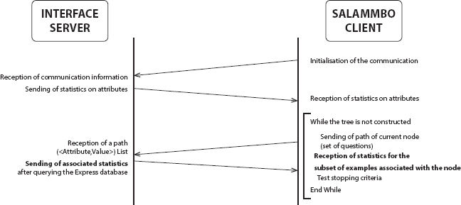
Figure 9.11 Construction procedure of fuzzy decision tree.
There are several choice tree creation measurements that are commonly used in all AI viewpoints practices, particularly in EDM. Occurrences commonly used in EDM are ID3, C4.5, Ride, CHAID, QUEST, GUIDE, CRUISE, CTREE, and ASSISTANT. J. Ross Quinlan’s ID3 and substitute, C4.5, are among the most commonly used AI tree calculations C4.5 and ID3 are similar in their behavior, but C4.5 has better methods as compared to ID3.ID3 calculation bases, deciding the best data gain, and entropy concept. C4.5 manages unreliable data. This comes at the cost of a high classification blunder rate. The forklift is another notable calculation splitting the data into two subsets adaptively. This makes the information more precise in one sub-set than in the other sub-set. The wagon will restart until a stopping state or until the uniformity norm is attained.
9.5.4.2 Making Credit Decisions
Advance organizations regularly use polls to gather data about credit candidates to decide their credit qualifications. This cycle used to be manual yet has been computerized somewhat. For instance, American Express UK utilized a measurable choice system dependent on a separate investigation to dismiss candidates under a particular edge while tolerating those surpassing another. The staying fell into a “fringe” district and was changed to credit officials for additional consideration. Notwithstanding, advance officials were exact in anticipating expected default by marginal candidates close to half of the time.
These discoveries propelled American Express UK to attempt strategies, for example, AI, to improve dynamic measures. Michie and his partners utilized an enlistment strategy to create a choice tree that made exact expectations of about 70% of the marginal candidates. It doesn’t just improve the precision however it causes the organization to give clarifications to the candidates.
9.5.5 Multidimensional Databases and OLAP
The social model of Data gives proficient instruments to store and manage the huge measure of Data at an individual level. The OLAP wording has been proposed for the sort of advances giving intends to gather, store, and manage multidimensional Data, with the end goal of conveying investigation measures. In the OLAP system, Data are put away in Data hypercubes (basically called solid shapes). A block is a lot of Data composed as a multidimensional cluster of qualities speaking to measures more than a few measurements. Pecking orders might be de ned on measurements to compose Data on more than one degree of collection.
A 3D shape B is assigned by methods form measurements, each measurement related with a space Di of qualities, and by a lot of components SB(d1; :::; dm)(with di ∈ Di; i= 1; :::; m) having a place with a set V of qualities. Mathematical activities have been characterized on hyper shapes to picture and examine them: move up, drill down, cut, dice, pivot, switch, part home, push furthermore, more traditional activities, for example, join, association, and so forth.
The union is utilized to accelerate inquiries. It comprises precomputing all or part of the shape with a conglomeration work. A portion of the most costly calculations are made before the question, and their outcome is put away in the Database to be utilized when required.
9.5.6 Fuzzy Choice Trees
Choice trees are notable apparatuses to speak to Data, and a few inductive learning techniques exist to develop a choice tree from a preparation set of Data. The utilization of the Fuzzy set hypothesis upgrades the understandability of choice trees while thinking about mathematical qualities. Besides, it empowers to consider uncertain qualities. Choice trees can be summed up into Fuzzy choice trees while thinking about Fuzzy qualities as marks of edges of the tree. Along these lines, traditional strategies have been adjusted to deal with Fuzzy qualities either during their development or while characterizing new cases.
Let A = {A1; :::; AN} be a lot of qualities and let C = {c1; :::; cK} be a lot of classes. A and C empower the development of models: every model ei is formed by a portrayal (an N-tuple of trait esteem sets (Aj; vol)) related to a specific class ck from C.
Given a preparation set E = {e1; :::; en} of models, a (Fuzzy) choice tree is developed from the root to the leaves by progressive parceling of the preparation set into subsets. The development cycle can be part of three basics steps. An ascribe is chosen on account of a proportion of segregation H (stage 1) that arranges the credits as indicated by their exactness concerning the class. The parceling is finished by methods for a parting procedure P (stage 2). A halting rule T empowers us to quit parting a set and to develop a leaf in the tree (stage 3). To assemble Fuzzy choice trees, the usually utilized H measure is the star-entropy measure characterized as:

where vj1,……, vjL are values from E for characteristic Aj. This measure is acquired from the Shannon proportion of entropy by presenting Zadeh’s likelihood measure P* of Fuzzy occasions.
The calculation to develop Fuzzy choice trees is actualized in the Salammb framework. The yield of the framework is a Fuzzy choice tree that can be considered as a lot of found grouping rules.
9.5.7 Fuzzy Choice Tree Development From a Multidimensional Database
The multidimensional data set administration framework may either send just essential data on Data, or figure complex Fuzzy tasks and accumulations, or any of the middle arrangements.
In the primary case, the coordination of other inductive learning applications will be simpler. They in reality, all require at most reduced level straightforward total calculation, for example, check (for example, frequentist calculations). So the traded essential measurements we propose will even now be required. The various more unpredictable calculations will stay outside of the multidimensional Database administration framework, which will in this way be conventional. Then again, the subsequent arrangement upgrades the totals’ calculations (for example, calculation of complex capacities as, for example, entropy proportion of a set) since multidimensional Database administration frameworks are intended for this sort of task.
In our framework, an interface is executed that comprises in trading, for every hub of the tree, measurements on the Data related to the current hub. These Data may either be singleton esteems or spans, which empower us to develop Fuzzy choice trees. These insights are figured utilizing OLAP questions to extricate a sub-shape from the Database and bringing measurements on it with accumulation capacities. As nitty-gritty beforehand satisfy, they either concern fundamental rely on the cells in the extricated Data 3D shape or may require more mind-boggling analytics, for example, entropy calculation. These insights are then utilized by Salammb to pick the best credit to proceed in the development of the tree. At that point, stage 1 of the choice tree development measure is supplanted by the accompanying cycle:
Step 1: Salammb sends an inquiry indicating the current hub to create in the tree. This inquiry is made by a set out of inquiries on estimations of properties that make the way from the root to this hub.
Step 2: The interface program inquiries the Data 3D shape and returns for each trait esteem, for each class esteem, the relating measurements registered from occurrences of the data set that satisfy the Salammb’s question.
Step 3: Salammb gets the measurements and picks the best traits. Contingent upon the arrangement traded measurements are either frequentist tally of occasions or separation proportion of each trait.
9.5.8 Execution and Results
This framework has been created through customer/worker engineering, including a multidimensional Database administration framework (Oracle Express) on SunOS, an Oracle social data set worker on a PC under Microsoft Windows NT, a C++ interface on Windows NT, and Salammb running on a second SunOS station (Figure 9.12).
This proposed framework was assessed on Data from a Data distribution center of the French Educational Department, containing singular outcomes in secondary school declaration through two years (around 1,000,000 records). Examples of found guidelines are:

Figure 9.12 Offered multidimensional databases architecture from fuzzy data mining technique.
R1: If the secondary school is open, and the endorsement class is financial aspects, at that point, the extent of up-and-comers that prevail with notice (rather great, great, or awesome) is little.
R2: If the secondary school is private, and the scholastic year is 1996, and the strength of the understudy is unknown dialect 2, and the certificate is STI”, at that point the extent of applicants that prevail with notice (rather great, great, or awesome) is enormous.
9.6 Conclusion and Future Work
In this paper, another methodology is introduced to fabricate Fuzzy choice trees from a Data distribution center utilizing the OLAP innovation. This methodology prompts the meaning of a customer/worker engineering that relates the Salammb programming, a Fuzzy choice tree development framework, with Oracle Express, a multidimensional DBMS.
Designers also focused on how inductive learning encourages the system to interpret validity and reliability and instances in past data or data planning and emphasize necessary to characterize. This paper presented a description of inductive learning concepts as brief depictions of current calculations. Numerous characterization calculations were discussed in writing but, due to ease of usage, the options tree is the most widely used instrument, just as simple as other order calculations. Option tree calculations for ID3, C4.5, and CART were explained individually. Experts attempted to boost coverage estimates to overcome the effects of distance and -vanquish projects. Induce regulates genuinely from the database itself is preferable as opposed to collecting them from an option tree. The calculation of the RULES group is used to trigger several order rules from a range of styles for objects with one defined class.
Results are promising and urge us to start further research, among which the tests with different Databases, further examinations between the various arrangements we have introduced here to trade measurements, the incorporation of other learning techniques, the execution of an all the more well-disposed UI, and the treatment of Fuzzy Data (loose and additionally unsure) in the hypercubes.
References
1. Elgibreen, H.A. and Aksoy, M.S., RULES-TL : A Simple and Improved Rules. J. Theor. Appl. Inf. Technol., 47, 1, 28–40, 2013.
2. Mohamed, A.H. and Bin Jahabar, M.H.S., Implementation and Comparison of Inductive Learning Algorithms on Timetabling. Int. J. Inf. Technol., 12, 7, 97–113, 2006.
3. Trnka, A., Classification and Regression Trees as a Part of Data Mining in Six Sigma Methodology. Proc. World Congr. Eng. Comput. Sci., vol. I, 2010.
4. Tolun, M.R. and Abu-Sound, S.M., An Inductive Learning Algorithm for Production Rule Discovery, pp. 1–19, Department of Computer Engineering Middle East Technical University, Ankara, Turkey, 2007.
5. Deogun, J.S., Raghavan, V.V., Sarkar, A., Sever, H., Data Mining : Research Trends, Challenges, and Applications, in: Roughs Sets and Data Mining: Analysis of Imprecise Data, pp. 9–45, Kluwer Academic Publishers, USA, 1997.
6. Khan, R. and Raja, R., Introducing L1—Sparse Representation Classification for facial expression. Imp. J. Interdiscip. Res. (IJIR), 2, 4, 115–122, 2016.
7. Witten, I.H. and Frank, E., Data Mining: Practical Machine Learning Tools and Techniques, 2nd edition, Morgan Kaufmann, Burlington, Massachusetts, 2005.
8. Bahety, A., Extension and Evaluation of ID3—Decision Tree Algorithm, pp. 1–8, University of Maryland, College Park, 2009.
9. Stahl, F., Bramer, M., Adda, M., PMCRI : A Parallel Modular Classification Rule Induction Framework, in: Machine Learning and Data Mining in Pattern Recognition, pp. 148–162, Springer, Berlin, Heidelberg, 2009.
10. Kurgan, L.A., Cios, K.J., Dick, S., Highly scalable and robust rule learner: Performance evaluation and comparison. IEEE Trans. Syst. Man Cybern. B. Cybern., 36, 1, 32–53, Feb. 2006.
11. Codd, E.F., Codd, S.B., Salley, C.T., Providing OLAP (On-Line Analytical Processing) to User-Analysts: An IT Mandate, Hyperion Solutions Corp, Sunnyvale, CA, 1993.
12. Mitchell, T.M., Decision Tree Learning, in: Machine Learning, pp. 52–80, McGraw-Hill, Singapore, 1997.
13. Baradwaj, B.K. and Saurabh, P., Mining Educational Data to Analyze Students’ Performance. Int. J. Adv. Comput. Sci. Appl., 2, 6, 63–69, 2011.
14. Rathee, A. and Prakash Mathur, R., Survey on Decision Tree Classification algorithms for the Evaluation of Student Performance. Int. J. Comput. Technol., 4, 2, 244–247, 2013.
15. Pathak, S., Raja, R., Sharma, V., Ambala, S., ICT Utilization and Improving Student Performance in Higher Education. Int. J. Recent Technol. Eng. (IJRTE), 8, 2, 5120–5124, July 2019.
16. Verma, T., Raj, S., Khan, M.A., Modi, P., Literacy Rate Analysis. Int. J. Sci. Eng. Res., 3, 7, 1–4, 2012.
17. Yadav, S.K. and Pal, S., Data Mining: A Prediction for Performance Improvement of Engineering Students using Classification. World Comput. Sci. Inf. Technol. J., 2, 2, 51–56, 2012.
18. Wu, X., Kumar, V., Quinlan, J.R., Ghosh, J., Yang, Q., Motoda, H., McLachlan, G.J., Ng, A., Liu, B., Yu, P.S., Zhou, Z.-H., Steinbach, M., Hand, D.J., Steinberg, D., Top 10 algorithms in data mining. Knowl. Inf. Syst., Springer, 14, 1, 1–37, Dec. 2007.
19. Pham, D.T. and Aksoy, M.S., RULES: A simple rule extraction system. Expert Syst. Appl., 8, 1, 59–65, Jan. 1995.
20. Aksoy, M.S., A Review of RULES Family of Algorithms. Math. Comput. Appl., 13, 1, 51–60, 2008.
21. Pham, D.T. and Dimov, S.S., An Efficient Algorithm For Automatic Knowledge Acquisition. Pattern Recognit., 30, 7, 1137–1143, 1997.
22. Pham, D.T. and Dimov, S.S., An algorithm for incremental inductive learning. Proc. Inst. Mech. Eng. Part B J. Eng. Manuf., 211, 3, 239–249, Jan. 1997.
23. Pham, D.T., Bigot, S., Dimov, S.S., RULES-5: A rule induction algorithm for classification problems involving continuous attributes. Proc. Inst. Mech. Eng. Part C J. Mech. Eng. Sci., 217, 12, 1273–1286, Jan. 2003.
24. Pham, D.T. and Afify, A.A., RULES-6: A simple rule induction algorithm for supporting decision making. 31st Annu. Conf. IEEE Ind. Electron. Soc. 2005. IECON 2005, p. 6, 2005.
25. Mathkour, H.I., RULES3-EXT Improvements on RULES-3 Induction Algorithm. Math. Comput. Appl., 15, 3, 318–324, 2010.
26. Shehzad, K., EDISC: A Class-Tailored Discretization Technique for Rule-Based Classification. IEEE Trans. Knowl. Data Eng., 24, 8, 1435–1447, Aug. 2012.
27. Pham, D.T., A Novel Rule Induction Algorithm with Improved Handling of Continuous Valued Attributes, Cardiff University, UK, 2012.
28. Akgöbek, Ö., Aydin, Y.S., Öztemel, E., Aksoy, M.S., A new algorithm for automatic knowledge acquisition in inductive learning. Knowledge-Based Syst., 19, 6, 388–395, Oct. 2006.
29. Aksoy, M.S., Almudimigh, A., Torkul, O., Cedimoglu, I.H., Applications of Inductive Learning to Automated Visual Inspection. Int. J. Comput. Appl., 60, 14, 14–18, 2012.
30. Rajadhyax, N. and Shirwaikar, R., Data Mining on Educational Domain, pp. 1–6, ArXiv, India, 2010.
31. Alhammadi, D.A. and Aksoy, M.S., Data Mining in Education—An Experimental Study. Int. J. Comput. Appl., 62, 15, 31–34, 2013.
32. Quinlan, R., C4. 5 : Programs for Machine Learning, vol. 240, pp. 235–240, Kluwer Academic Publishers, Kluwer Academic Publishers, Boston. Manufactured in The Netherlands, 1994.
33. Langley, P. and Simon, H.A., Applications of Machine Learning and Rule Induction, ACM Digital Library, Palo Alto, CA, 1995.
34. Pathak, S., Raja, R., Sharma, V., Ramya Laxmi, K., A Framework Of ICT Implementation On Higher Educational Institution With Data Mining Approach. Eur. J. Eng. Res. Sci., 4, 5, 2019.
35. Pathak, S., Raja, R., Sharma, V., The Impact of ICT in Higher Education. IJRECE, 7, 1, 1650–1656, January–March, 2019.
36. Agrawal, G.A. and Sarawagi, S., Modeling Multidimensional Databases, in: Proc. of the 13th Int. Conf. on Data Engineering, Birmingham, U.K., 1997.
37. Bouchon-Meunier, B., Marsala, C., Ramdani, M., Learning from Imperfect Data, chap. 8, in: Fuzzy Information Engineering: A Guided Tour of Applications, D. Dubois, H. Prade, R.R. Yager (Eds.), pp. 139–148, John Wiley and Sons pub., Hoboken, New Jersey, USA, 1997.
38. Bouchon-Meunier, B. and Marsala, C., Learning Fuzzy Decision Rules, chap. 4, in: Fuzzy Sets in Approximate Reasoning and Information Systems, J. Bezdek, D. Dubois, H. Prade (Eds.), pp. 279–304, Kluwer Academic Pub., Handbooks on Fuzzy Sets Series, Dordrecht, Netherlands, New York, NY, Norwell, MA, London, UK, 1999.
39. Chen, M.S., Han, J., Yu, P.S., Data Mining: An Overview from a Database Perspective. IEEE Trans. Knowl. Data Eng., 8, 6, 866–883, 1996.
40. Harinarayan, V., Rajaraman, A., Ullman, J., Implementing data cubes efficiently, in: Proc. of the 1996 ACM SIGMOD Int. Conf. on Management of Data, pp. 205–216, 1996.
41. Marsala, C., Bouchon-Meunier, B., Ramer, A., Hierarchical Model for Discrimination Measures, in: Proceedings of the IFSA’99 World Congress, Taipei, Taiwan, August 1999, pp. 339–343.
- *Corresponding author: [email protected]