2

Data Structures, Types, and Formats

This chapter is all about data storage. Occasionally, a data analyst will have to collect their own data, but for many, the company already has data stored and ready for use. During their career, a data analyst may encounter data stored in several different formats, and each format requires a different approach. While there are hundreds, if not thousands, of different formats, the exam only covers the most common, and this chapter will go over what you need to know about them.

Here, we will discuss things such as how data is actually stored in a database, which includes whether or not it is structured, deciding what kind of data is stored in it, and whether the database is organized to follow a specific data schema to make it more efficient. We will also cover common database archetypes, or data storage solutions that are arranged in a specific way for a specific purpose, such as a data warehouse or a data lake. After that, we will discuss why updating data that is already stored can be problematic and a few approaches you can take depending on your goals. Finally, we will wrap up this chapter by discussing data formats so that you can tell what kind of data to expect from each format.

In this chapter, we’re going to cover the following main topics:

• Understanding structured and unstructured data
• Going through a data schema and its types
• Understanding the concept of warehouses and lakes
• Updating stored data
• Going through data types and file types

Understanding structured and unstructured data

More often than not, data is stored in a database. Databases are simple places where data can be electronically stored and accessed. They can be stored on a single computer, a cluster, or even in the cloud. Databases come in every shape and size, but all of them fall into one of two categories:

• Structured
• Unstructured

Structured databases

If a database is structured, it follows a standardized format that allows you to set rules as to what kind of data can be expected and where. That is to say that there is, hopefully, a clear and logical structure to how the data is organized. There are two main database archetypes that the exam considers structured:

• Defined rows/columns
• Key-value pairs

Defined rows and columns refer to tables or spreadsheets. This is the format that most people are familiar with and is, by far, the most common in the field of data analytics. Usually, every column in the grid represents a variable or type of data collected, and every row represents a single entry or data point. The following screenshot shows a simple table that counts beans:

Figure 2.1 – Structured database: defined rows and columns

In the preceding screenshot, the columns are vertical and represent the different variables, while the rows are horizontal and represent a different entry or data point. The cells are specific values or counts that make up a data point.

Key-value pairs store each data point as a data object; every object in a series has the same set of keys, but the values for them can be different. In the following code snippet, each key represents a variable, and each value is the data collected for it, while each object is a data point:

"Beans" : [
     {
          "Total" : 10,
          "Red" : 3,
          "Blue" : 4,
          "Yellow" : 3
     },
     {
          "Total" : 12,
          "Red" : 2,
          "Blue" : 6,
          "Yellow" : 4
     },
     {
          "Total" : 11,
          "Red" : 3,
          "Blue" : 5,
          "Yellow" : 3
     }
]

This is the same information as shown in Figure 2.1, but now it is stored with each row being a data object defined by {}. The column names ("Total", "Red", "Blue", and "Yellow") are the keys. The keys are unique in that they cannot be repeated within a data object. For example, you cannot have two keys named "Yellow". However, all objects within a set usually have the same keys. The numbers represent the values or are the same as individual cells within a table.

Unstructured databases

Unstructured data has, more or less, no attempt at organization. You can think of these as big buckets of data, often in the form of a folder, where individual files or random data objects can be dropped. The exam breaks these down into two groups:

• Undefined fields
• Machine data

In this case, an undefined field is sort of a catch-all for file types that do not fit into a structured database nicely. These include several different file types, such as the following:

• Text files
• Audio files
• Video files
• Images
• Social media data
• Emails

These are all data types that, by default, store every data point as a separate file, which makes it difficult to keep them in a conventional structured database.

The other type of unstructured data recognized by the exam is machine data. When data is automatically generated by software without human intervention, it is often considered machine data. This includes automated logging programs used by websites, servers, and other applications, but it also includes sensor data. If a smart refrigerator logs measurements of temperature and electricity used at a regular time interval, this is considered to be machine data.

Relational and non-relational databases

Another way to categorize databases is whether they are relational or non-relational. Relational databases store information and how it relates to other pieces of information, while non-relational databases only store information.

This gets a little confusing when we look at query languages for pulling information out of databases. The majority of query languages are variations of Structured Query Language (SQL). Anything that isn’t based on SQL is considered NoSQL. Now, in common usage, everything that uses SQL is structured and relational, and everything that is NoSQL is unstructured and non-relational. However, this is not quite true. This can get a little confusing, so we will break it down into the following four main points:

• All SQL databases are structured and relational
• All non-relational databases are unstructured
• Some NoSQL databases are structured and relational
• Some NoSQL databases are unstructured, but still relational

Let’s start from the top. All SQL databases are structured and relational. SQL databases are broken down into tables. Tables are inherently structured and show how one point connects to another, so they are relational. For example, if you look at a table, you know how every cell in a column is related (they are all different data points that record the same measurement or classification) and how every cell in a row is related (they are all different measurements of the same data point).

All non-relational databases are unstructured. This means that all databases that do not show how things are related inherently have no structure. Any structural organization would show relationships. For example, if you have a database that is nothing but a folder for audio files, there is nothing that shows the relationships between the files. Each audio file is its own discrete unit, and there is no structure between them.

Some NoSQL databases are structured and relational. Just because something is not based on SQL does not mean that it has no structure. For example, the exam considers key-value pairs to be structured and relational, but these are most often used in JSON files, which are considered NoSQL.

Some NoSQL databases are unstructured, but still relational. There exist databases called graph databases. These are NoSQL databases, where the nodes are stored separately in an unstructured manner, but they also store the relationships between every node. If a database stores the relationships between each node, it is relational.

This seems a little jumbled, but the most important things to remember are that tables and key-value pairs are structured and relational, while undefined fields and machine data are unstructured and, unless otherwise stated, non-relational. This can be summarized in Figure 2.2:

Figure 2.2 – Structure and relationships

Now, whether something is relational or structured is not the only consideration you need to think about when you are storing data in a database. How the tables themselves are arranged makes a huge difference in how useful and efficient a database is, so it’s time to learn about schemas.

Going through a data schema and its types

An SQL database—structured and relational—is often made up of more than one table. In fact, more complicated databases may have dozens or even hundreds of tables. Every table should have a key. A key is a variable that is shared with another table so that the tables can be joined together. We will discuss specifics on joins later in this book. In this way, all the tables can be connected to one another, even if it would take several joins to do it. As you can imagine, these databases can be confusing, inefficient, and impractical. To make databases cleaner and easier to use, how tables are organized and interact with each other often follows a few common patterns. These patterns are called data schemas. There are several different popular schemas, and each meets specific needs, but this exam only covers two of the most basic schemas:

• Star
• Snowflake

The schemas are named after the shapes the tables make when you graph out how they are related.

Star schema

A star schema is one of the simplest schemas. At the center is a key table (sometimes called a fact table) that holds metrics, but they also have key variables for every other table in the database. Around the key tables, there are tables called dimension tables. Each dimension table has one key variable to connect to the key table and several other variables for storing information. Because all the dimension tables are connected directly to the central key table, the shape looks like a star. In Figure 2.3, you can see an example of the basic database of this schema, with the key table in the center and the dimension tables attached:

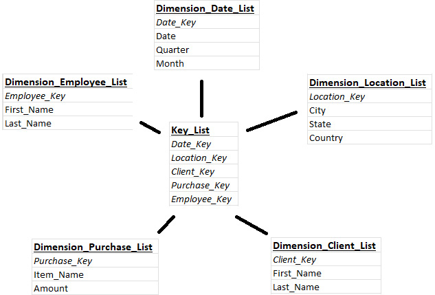
Figure 2.3 – Star schema

As you can imagine, there are pros and cons to this type of schema.

Pros:

• Simple (there are generally fewer tables)
• Fewer joins are required
• Easier to understand how the tables relate to one another

Cons:

• High redundancy (a lot of data is repeated)
• Denormalized (because of the high redundancy)

This schema is more user-friendly, but not the most efficient for larger databases. In Figure 2.4, you will see a diagram detailing a join with a star schema:

Figure 2.4 – Joining with a star schema

Imagine you wanted information from Dimension_Date_List and Dimension_Client_List together. You only need to join Dimension_Date_List to Key_List and then Key_List to Dimension_Client_List. That is only two joins, and you will never need more than two joins to connect any two tables in a star schema. That said, because the information is condensed to fit around a single table, information is often repeated, and it is not the most efficient approach. For example, in the preceding diagram, Dimension_Date_List has a date variable, but then it also has quarter and month variables in the same table. The variables are repeated because they are used for different things, but are grouped together in a table in a star schema.

Snowflake schema

A snowflake schema is similar to a star schema with one main difference: there are two levels of dimension tables. There is still a key table in the middle with dimension tables connected directly to it, but there is now a second set of dimension tables that connect to the first. This doesn’t necessarily mean that there is more data than we saw in the star schema, but the data is spread out more. Figure 2.5 is a simplified example of what a snowflake schema may look like:

Figure 2.5 – Snowflake schema

Because of the branching lines coming out from the center, it is considered to look like a snowflake. Just as with a star schema, a snowflake schema has strengths and weaknesses.

Pros:

• Low redundancy (very few, if any, metrics are repeated)
• Normalized (follows a step of rules introduced by Edgar F. Codd to optimize databases)

Cons:

• More complicated (understanding how the tables relate to one another is more difficult)
• More joins are required (joining two tables may require several intermediate joins)

These are generally more efficient than star schemas, but they are less user-friendly. Because they are more complicated, it requires a greater understanding of how this specific database is structured in order to navigate it. Figure 2.6 is an example of trying to join two random tables within a snowflake schema:

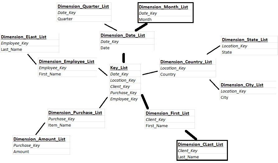
Figure 2.6 – Joining within a snowflake schema

Here, connecting any two tables may require anywhere from two to four joins. For example, if we wanted to connect Dimension_Month_List to Dimension_CLast_List, we would have to connect the Dimension_Month_List table to Dimension_Date_List, Dimension_Date_List to Key_List, Key_List to Dimension_First_List, and the Dimension_First_List table to Dimension_CLast_List. A snowflake schema only has one more level of tables than a star schema, but you can probably see how it can already be more complicated. However, the data is more spread out and does not repeat itself as much, making it more efficient. In the preceding simplified example, we see that Date has now been spread out among three tables, so there is no repeated information in any one of them.

Next, we will talk about a way to classify databases based on how they are used.

Understanding the concept of warehouses and lakes

Not all databases are used for the same purpose—they often become specialized based on how they are used. Each specialized database has a specific name, is used for different things, has different kinds of data, and is used by different people. A few of these specialized databases include:

• Data warehouses
• Data marts
• Data lakes

There are more, but these are some common types of database archetypes that you are likely to encounter. More to the point, these are the ones that will be covered in the exam.

Data warehouses

Data warehouses are most often used for structured relational tables. Usually, they hold large amounts of processed transactional data. Data warehouses are often more complicated and are used by data engineers or database administrators. Because these store large amounts of data and efficiency is more important, they are more likely to follow a snowflake schema.

Data marts

Data marts are a specialized subset of a data warehouse. They are smaller, only hold processed information on a specific topic, and have a simpler structure. Data marts usually contain customer-facing data and are considered self-service because they are designed to be simple enough for analysts or customer support employees to access by themselves. Because these databases prioritize ease of use, they often follow a star schema.

Data lakes

Data lakes store large amounts of raw, unprocessed data. They can contain structured data, unstructured data, or some combination of both. Data lakes often collect and pool data from several different sources and can include different data or file types. Because of the nature of raw information, data lakes are often used by data scientists and do not follow any specific schema.

Important note

At this stage in your career, you will not be asked to create a data warehouse or lake. These are usually made by very specialized data engineers, and many companies only have one. That said, the majority of data warehouses and lakes are created through third-party services or software. Some of the more popular approaches include Snowflake, Hevo, Amazon Web Services (AWS) data warehouse tools, Microsoft Azure data warehouse tools, and Google data warehouse tools. If you want to try practicing with these tools, I suggest you find one (I like Snowflake), and look up tutorials on that software specifically.

Enough about storing data—let’s talk about how to update data that has already been stored.

Updating stored data

Sometimes information changes, and you must update your dataset. In such cases, there are decisions that must be made. Each decision has pros and cons based on the reason you are collecting the data. For slowly changing dimensions, two cases often come up:

• Updating a current value
• Changing the number of variables being recorded

Updating a record with an up-to-date value

In most cases, you will simply add data points to the end of a table, but sometimes there is a specific value that is calculated or recorded that you need to keep as up to date as possible. Now, you have two options:

• Overwrite historical values: If you just change the value in the cell, this keeps your dataset much smaller and simpler. However, because you have lost what your value was, you no longer have access to historical data. Historical data has many uses and is required for trend analysis. If you don’t care about predicting future values of this number and just want to keep your dataset as simple as possible, this is the appropriate path.
• Keep historical values: Keeping historical values usually requires the addition of extra columns so that you can keep track of what the current value is, as well as when other values were active.

To do this, you add the following columns:

• Active Record
• Active Start
• Active End

These columns work in a direct manner. Active Record simply states whether the specified value is the most current value, and is either Yes or No. Active Start describes the date a value became active, and Active End describes the date it stopped being active. This is shown in Figure 2.7:

Figure 2.7 – Active Record

If a number is currently active, Active Record will be Yes and it will have an Active Start date, but no Active End date:

Figure 2.8 – Updated Active Record

As shown in Figure 2.8, when you are updating this value, you change Active Record to No and add an Active End date for the old value. The new value will set Active Record to Yes and receive an Active Start date. In this way, you can keep a record of all historical values. If you are more interested in being able to perform trend analyses and predict a future value using historical values than you are in keeping your dataset small and simple, this is the appropriate approach.

Changing the number of variables being recorded

Occasionally, you will need to change the number of variables being recorded, so you are adding or removing columns from a table or dataset. Whether you are adding or removing variables, you will have to decide whether or not to delete all historical data. It may seem odd, but there is a specific reason: null values, or spaces where there are no values where there should be. It doesn’t matter whether you are adding columns or removing them—either way, you will create null values.

In Figure 2.9, we are adding columns that track the color of beans, which was not tracked until the third data point. This means that all data points before you added the columns will have null values:

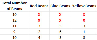
Figure 2.9 – Adding variables

In Figure 2.10, we are no longer tracking the color of the beans, so we are removing them as a variable, and normally we would just delete the columns. However, since the historical data—the first two data points—still has these columns, you will have null values for everything after you stop tracking these variables:

Figure 2.10 – Removing variables

The only way to completely avoid these null values is to dump the historical data for those columns. That said, sometimes you can’t or just don’t want to get rid of so much data, so you will have to address the null values by other means. Figure 2.11 is an example of a table that has had the null values removed:

Figure 2.11 – Deleting historical values

Okay—now you know about updated stored records. Next, we will jump into different data types and file types so that you can know what to expect from each.

Going through data types and file types

Data comes in countless formats, each requiring different treatment and capable of different things. While each programming language has its own data types, these will not be tested because the exam is vendor-neutral and does not require knowledge of any specific programming language. However, there are some generic data types that everyone working with data should know that are covered in the exam.

Data types

When discussing data types, we are talking about the format of specific variables. While there are some commonalities between programming languages, these data types may have different names or be subdivided into different groups. However, all data processing programs should have the following data types:

• Date
• Numeric
• Alphanumeric
• Currency

Date is a data type that records a point in time by year, month, and day. This data type can also include hours, minutes, and seconds. There are many different ways to format a date variable, but the International Organization for Standardization (ISO) recommends ordering your dates from the biggest unit of time to the smallest, like so:

• YYYY-MM-DD
• YYYY-MM-DD HH:MI:SS

That said, it is more important to be consistent within a dataset than to have any one particular format. When merging two datasets from different sources, check to make sure they are both using the same format for any date variables.

Numeric data is made of numbers. Different programs break this up into multiple different subtypes, but for the exam, all you need to know is that a value that is a number, no matter whether it is a decimal or a whole number, is considered numeric data.

Alphanumeric data includes numbers and letters. Just as with numeric data, these go by many different names, based on the program used, but include any value that has letters in it. The only exception is if the value is a number formatted in scientific notation.

Currency data includes monetary values. This one is pretty simple. Just remember that if the numbers show a dollar sign, it is counting money and is probably formatted as currency.

Note

The exam does not cover Boolean values or values that can only be TRUE or FALSE. Not every program recognizes Booleans as their own data type, and even if the program does, these values are often translated into a different data type for use. For example, a Boolean might be recoded as 1 and 0 instead of TRUE and FALSE, so it will be recognized and processed by a machine learning (ML) algorithm, most of which require specific data types.

Variable types

When discussing variable types in the context of this book, we are really looking at different kinds of statistical variables. What that means is if the exam indicates a specific column in a spreadsheet, you will have to be able to tell whether it is discrete, continuous, categorical, independent, or dependent. These are the types of things you will need to know when working as a data analyst to figure out whether you can run an analysis or not because every analysis has specific data requirements.

Discrete versus continuous

Discrete and continuous are two different kinds of numeric or currency data. Discrete variables are counts and usually describe whole numbers or integers. There are limited possibilities that a discrete variable can have.

Discrete examples:

• 2
• 37
• $1.23

Important note

Sometimes a number can be a decimal and still be discrete. For example, when counting currency, $1.23 can still be considered discrete, because the values after the period represent cents that can be counted individually. However, $1.235 would no longer be considered discrete because there is no way to count half of a coin.

Continuous variables are not limited to whole numbers and can represent an infinite number of values between two points. Often, these values are measured or calculated and are represented as decimals.

Continuous examples:

• 3.47
• 7.00
• $1.235

Categorical

Categorical variables, sometimes called dimensions, represent classifications or groups. Often, these are formatted as alphanumeric. There are three main types of categorical variables:

• Binary
• Nominal
• Ordinal

Binary variables are categorical variables that only have two possible states, such as TRUE and FALSE, 1 and 0, Success and Failure, or Yes and No. All Booleans are binary variables.

Nominal variables are categorical variables that contain more than two groups and have no intrinsic order. The majority of categorical variables fall into this classification. Nominal variables can include things such as color, breed, city, product, or name.

Ordinal variables are categorical variables that have an intrinsic order. These are most often represented as scales. Ordinal variables can include things such as Small, Medium, and Large or Low Priority, Medium Priority, and High Priority.

Independent versus dependent

Independence is one of the most important distinctions in statistics and will be featured heavily in the Data Analysis domain of the exam. You can consider this the purpose of a variable in a study.

Independent variables are the variables in a study that you are manipulating directly. These variables are independent because they are not influenced by anything besides you. Independent variables cause changes in other variables (or don’t).

Dependent variables are the variables in a study that you are measuring. You do not manipulate these variables at all. If these variables change, it is because of the independent variables, so the values of these variables are dependent upon the values of the independent variables.

Let’s look at an example. You run a simple study where you want to find out whetherbeing able to see impacts the accuracy of dart throwing. You gather twenty people, blindfold ten of them, have each of them throw three darts, then measure the distance those darts landed from the center of the target. In this example, the variable of sight, or whether the person was blindfolded or not, is your independent variable. You are directly manipulating this variable by choosing who to blindfold. Your dependent variable is what you are measuring. In this case, you are measuring the distance of the darts from the center of the target. After all of this is done, you will run an analysis to see whether changing your independent variable had an impact on your dependent variable.

File types

Often, data is saved on a computer as a file. Different types of data are saved as different types of files. A data analyst may be expected to deal with any number of file types, so the exam tests to see whether you can identify what kind of information can be found in the most common file types. The exam includes the following:

• Text (such as TXT)
• Image (such as JPEG)
• Audio (such as MP3)
• Video (such as MP4)
• Flat (such as CSV)
• Website (such as HTML)

Important note

While the exam is vendor-neutral and tries to avoid file types that require you to know a specific software, some of the file types are associated with a particular operating system (OS) because they are common enough that you are likely to encounter them if you are dealing with the associated data type. Also, these file types, while more common on some OSes than others, can be played on any OS. For example, a WMA file type is short for Windows Media Audio, so it is inherently associated with the Windows OS. That said, you do not need to be an expert in this OS to remember that a WMA file is an audio file.

Text

Files that only contain text may be common, depending on the specific data analytics position. Many word processing programs have their own file type. However, since the exam is vendor-neutral, we need only discuss ones that are not inherently associated with any particular program. For text files, that leaves a plain text file:

• Text (TXT)

Image

Images have several different file types that store the image in different ways. The most common include the following:

• Joint Photographic Experts Group (JPG/JPEG)
• Portable Network Graphics (PNG)
• Graphics Interchange Format (GIF)
• Bitmap (BMP)
• Raw Unprocessed Image (RAW)

Audio

Audio files include the following popular formats:

• MPEG-1 Audio Layer III (MP3)
• Waveform Audio (WAV)
• Windows Media Audio (WMA)
• Advanced Audio Coding (AAC)
• Apple Lossless Audio Codec (ALAC)

Video

Video files include the following popular formats:

• MPEG-4 Part 14 (MP4)
• Windows Media Video (WMV)
• QuickTime Video Format (MOV)
• Flash Video (FLV)
• Audio Video Interleave (AVI)

Flat

Flat files contain a simple two-dimensional dataset or spreadsheet. Again, every spreadsheet software has its own unique file type, but for the purpose of this exam, there are only two generic file types you need to know:

• Tab-Separated Values (TSV)
• Comma-Separated Values (CSV)

The difference between these two is how they separate values, or which delimiter they use.

TSV values are separated by tabs. Here’s an example:

Column1     Column2     Column3

CSV values are separated by commas. Here’s an example:

Column1,Column2,Column3

Website

When discussing website file types, we are talking about file types that can be used by a website to store or convey information to be used by a data analyst and not specifically file types used to create or manage websites. It should also be noted that these file types do represent specific languages, but you do not need to know these languages to extract information from them. For example, you do not need to understand how to structure a website with HTML to extract useful information from an HTML file; there are parsers that can do this for you. The types of website files recognized by the exam are as follows:

• Hypertext Markup Language (HTML)
• Extensible Markup Language (XML)
• JavaScript Object Notation (JSON)

HTML is a common file type that focuses on website structure, and occasionally passing information. Information is stored between tags. The tags create elements that all have specific pre-determined meanings and act in specific ways when used. Here’s an example:

<div>
     <h1>
          Store Data Here
     </h1>
<p>
          Or Here
     </p>
</div>

XML is similar to HTML, but the tags have no pre-determined meanings and don’t in a specific way. You can use whichever tags have meaning to you. For this reason, it can be difficult to parse information from an XML file that came from a new source. Here’s an example of XML:

<Dataset>
     <Data>
          Store Data Here
     </Data>
<AlsoData>
          Or Here
     </AlsoData>
</Dataset>

JSON files are not used to structure websites, unlike the other two. JSON specializes in storing and passing information. A JSON file contains a list of data objects and gives values to those objects using key-value pairs. Here’s an example:

"Dataset" : [
     {
          "Data" : "Store Data Here"
     },
     {
          "Data" : "Or Here"
     }
]

In the end, you do not need to know how to use any of these languages. Make sure you understand that while all three can pass information, JSON is the one that specializes in it. Also, know that JSON is the only one that does not contribute to website structure and is based on key-value pairs.

Summary

We covered a lot of information in this chapter. First, we covered structured and unstructured databases, and what types of data can be expected in each. Also, we talked about relational and non-relational databases, and how they relate to structured and unstructured databases. Next, we covered database schemas such as star and snowflake schemas. Then, we covered data warehouses, data marts, and data lakes. Briefly, we touched on how to update stored data. Finally, we wrapped things up with different data types and file types. This is everything you need to know about the storage of data.

In the next chapter, we will go over how this data is collected in the first place!

Practice questions and their answers

Let’s try to practice the material in this chapter with a few example questions.

Questions

1. A smart thermometer collects information about the temperature outside every 30 minutes, creates a log, and sends the data to a local database. What can you tell about the database?
   1. It is structured
   2. It is unstructured
   3. It is relational
   4. There is not enough information
2. Client-facing agents at banks are not technical experts, but require the ability to query client information. Which data schema is most appropriate for their database?
   1. Star schema
   2. Snowflake schema
   3. Galaxy schema
   4. Avalanche schema
3. You are working as a data scientist for a video-streaming website. You require access to raw, unprocessed data and video files. What is the most appropriate database style to use?
   1. Data warehouse
   2. Data mart
   3. Data lake
   4. Data mine
4. An e-commerce website has been collecting information on purchases for over a year. Now, they want more detailed geographical information to find out where their products are selling, so they start collecting information on the IP address of the person who made the purchase. This adds a new column to the dataset. What concerns might they have going forward?
   1. Historic values for the IP Address column will be null
   2. New values for the IP Address column will be null
   3. They will not know which record is active
   4. None of these
5. You are given a file with the “.png” extension at the end to process. What type of data will you find inside?
   1. Video
   2. Audio
   3. Text
   4. Image

Answers

Now, we will briefly go over the answers to the questions. If you got one wrong, make sure to review the topic in this chapter before continuing:

1. The answer is B. It is unstructured

The question tells you that the data is automatically generated and logged by a machine. This makes it machine data, and machine data is one of the two types of data that are inherently unstructured.

2. The answer is A. Star schema

A star schema is simple and focuses more on being user-friendly, making it ideal for data marts and use by less technical employees.

3. The answer is C. Data lake

A data lake is the only database style discussed that focuses on raw data. It is also the only one that can easily store structured and unstructured data or is meant for use by a data scientist.

4. The answer is A. Historic values for the IP Address column will be null

Because you are adding a new column, you will not have any values in that column from before you added it, making all historic values null by default.

5. The answer is D. Image

PNG stands for Portable Network Graphics and PNG files contain images.