CHAPTER 2
Methods of Statistical Forecasting
Instead of covering the basics of statistical modeling, this chapter aims to provide practical extensions of forecasting methods, including:
- Combining forecasts
- Handling outliers
- Forecasting in hierarchies
- Modeling extreme seasonality (items sell only during certain times of the year)
We also include a pair of articles on the growing application of data-mining techniques in forecasting, techniques that help identify variables potentially beneficial to forecasting models. Better models support management decision making, and can enhance organizational performance.
This chapter concludes with discussions of worst-case scenarios, downside risk assessment, and disruptive events, all issues given new attention after the 2008 global financial meltdown. Forecasting delivers its value by improving management decision making. A critical component of an informed decision is the proper assessment of uncertainty.
This compilation does not substitute for the many excellent books and articles about statistical modeling and other methodological aspects of business forecasting. While a “standard” text has been Forecasting: Methods and Applications (3rd Edition, 1998) by Makridakis, Wheelwright, and Hyndman, there are a number of recent offerings including the online, open-access textbook, Forecasting: Principles and Practice by Hyndman and Athanasopoulos, and Principles of Business Forecasting by Ord and Fildes. In 2014, Foresight published a compilation of Forecasting Methods Tutorials, providing useful nontechnical overviews of statistical forecasting methods.
2.1 Confessions of a Pragmatic Forecaster1
Chris Chatfield
Introduction
This paper presents some instructive highlights (and lowlights!) from a career in time-series forecasting that began in 1964. We can expect to learn from both our successes and failures, and I encourage forecasters to report both as we learn from both. I use the word pragmatic in the title to mean being sensible and practical and hope this applies to my work.
My reflections will touch on longstanding time-series methods, such as Holt-Winters exponential smoothing and Box-Jenkins, and on some newer methods based on neural networks, state-space formulations, and GARCH models. I will also discuss what is meant by a “best” forecast.
Turning to implementation issues, I will discuss the construction of prediction intervals, the handling of model uncertainty, the combining of forecasts, and the effect of differing numbers of items to be forecasted. Publication bias is of concern to me and I will also address that problem.
For the forecasting consultant, I will make a number of practical recommendations, including the importance of looking at the data, understanding the context, using common sense, ensuring that forecast comparisons are fair, and preferring simple (but not simplistic) forecasting methods. Finally I will comment more generally on forecasting today and in the future.
Some History
Forecasting has been described as “the art of saying what will happen and then explaining why it didn’t.” The converse is also true, namely saying what won’t happen and then explaining why it did. Looking through history, one cannot help being struck by the way that forecasts have gone wrong, my own included. Apocryphal stories include one about the founder of IBM, who, in 1947, is alleged to have said, “I think there is a world market for about five computers.” Clearly, basing predictions on past events can be a recipe for disaster, and yet that is exactly how forecasts are typically made. So, are there ways in which uncertainty can be reduced and accuracy improved? Fortunately, there are, though the perceptive forecaster will still realize that the future may not be like the past and that the longer the forecasting horizon, the greater the uncertainty.
Time-series forecasting is a fairly recent phenomenon. Before 1960, the only statistical techniques employed for trend and seasonality were a linear regression on time and a constant seasonal pattern. A big step forward came with the development of exponential smoothing (ES) around 1960 by Robert Brown and Charles Holt. Their forecasting method for data showing both trend and seasonality is customarily called the Holt-Winters method.
As early as 1960, John Muth showed that simple exponential smoothing (no trend or seasonality) was optimal for a model called random walk plus noise, and various other versions of ES have been found to be optimal for a variety of other models, including state-space models with non-constant variance (Chatfield et al., 2001). By optimal, we mean that the forecasting formula minimizes the mean square deviation between observed and predicted values for the given model. ES methods are easy to use and employ a natural updating procedure, whereby revisions to forecasts only depend on the latest observed value.
In the mid-1960s, George Box and Gwilym Jenkins began work on a class of models called autoregressive integrated moving average (ARIMA) models and the forecasting approach that was optimal for it. Their 1970 book, now in its 3rd edition (Box et al., 1994), continues to be hugely influential, not only for its coverage of ARIMA modeling, but also for some more general statistical ideas, such as how to carry out model building in an iterative way, with an initial “guessed” model being modified as the analysis progresses and more data become available.
I was fortunate to become a graduate student of Gwilym Jenkins in 1964, though it should be said that the emphasis of our research at that time was on controlling the value of a random process rather than on forecasting (although the two problems are clearly related). It is also salutary to remember that I began my research using paper tape and then punched cards and had to write all my own programs. (Those were the bad old days.) Forecasters today have a range of computers, laptops, and software that early researchers could not possibly have imagined.
Over the years there has been an explosion of alternative methods, such as structural modeling (based on state-space models) and Bayesian forecasting, not to mention more esoteric methods such as those based on nonlinear models. The latter include neural networks as well as GARCH models for changes in variance. When a new method has been proposed, overenthusiastic claims have often been made by the inventor. It is now generally recognized that while new models may be a valuable addition to the forecaster’s toolkit, they will not be a panacea for all forecasting problems. This has certainly been my experience, and the fair comparison of forecasting methods has been an important area of research.
When I took my first time-series course in 1964 and taught my first course in 1968, there were no suitable texts available at all. Now there are numerous good books at a variety of mathematical levels covering the basics of time-series analysis as well as forecasting. This makes life much easier for the forecaster. Apart from my own books (Chatfield, 2001, 2004), my favorites include Granger and Newbold (1986, but still useful), Diebold (2004), and (slightly more mathematical) Brockwell and Davis (2002).
Forecasting Methods
ARIMA
ARIMA models were the subject of my first controversial forecasting research study back in the early 1970s and continue to be of wide interest. With no software available to implement ARIMA forecasting at that time, my then-research-student, David Prothero, wrote a suite of programs to carry out the steps outlined in the Box-Jenkins book. Our first attempt at modeling led to forecasts that were intuitively implausible when plotted. We reported this work in a paper read to the Royal Statistical Society (Chatfield and Prothero, 1973), probably the first published case study, and also described our attempts to get around the problems.
In the tradition of the Society, a lively discussion ensued, during which we were told that we should have used a cube-root transformation rather than logarithms. This seemed to us, then, and still does today, to be a rather ill-advised suggestion. The discussion showed us how fiercely people will defend their corner when comparing different methods, but also convinced us that ARIMA models would not always work well. The importance of plotting data and forecasts was paramount. Nowadays, I would only recommend ARIMA modeling for a series showing short-term correlation where the variation is not dominated by trend and seasonality, provided the forecaster has the technical expertise to understand how to carry out the method. This is based on my experience with real data and on the results of forecasting competitions, which show that ARIMA modeling does no better than simpler methods for series showing substantial trend and seasonality.
Exponential Smoothing (Holt-Winters)
Different forms of exponential smoothing continue to be widely used, especially when large numbers of series need to be forecasted. Over the years, I have made a number of comparative studies using Holt-Winters for data showing trend and seasonality. Generally speaking, I have found this to be a good, straightforward method whose forecasting accuracy compares well with more complicated methods (e.g., Chatfield, 2001, Chapter 6). Note that trend (which can be global or local) and seasonality (which can either be estimated or removed) are often key sources of variation but remain difficult to assess. There is no unique way of disentangling the effects of trend and seasonality, and these effects may change through time.
I recommend exponential smoothing for many problems, especially when there are large numbers of series to predict, and appropriate software is now widely available. The forecaster should make sure that the software optimizes the smoothing weights and is good enough to choose an appropriate form of ES. An important update of research in this area is given by Gardner (2006).
Neural Nets
Neural nets (NNs) have been used for forecasting since about 1990. They are a nonlinear class of models with a potentially large number of parameters. In an IJF Editorial in 1993, I asked whether neural nets were a forecasting breakthrough or a passing fad, a question that can be asked of many new methods. In my experience, it is possible to get reasonable results with NNs, but I have also found many practical difficulties. The analyst still needs to carry out careful model identification to get good results and a black-box approach should be avoided. NNs work best for long series (several thousand observations) showing nonlinear properties but struggle to beat simpler alternative methods for shorter series, especially when the variation is dominated by trend and seasonality. This may not be the impression gained from the literature, but this is partially explained by publication bias, which I comment on below.
State-Space Models
There are several classes of models that can be regarded as state-space models. They include structural models (Harvey, 1989), the Bayesian dynamic linear models of West and Harrison (1997), and the unobserved components models used by economists. These classes can all be expressed in state-space form and are essentially trying to do the same thing, despite the different nomenclature. All are updated by something very close to the Kalman filter, which is a general way of updating estimates of the system parameters when a new observation becomes available. Note that exponential smoothing is a simple example of such a filter. In some ways state-space models are more versatile than ARIMA models and can have the advantage of providing explicit estimates of trend and seasonality. More widely available software is needed, and I am puzzled as to why software vendors have not provided it.
Multivariate Forecasting
Models with Explanatory Variables
In principle, one expects multivariate models to give better forecasts than univariate models. However, this is not always the case. In many models with explanatory variables, genuine out-of-sample forecasts of the dependent variable require forecasts of future values of explanatory variables, and this increases forecast uncertainty. My limited experience with vector ARIMA models has found them theoretically challenging and difficult to fit in practice. Perhaps we should confine attention to simple vector AR models. Box-Jenkins transfer-function models are somewhat easier to fit but require that the dependent variable does not affect the explanatory variables. Econometric models are outside my area of expertise but seem to require skilled judgment.
Nonlinear Models
There has been much recent interest in a variety of nonlinear models, over and above neural networks mentioned earlier. While nonlinear models are very interesting from a theoretical point of view, I have yet to see much evidence that they can provide better empirical forecasts than appropriate linear models. Tests for detecting nonlinearity have been developed, as have methods for model-fitting, but they can be very difficult to perform. Clearly there is much to do to make them worthwhile in practice.
One special, and rather different, class of nonlinear models is that called GARCH (generalized autoregressive conditional heteroscedastic) models. They are used to model changes in the local variance, rather than the actual observed variable. I remain suspicious of GARCH models, as I think they have a number of potential problems (although I admit that I haven’t tried them in practice). For example, I do not like the deterministic nature of the equation used to update the local variance, and I have seen little empirical evidence that GARCH models actually fit real data. Indeed, it is difficult to evaluate GARCH models because one does not directly observe the local variance. Moreover, many series show periods when the local variance is more or less constant, and times when there is a sudden increase in variance for a short time or perhaps for a longer period. This sort of behavior, often driven by known external events, is usually evident when looking at a simple time plot of the observed data and cannot adequately be captured by a GARCH model. There are several alternative types of volatility models that I prefer to GARCH.
Computationally Intensive Methods
There is much current research on the use of computationally intensive methods, such as the Markov Chain Monte Carlo (MCMC) method, to solve a variety of statistical problems, including forecasting. They can be useful when no analytic solution exists. However, there is a major difficulty in that there is no obvious way to check the results. Thus the methods worry me. In particular, what does one do if the results do not look “right”? I do not know the answer.
Which Method Is Best?
Although this question is crucial for forecasters, we now know that there is no simple answer. The choice of method depends on the type of problem, the length of the series, the forecasting horizon, the number of series to forecasts, the level of expertise available, and other factors.
We also need to be clear as to what we mean by “best.” The choice of metric to measure forecasting accuracy is crucial. To compare accuracy over multiple series, the metric must be scale-independent to ensure that we are comparing like with like. We also need to carefully consider other questions relating to forecast evaluation and model comparison, such as when is it a good idea to split a time series into a training set (to fit the model) and a test set (to evaluate model forecasts), and how this should be done. It is also essential that all forecasts are genuine out-of-sample (ex ante) forecasts, applied with the same degree of expertise. Having taken part in several comparative studies, I can say that it is surprising how often one method is found to have an unfair advantage over others. We need transparency, full disclosure of all relevant information, so that replication can take place. We also need to ensure that different methods use exactly the same information.
When comparisons are fair, we find that average differences between sensible methods, applied to a sample of series, are quite small, as in the M, M2, and M3 competitions. Indeed I would go further and say that large differences should be treated with suspicion. It may be, for example, that forecasters are using future information, perhaps inadvertently, so that forecasts are not ex ante, and I have known several cases where further study showed that a method was not as good as first suggested. One recent example that caught my eye is the use of what are called Dynamic Artificial Neural Networks (DANNs). I had not heard of these models, but the results of Ghiassi et al. (2005) appeared to show that DANNs gave considerably better forecasts for six well-known series than alternative methods. Can we believe these results? Is the approach a real breakthrough or is there something wrong? I find it hard to believe such an implausible improvement. Moreover, I cannot understand the theory or the practical details of the method and so cannot replicate the results. Thus, until I see an independent researcher get similar results with DANNs, I have to regard the case as not proven.
Even when differences between methods are substantial enough to be interesting, but not so large as to raise disquiet, there still remains the question as to how we can tell if differences are in fact large. One might expect to carry out tests of significance to assess differences between methods. Indeed Koning et al. (2005) say that “rigorous statistical testing” is needed in “any evaluation of forecast accuracy.” However, samples of time series are not a random sample, and different methods are applied by different people in different ways. Thus, in my view significance tests are not valid to tackle this question. Rather, I think it more important to assess whether differences are of practical importance. At the same time, we should check whether forecasts have been calculated in comparable ways. Indeed, how the results of forecasting competitions, and significance tests thereon, are relevant to ordinary forecasting is still unclear.
Implementation of Forecasting Methods
Interval Forecasts
The forecasting literature has tended to concentrate on point forecasts, even though interval forecasts are often more informative. This latter type usually involves finding an upper and lower limit within which the future value is expected to lie with a given probability. I also like the related approach using density forecasts, perhaps presented as fan charts. I reviewed this whole area in Chatfield (2001, Chapter 7).
Model Uncertainty
Interval forecasts are usually calculated conditional on a fitted model, often a best-fit model. This leads to a related topic that has interested me, namely the study of model uncertainty. Forecasters often forget that their fitted model is unlikely to be the “true” model and that model uncertainty generally increases the forecast error variance. Sadly, this effect is usually ignored, which partly explains why out-of-sample forecasting accuracy is often disappointing compared with within-sample fit. Analysts may think a narrow interval forecast is a good idea, but experience suggests that a wider interval may be more realistic. A nice example is given by Draper (1995). Forecasts of oil prices in 1986 were made in 1980 using 12 different scenarios, and ranged from $29 to $121 per barrel. A typical 90% prediction interval was $27 to $51. The actual mid-1986 price was $11 per barrel, which lay outside every prediction interval calculated. Rather than forecast with a single model or a single set of assumptions, Draper used a model-averaging approach to incorporate the effect of model uncertainty. This gave the interval $20 to $92, which was wider (and therefore better), but was still not wide enough. Of course the price at the time of writing appears to be heading outside the upper limit of these intervals, thus illustrating the difficulty of forecasting the future of a volatile variable. This topic is reviewed in Chatfield (2001, Chapter 8).
Combining Forecasts
The use of a single, perhaps best-fit model is often inappropriate and stems from the idea that there must be a true model, if only one could find it. The forecaster should consider combining forecasts or getting a range of forecasts under different conditions—often called scenario forecasting.
Different approaches to forecasting are appropriate for different situations. This obvious truth is often overlooked when people argue about the best forecasting procedure. The many different approaches are complementary, rather than competitive. For example, some approaches are primarily empirical, while others are more theoretical. Both have their place, and often a combination is better.
The Number of Items to Be Forecast
The problems involved in forecasting a few series are quite different from those involved with forecasting many series, perhaps hundreds or even thousands. Univariate methods are useful when forecasting lots of series as well as giving a yardstick in stable situations. Multivariate methods should be used only for small numbers of series, especially when there are known causal variables.
Publication Bias
In medical research, it is well known that researchers tend to publish encouraging results but suppress poor or disappointing results. In my experience, the same is true of forecasting. This can give an important source of bias when assessing forecasting results. For example, I know of two instances where people suppressed the poor results obtained using NNs for commercial reasons. How can this be prevented, at least partially? I think editors should be encouraged to publish negative results as well as positive ones, just as nonsignificant effects can be as important as significant ones in medical research. We should not be using forecasting methods (or medical drugs) that are not efficacious.
Experience in Consulting
Like most subjects, forecasting is best learned by actually doing it. This section gives some practical advice based on many years’ experience. The first point is that forecasters sometimes find that forecasts can go horribly wrong. This means that avoiding trouble is more important than achieving optimality. It can certainly be dangerous to rely on thinking that there is a true (albeit unknown) model from which optimal forecasts can be found.
The really important advice is as follows:
- Before you start, it is essential to understand the context. Ask questions, if necessary, so that the problem can be formulated carefully. Do the objectives need to be clarified? How will the forecast actually be used? Do you have all the relevant information?
- Check data quality. Do you have good data, whatever that means? How were they collected? Do they need to be cleaned or transformed?
- Draw a clear time-plot and look at it. Can you see trend or seasonality? Are there discontinuities or any other interesting effects?
- Spend time trying to understand, measure, and, if necessary, remove the trend and seasonality.
- Use common sense at all times.
- Be prepared to improvise and try more than one method.
- Keep it simple.
- Consult the 139 principles in Armstrong (2001, page 680), of which the above are an important subset. They come from theory, empirical evidence, and bitter experience.
REFERENCES
- Armstrong, J. S. (Ed.) (2001). Principles of Forecasting: A Handbook for Researchers and Practitioners. Norwell, MA: Kluwer.
- Box, G. E. P., G. M. Jenkins, and G. C. Reinsel (1994). Time-Series Analysis, Forecasting and Control, 3rd ed. Englewood Cliffs, NJ: Prentice-Hall.
- Brockwell, P. J., and R. A. Davis (2002). Introduction to Time Series and Forecasting, 2nd ed. New York: Springer.
- Chatfield, C. (2004). The Analysis of Time Series, 6th ed. Boca Raton: Chapman & Hall/CRC Press.
- Chatfield, C. (2002). Confessions of a pragmatic statistician. The Statistician 51, 1–20.
- Chatfield, C. (2001). Time-Series Forecasting. Boca Raton: Chapman & Hall/CRC Press.
- Chatfield, C., A. B. Koehler, J. K. Ord, and R. L. Snyder (2001). Models for exponential smoothing: A review of recent developments. The Statistician 50, 147–159.
- Chatfield, C., and D. L. Prothero (1973). Box-Jenkins seasonal forecasting: Problems in a case study. Journal of the Royal Statistical Society, Series A, 136, 295–352.
- Diebold, F. X. (2004). Elements of Forecasting, 3rd ed. Cincinnati: South-Western.
- Draper, D. (1995). Assessment and propagation of model uncertainty. Journal of the Royal Statistical Society Series B, 57, 45–97.
- Gardner, E. S. Jr. (2006). Exponential smoothing: The state of the art—part II. International Journal of Forecasting 22, 637–666.
- Ghiassi, M., H. Saidane, and D. K. Zimbra (2005). A dynamic artificial neural network model for forecasting time series events. International Journal of Forecasting 21, 341–362.
- Granger, C. W. J., and P. Newbold (1986). Forecasting Economic Time Series, 2nd ed. Orlando: Academic Press.
- Harvey, A. C. (1989). Forecasting, Structural Time Series Models and the Kalman Filter. Cambridge: Cambridge University Press.
- Koning, A. J., P. H. Franses, M. Hibon, and H. O. Stekler (2005). The M3 competition: Statistical tests of the results. International Journal of Forecasting 21, 397–409.
- West, M., and J. Harrison (1997). Bayesian Forecasting and Dynamic Models, 2nd ed. New York: Springer-Verlag.
2.2 New Evidence on the Value of Combining Forecasts2
Paul Goodwin
One of the major findings of forecasting research over the last quarter century has been that greater predictive accuracy can often be achieved by combining forecasts from different methods or sources. Combination can be a process as straightforward as taking a simple average of the different forecasts, in which case the constituent forecasts are all weighted equally. Other, more sophisticated techniques are available, too, such as trying to estimate the optimal weights that should be attached to the individual forecasts, so that those that are likely to be the most accurate receive a greater weight in the averaging process. Researchers continue to investigate circumstances where combining may well be useful to forecasters and to compare the accuracy of different approaches to combining forecasts.
Forecast Combination and the Bank of England’s Suite of Statistical Forecasting Models
George Kapetanios and his colleagues (Kapetanios et al., 2008) have recently evaluated the potential advantages of combining forecasting data at the Bank of England, where quarterly forecasts of inflation and GDP growth are made. The bank has a suite of different statistical forecasting methods available. They include extremely simple approaches, such as the naïve (or random walk) method where the forecasts are equal to the most recent observation. More sophisticated and complex methods in the suite include autoregression, vector-autoregressions (VARs), Markov switching models, factor models, and time-varying coefficient models.
The researchers assessed the value of combining forecasts from the methods available using two different approaches. The first involved taking a simple mean of the forecasts generated by the methods in the suite. The second involved weighting the individual forecasts based upon the Akaike information criterion (AIC). Many commercial forecasting packages report the AIC, which is a measure that takes into account how well a model fits past data but also penalizes the model for complexity, based on the number of parameters it contains. Thus, forecasts from relatively simple models that provided a good fit to past observations received a greater weight in the averaging process than more complex or poorer fitting models.
The accuracy of the two types of combined forecasts was assessed over a range of forecast horizons using the relative root mean squared error (RRMSE) statistic. This compares the square root of the sum of squared forecast errors to those of a benchmark forecasting method (in this case, the benchmark was the autoregressive forecast). The researchers reported that “it is striking that forecast performance . . . is improved when forecasts are combined and the best forecast combinations for both growth and inflation are those based on the [Akaike] information criterion.” The Kapetanios group concluded that “combinations of statistical forecasts generate good forecasts of the key macroeconomic variables we are interested in.”
Similar benefits of combining have also recently been reported in studies by David Rapach and Jack Strauss (Rapach and Strauss, 2008), who forecast U.S. employment growth, and Jeong-Ryeol Kurz-Kim (Kurz-Kim, 2008), who forecasts U.S. GDP growth. The latter study combined forecasts from the same method (autoregression) that was implemented in different ways.
Why Did Combining Work?
The researchers suggest a number of reasons. Different models use different sets of information, and each model is likely to represent an incomplete view of the process that is driving the variable of interest. Combined forecasts are therefore able to draw on a wider set of information. In addition, some of the constituent forecasting methods may be biased, in that they consistently forecast too high or too low. When several methods are combined, there is a likelihood that biases in different directions will counteract each other, thereby improving accuracy.
Trimmed Means
While the more sophisticated AIC-based weights performed best in the Kapetanios et al. study, the simple mean also did well in both this and the Rapach and Strauss study. The simple mean does have advantages. For one thing, it is easy to implement and explain. It also avoids the need to estimate the optimum set of weights to attach to the forecasts—in many practical circumstances, there may be insufficient data to reliably make these estimates.
However, the simple mean also has the disadvantage of being sensitive to extreme forecasts: If there is an outlying forecast in the set that is being averaged, it will have undue influence on the combined forecast. This has led some researchers (e.g., Armstrong, 2001) to argue that the highest and lowest forecasts should be removed from the set before the mean is calculated. The resulting average is called a trimmed mean.
Victor Jose and Robert Winkler (Jose and Winkler, 2008) recently investigated whether trimmed means lead to more accurate combined forecasts. They explored the effects of applying different degrees of trimming (e.g., removing the two highest and two lowest forecasts from the set before averaging, or the three highest and three lowest, and so on). In addition, they evaluated whether an alternative form of averaging, the Winsorized mean, was more effective. Rather than removing the highest and lowest forecasts, the Winsorized mean alters their values, making them equal to the highest and lowest forecast values that remain. For example, consider these sales forecasts from five different methods: 23, 34, 47, 53, 86. If we decide to leave off the two “outside” forecasts, our trimmed mean will be the mean of 34, 47, and 53 (i.e., 44.7). In contrast, the Winsorized mean will be the mean of 34, 34, 47, 53, and 53 (i.e., 44.2). It is quickly apparent that these two types of modification only make sense when you have at least three forecasts to work with. Also, the two methods yield differing results only when there are a minimum of five forecasts to combine.
The researchers tested these approaches by combining the forecasts of 22 methods for the 3003 time series from the M3 competition (Makridakis and Hibon, 2000). Additionally, they carried out similar tests on the quarterly nominal GDP forecasts from the Federal Reserve Bank of Philadelphia’s Survey of Professional Forecasters. They found that both trimming and Winsorization yielded slightly more accurate forecasts than the simple mean; they also outperformed all of the individual forecasting methods. There was, however, little to choose between trimming and Winsorization. Moderate degrees of trimming, removing 10 to 30% of the forecasts, seemed to work best. For Winsorization, replacing 15 to 45% of the values appeared to be most effective. I would point out that greater amounts of trimming or replacement yielded greater accuracy when there was more variation in the individual forecasts. This is probably because highly variable sets of forecasts contained extreme values.
Conclusions
All of this suggests that when you have access to forecasts from different sources or methods (e.g., different statistical methods or judgmental forecasts from different experts), combining these forecasts is likely to be an effective way of improving accuracy. Even using relatively simple combination methods will be enough to yield improvements in many cases. Whatever your area of forecasting, combining forecasts is certainly worth a long, close look.
REFERENCES
- Armstrong, J. S. (2001). Combining forecasts. In J. S.Armstrong (Ed.), Principles of Forecasting: A Handbook for Researchers and Practitioners. Norwell, MA: Kluwer Academic Publishers, 417–439.
- Jose, V. R., and R. L. Winkler (2008). Simple robust averages of forecasts: Some empirical results. International Journal of Forecasting 24, 163–169.
- Kapetanios, G., V. Labhard, and S. Price (2008). Forecast combination and the Bank of England’s suite of statistical forecasting models. Economic Modeling 24, 772–792.
- Kurz-Kim, J-R (2008). Combining forecasts using optimal combination weight and generalized autoregression. Journal of Forecasting 27, 419–432.
- Makridakis, S., and M. Hibon (2000). The M-3 competition: Results, conclusions and implications. International Journal of Forecasting 16, 451–476.
- Rapach, D. E., and J. K. Strauss (2008). Forecasting U.S. employment growth using forecast combining methods. Journal of Forecasting 27, 75–93.
2.3 How to Forecast Data Containing Outliers3
Eric Stellwagen
An outlier is a data point that falls outside of the expected range of the data (i.e., it is an unusually large or small data point). If you ignore outliers in your data, there is a danger that they can have a significant adverse impact on your forecasts. This article surveys three different approaches to forecasting data containing outliers, discusses the pros and cons of each, and makes recommendations about when it is best to use each approach.
Option #1: Outlier Correction
A simple solution to lessen the impact of an outlier is to replace the outlier with a more typical value prior to generating the forecasts. This process is often referred to as Outlier Correction. Many forecasting solutions offer automated procedures for detecting outliers and “correcting” the history prior to forecasting.
Correcting the history for a severe outlier will often improve the forecast. However, if the outlier is not truly severe, correcting for it may do more harm than good. When you correct an outlier, you are rewriting the history to be smoother than it actually was and this will change the forecasts and narrow the confidence limits. This will result in poor forecasts and unrealistic confidence limits when the correction was not necessary.
Recommendations:
- If the cause of an outlier is known, alternative approaches (such as option #2 and #3 below) should be considered prior to resorting to outlier correction.
- Outlier correction should be performed sparingly. Using an automated detection algorithm to identify potential candidates for correction is very useful; however, the detected outliers should ideally be individually reviewed by the forecaster to determine whether a correction is appropriate.
- In cases where an automated outlier detection and correction procedure must be used (for example, if the sheer number of forecasts to be generated precludes human review), then the thresholds for identifying and correcting an outlier should be set very high. Ideally, the thresholds would be calibrated empirically by experimenting with a subset of the data.
Option #2: Separate the Demand Streams
At times, when the cause of the outlier is known, it may be useful to separate a time series into two different demand streams and forecast them separately. Consider the following three examples.
- Example A: A pharmaceutical company’s demand for a given drug consists of both prescription fills (sales) and free goods (e.g., samples distributed free of charge to physicians). The timing of the distribution of free goods introduces outliers in the time series representing total demand. Separating the demand streams yields an outlier-free prescription fills series and allows different forecasting approaches to be used for each series—which is appropriate since the drivers generating the demand are different for the two series.
- Example B: A manufacturing company’s demand normally consists of orders from its distributors. In response to an unusual event, the government places a large one-time order that introduces a significant outlier into the demand series, but does not impact base demand from the distributors. Separating the demand streams yields an outlier-free distributor demand series and allows the forecast for the government’s demand series to be simply set to zero.
- Example C: A food and beverage company sells its products from both store shelves and promotional displays (e.g., end caps, point-of-sale displays, etc.). It has access to the two separate demand streams. Although it is tempting to forecast these two series separately, it may not be the best approach. Although the promotional displays will increase total demand, they will also cannibalize base demand. In this example it may be better to forecast total demand using a forecasting method that can accommodate the promotions (e.g., event models, regression, etc.).
Recommendations:
- Separating the demand streams should only be considered when you understand the different sources of demand that are introducing the outliers.
- If the demand streams can be separated in a “surgically clean” manner, you should consider separating the demand streams and forecasting them separately.
- In cases where the demand streams cannot be cleanly separated, you are often better off working with a single time series.
Option #3: Use a Forecasting Method that Models the Outliers
Outliers can be caused by events of which you have knowledge (e.g., promotions, one-time orders, strikes, catastrophes, etc.) or can be caused by events of which you have no knowledge (i.e., you know that the point is unusual, but you don’t know why). If you have knowledge of the events that created the outliers, you should consider using a forecasting method that explicitly models these events.
Event models are an extension of exponential smoothing that are particularly well suited to this task. They are easy to build and lend themselves well to automation. Another option is dynamic regression.
Unlike time-series methods, which base the forecasts solely on an item’s past history, event models and dynamic regression are causal models, which allow you to bring in additional information such as promotional schedules, the timing of business interruptions, and (in the case of dynamic regression) explanatory variables.
By capturing the response to the events as part of the overall forecasting model, these techniques often improve the accuracy of the forecasts as well as providing insights into the impact of the events.
Recommendation:
- In instances where the causes of the outliers are known, you should consider using a forecasting method that explicitly models the events.
Summary
Ignoring large outliers in your data often leads to poor forecasts. The best approach to forecasting data containing outliers depends on the nature of the outliers and the resources of the forecaster. In this article, we have discussed three approaches—outlier correction, separating the demand streams, and modeling the outliers—which can be used when creating forecasts based on data containing outliers.
2.4 Selecting Your Statistical Forecasting Level4
Eric Stellwagen
Many organizations need to generate forecasts at very detailed levels. For example, a consumer products company may need an SKU-by-customer forecast, a shoe manufacturer may need a shoe-by-size forecast, or an automobile manufacturer may need a parts-level forecast. One approach to generating low-level forecasts is to apply statistical forecasting methods directly to the lowest-level demand histories. An alternative approach is to use statistical forecasting methods on more aggregated data and then to apply an allocation scheme to generate the lower-level forecasts.
Deciding on the lowest level at which to generate statistical forecasts and deciding how to allocate a statistical forecast to lower levels can have a major impact on forecast accuracy. This article examines some of the issues surrounding these decisions including how the “forecastibility” of data changes at different levels of aggregation.
Can It Be Simpler?
Prior to deciding what levels of your forecasting hierarchy should be forecasted using statistical models, it is useful to consider whether your forecasting hierarchy can be simplified. Just because you have access to very detailed information, does not mean it should be forecasted. If a forecasting level is not strictly required—it should not be included in your forecasting hierarchy. Your goal is to always keep your forecasting hierarchy as simple as possible, while still getting the job done.
If your management asks whether you can generate a forecast at a lower level than you are currently forecasting, you may need to educate them about why this may not be the best choice. You will need to explain that the forecasts are likely to be less accurate than your current forecasts, that forecasting at a lower level will complicate the forecasting process considerably, and question whether such forecasts are truly needed by the organization. As Einstein put it, “Everything should be made as simple as possible, but not simpler.”
Do You Have Enough Structure?
Figure 2.1 shows monthly sales for a brand of cough syrup. Figure 2.2 shows monthly sales for a specific SKU. The company assigns a unique SKU number to each flavor-by-bottle size combination that it produces.
Consider the two graphs. Notice that at the brand level, there is more structure to the data. The seasonal pattern is readily apparent and there is less “noise” (random variation). More than three years of demand history is available at the brand level, while only 10 months of history exists for the recently introduced SKU. In general, when you disaggregate data, the result is lower volume, less structure, and a data set that is harder to forecast using statistical methods.
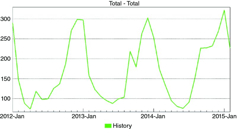
Figure 2.1 Monthly Sales for Cough Syrup Brand

Figure 2.2 Monthly Sales for Cough Syrup SKU
Many organizations that need to generate low-level forecasts discover that at the lowest levels there is not enough structure to generate meaningful statistical forecasts directly from the low-level data. In these cases there is little choice but to generate the lowest-level forecasts not with statistical models, but rather by using some type of top-down allocation scheme.
Are the Relationships Between Levels Changing in Time?
A statistical model uses past demand history to forecast how things are changing in time. If there is a relationship between two levels of your hierarchy that is time independent, then you may be able to define an allocation scheme to forecast the lower level rather than trying to forecast it based on history.
For example, a shoe manufacturer needs a forecast for a men’s running shoe for each size manufactured. The demand for the specific style of shoe is changing in time, so the shoe-level forecast should be generated using a statistical method to capture the change. On the other hand, the size of runners’ feet is not changing rapidly in time, so the by-size forecasts can be generated by allocating the shoe-level forecast to the sizes using a size distribution chart.
Another example might be an automobile manufacturer who uses a statistical model to forecast vehicle sales and then allocates via a bill of materials to generate a parts-level forecast.
In both of these examples, because the relationship between the levels is known and not changing in time, the allocation approach will likely be more accurate than trying to statistically model the lower-level data.
Summary
Deciding how to organize your forecasting hierarchy and how to forecast each level can have deep ramifications on forecast accuracy. As you make these important decisions, you need to: (1) question whether you have simplified your hierarchy as much as possible; (2) determine what levels have enough structure for you to apply statistical methods directly to the data, and (3) understand the relationships between the levels—particularly those where a logical allocation scheme could be used to generate the lower-level forecasts.
2.5 When Is a Flat-line Forecast Appropriate?5
Eric Stellwagen
A forecasting technique that generates a forecast based solely on an item’s past demand history is referred to as a time-series method. Typically, time-series methods will capture structure in the history—such as current sales levels, trends, and seasonal patterns—and extrapolate them forward.
When the data are not trended and are not seasonal, a time-series method will often generate a flat-line forecast reflecting the current sales level. Because a flat line is often an implausible scenario for the future, delivering a flat-line forecast to management may require explaining the distinction between a scenario for the future and a statistical forecast of the future. This article explains this distinction and discusses when a flat-line forecast is and is not appropriate.
Consider the two data sets shown below. Figure 2.3 represents monthly demand for an expensive spare parts assembly needed to maintain commercial equipment. Notice that the historic demand consists of integers and has equaled either 0, 1, 2, 3, or 4 units in any given month.
Figure 2.4 represents annual rainfall in a city in Brazil for the period 1849–1920. Notice that historically it has rained anywhere from 50 to 250 centimeters per year and the amount of rainfall can vary quite widely from year to year.

Figure 2.3 Monthly Demand

Figure 2.4 Annual Rainfall
Neither data set is trended. Neither data set is seasonal. Thus, their forecasts are not trended and are not seasonal—they are flat. This does not indicate that the future demand for the spare parts assembly or rainfall will be flat—these amounts will continue to fluctuate in the future—it just indicates that how these amounts will fluctuate is not predictable based solely on the historic data. The expected range of the fluctuations is shown by the confidence limits.
Let’s take a closer look at our spare parts assembly. The forecast is 0.9 units per month and the upper confidence limit is set to 97.5%. Notice that the forecast is not a possible scenario for the future—we will not sell 0.9 units per month for the next 12 months—in all likelihood we will continue to sell either 0, 1, 2, 3, or 4 units in any given month. The problem is that the timing and size of the future orders is not knowable from the past history. So what does our forecast tell us, and how do we use it?
In the statistical sense, the forecast is the expected value for the future periods. It is the point at which (according to the model) it is equally likely that the actual value will fall above or below. If we are trying to estimate expected revenue for our spare parts assembly, this is exactly what we want. We can take our forecasts and multiply them by our average selling price to determine our expected revenues. If we want to know how many spare parts assemblies to keep in inventory, we use our upper confidence limit.
Notice that even though our data are highly variable and our forecast is flat, the accuracy of the forecast and confidence limits still has a major impact on our revenue planning and inventory policies. Thus, it is important to generate the most accurate forecast possible, even when the forecast is a flat line.
2.6 Forecasting by Time Compression6
Udo Sglavo
Introduction
Demand forecasting is a challenging activity. This is particularly true for the retail industry, where more rigorous forecasting and planning processes and statistical tools are beginning to augment the “art” of merchandising and replenishment.
Retailers want to know what will sell at which price points, what promotions will be most effective, and what will be the best clearance strategy when a product is out of season. These questions all have a basis in forecasting.
Forecasting is considered an important function, and it follows the same iterative process with each forecasting and planning cycle. The process usually involves generating updated forecasts based on the most recent data, reconciling forecasts in a hierarchical manner, identifying and remedying problematic forecasts, adding judgmental overrides to the forecasts based on business knowledge, and publishing the forecasts to other systems or as reports. However, many organizations still rely solely on readily available tools that their employees are comfortable with rather than using specialized forecasting software.
Given the relatively small number of forecasters in most organizations, a large degree of automation is often required to complete the forecasting process in the time available for each planning period. Retailers still may be faced with some types of forecasts that need special consideration—for example, forecasting the demand of products that are only sold during one season, or around a holiday.
This paper will suggest an approach for dealing with these kinds of highly seasonal forecasts. It provides an illustrative example based on real-life data.
The Challenge
Retailers are commonly faced with producing predictions for items that are only sold at a certain time of the year. A typical example would be special items that are available only during a short season—such as a holiday period. The challenge for a typical retailer is to produce a forecast for these types of items, because they need to let their suppliers know in advance how many items they will need. Sometimes the lead time can be up to six months or more. Ordering too few items will result in stockouts, which lead to lost revenue and customer dissatisfaction. At the same time, ordering too many items will result in overstocks, leading to waste or costly markdowns.

Figure 2.5 Daily Sales Volume
From a statistical forecasting perspective, tackling this challenge is difficult. Most values of the underlying time series will be zero (when the product is out of season)—but there are huge sales spikes when the product is in season.
A typical graphical representation for such an item is provided in Figure 2.5. In this case, we are trying to model a special beverage, which is sold only during Easter. The data at hand is in a daily format—beginning on Monday, August 1, 2005, and ending on Thursday, July 31, 2008.
Our task is to come up with a forecast for the Easter period 2009 in weekly numbers.
Approach 1: Traditional Forecasting
As a first step, we will try to fit traditional statistical forecasting models. Because we need to provide weekly forecasts, we will first aggregate the daily data to weekly levels (see Figure 2.6). This will remove some of the random noise in the data. We also will add additional values to our time series to get complete yearly information. This can be done easily, as we know the sales before and after the Easter selling period are zero.

Figure 2.6 Weekly Sales Volume
Because no sales information was provided for Easter 2005, we will drop the year 2005 from our analysis. After doing this we can use forecasting software to come up with a decent forecasting model. In addition, we will define some events that flag the Easter holiday—hoping that this information will improve the models. For this retailer, the sales pattern of the Easter beverage always starts three weeks before Easter and continues through one week after Easter.
After using these steps, it occurs to us that while the forecasting software is capable of identifying the Easter pattern (Figure 2.7), it does not identify the sales increase accurately enough (Figure 2.8). This behavior is caused by the particular structure of our data, which contains mostly zeros.
Approach 2: Forecasting by Time Compression
Rather than trying to come up with better statistical forecasting models by fine-tuning our initial model, we want to try an alternative approach. Our idea is to compress the data by putting all dates that are zero into one bucket. Then we want to create a forecasting model based on this new time series. After forecasting we will transform the data back to its original format.

Figure 2.7 Forecast Model Generated by Forecasting Software

Figure 2.8 Model Fit Errors
Step 1: Compress Time Dimension of Original Series
To compress our original time series, we need to flag the Easter event first and then merge all observations that do not happen during the Easter event into another observation (with volume zero). Due to the structure of the sales pattern (sales occur beginning three weeks before Easter, during Easter week, and for one week after Easter), our “Easter event” bucket will consist of five points. We then compress all of the year’s time periods before the Easter event into one point (with value zero), and all time periods after that for the year into one point (with value zero). This results in seven observations per year (Figure 2.9). Note that this also indicates our seasonality pattern (which is seven).
Step 2: Create Forecasting Model and Predictions
After creating the new series we can fit traditional statistical forecasting models using our forecasting software. In our case, an additive-winters exponential method gives the most appropriate fit (Figure 2.10).
Step 3: Transforming Forecasts Back to Original Time Format
Because we know about the future Easter period, it is fairly easy to back-transform the data into its original format. Again we will assume that no sales occur outside of the selling period, and we will set these values to zero in the forecasting horizon (Figure 2.11).

Figure 2.9 Sales Volume after Compression of the Time Dimension

Figure 2.10 Forecast Model of the Compressed Volume
As we can see (Figure 2.12), our new forecasts not only identify our sales pattern accordingly; this time we get a better overall fit to history and, more important, we get better estimates of the sales spike compared to our first approach.
Conclusion
Forecasting data of highly seasonal items (items that are sold only for a short time during the year, but with large volumes) is a challenging task. Using the compression approach introduced in this paper, traditional forecasting techniques can be applied to transformed time series. Initial results seem to suggest that the accuracy of such an approach could be superior to a more standard way of time-series modeling.
Acknowledgments
The initial idea proposed in this paper was suggested by Michael Leonard, SAS Research & Development. Thanks to Mike Gilliland, SAS Marketing, Bob Lucas, SAS Education, and Snurre Jensen, SAS Denmark for valuable comments on the draft of this paper.
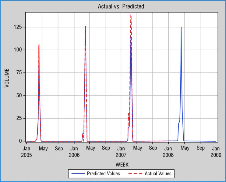
Figure 2.11 Sales and Forecast (after Transformation back to Weekly)

Figure 2.12 Model Fit Errors
REFERENCES
- Brocklebank, John C., and David A. Dickey (2003). SAS for Forecasting Time Series, Second Edition. Cary, NC: SAS Institute and John Wiley & Sons.
- Box, G. E. P, G. M., Jenkins, and G. C. Reinsel (1994). Time Series Analysis: Forecasting and Control. Englewood Cliffs, NJ: Prentice Hall, Inc.
- Makridakis, S. G., S. C. Wheelwright, and R. J. Hyndman (1997). Forecasting: Methods and Application. New York: John Wiley & Sons.
2.7 Data Mining for Forecasting: An Introduction
Chip Wells and Tim Rey
Introduction, Value Proposition, and Prerequisites
Big data means different things to different people. In the context of forecasting, the savvy decision maker needs to find ways to derive value from big data. Data mining for forecasting offers the opportunity to leverage the numerous sources of time-series data, both internal and external, now readily available to the business decision maker, into actionable strategies that can directly impact profitability. Deciding what to make, when to make it, and for whom is a complex process. Understanding what factors drive demand, and how these factors (e.g., raw materials, logistics, labor, etc.) interact with production processes or demand and change over time, are keys to deriving value in this context.
Traditional data-mining processes, methods, and technology oriented to static type data (data not having a time-series framework) have grown immensely in the last quarter century (Fayyad et al. (1996), Cabena et al. (1998), Berry (2000), Pyle (2003), Duling and Thompson (2005), Rey and Kalos (2005), Kurgan and Musilek (2006), Han et al. (2012)). These references speak to the process as well as myriad of methods aimed at building prediction models on data that does not have a time-series framework. The idea motivating this paper is that there is significant value in the interdisciplinary notion of data mining for forecasting. That is, the use of time-series based methods to mine data collected over time.
This value comes in many forms. Obviously being more accurate when it comes to deciding what to make when and for whom can help immensely from an inventory cost reduction as well as a revenue optimization view point, not to mention customer satisfaction and loyalty. But there is also value in capturing a subject matter expert’s knowledge of the company’s market dynamics. Doing so in terms of mathematical models helps to institutionalize corporate knowledge. When done properly, the ensuing equations become intellectual property that can be leveraged across the company. This is true even if the data sources are public, since it is how the data is used that creates intellectual property, and that is in fact proprietary.
There are three prerequisites to consider in the successful implementation of a data mining for time-series approach: understanding the usefulness of forecasts at different time horizons, differentiating planning and forecasting, and, finally, getting all stakeholders on the same page in forecast implementation.
One primary difference between traditional and time-series data mining is that, in the latter, the time horizon of the prediction plays a key role. For reference purposes, short-ranged forecasts are defined herein as 1 to 3 years, medium-range forecasts are defined as 3 to 5 years, and long-term forecasts are defined as greater than 5 years. The authors agree that anything greater than 10 years should be considered a scenario rather than a forecast.1 Finance groups generally control the “planning” roll up process for corporations and deliver “the” number that the company plans against and reports to Wall Street. Strategy groups are always in need for medium (1–3 years) to long range (3+ years) forecasts for strategic planning. Executive sales and operations planning (ESOP) processes demand medium range forecasts for resource and asset planning. Marketing and Sales organizations always need short to medium range forecasts for planning purposes. New business development incorporates medium to long-range forecasts in the NPV process for evaluating new business opportunities. Business managers rely heavily on short- and medium-term forecasts for their own businesses data but also need to know the same about the market. Since every penny a purchasing organization can save a company goes straight to the bottom line, it behooves a company’s purchasing organization to develop and support high-quality forecasts for raw materials, logistics costs, materials and supplies, as well as services.
However, regardless of the needs and aims of various stakeholder groups, differentiating a “planning” process from a “forecasting” process is critical. Companies do need to have a plan that is aspired to. Business leaders have to be responsible for the plan. But, to claim that this plan is a “forecast” can be disastrous. Plans are what we “feel we can do,” while forecasts are mathematical estimates of what is most likely. These are not the same, and both should be maintained. The accuracy of both should be tracked over a long period of time. When reported to Wall Street, accuracy is more important than precision. Being closer to the wrong number does not help.
Given that so many groups within an organization have similar forecasting needs, a best practice is to move toward a “one number” framework for the whole company. If Finance, Strategy, Marketing/Sales, Business ESOP, NBD, Supply Chain, and Purchasing are not using the “same numbers,” tremendous waste can result. This waste can take the form of rework and/or mismanagement given an organization is not totally lined up to the same numbers. This then calls for a more centralized approach to deliver forecasts for a corporation, which is balanced with input from the business planning function. Chase (2013) presents this corporate framework for centralized forecasting in his book Demand-Driven Forecasting.
Raw ingredients in a successful forecasting implementation are historical time-series data on the Y variables that drive business value and a selected group of explanatory (X) variables that influence them. Creating time-series data involves choosing a time interval and method for accumulation. Choosing the group of explanatory variables involves eliminating irrelevant and redundant candidates for each Y.2 These tasks are interrelated. For example, if demand is impacted by own price and prices of related substitute and complementary goods, and if prices are commonly reset about once a month, then monthly accumulation should give the analyst the best look at candidate price correlation patterns with various demand series.
The remainder of this article presents an overview of techniques and tools that have proven to be effective and efficient in producing the raw materials for a successful forecasting analysis. The context of the presentation is a large scale forecasting implementation, and Big Data—that is, thousands of Y and candidate X series, is the starting point.
Big Data in Data Mining for Forecasting
Big Data Source Overview
Over the last 15 years or so, there has been an explosion in the amount of external time series based data available to businesses. Commercial sources include: Global Insights, Euromonitor, CMAI, Bloomberg, Nielsen, Moody’s, Economy.com, and Economagic. There are also government sources such as: www.census.gov, www.stastics.gov.uk/statbase, IQSS database, research.stlouisfed.org, imf.org, stat.wto.org, www2.lib.udel.edu, and sunsite.berkeley.edu. All provide some sort of time-series data—that is, data collected over time inclusive of a time stamp. Many of these services are for a fee; some are free. Global Insights (ihs.com) alone contains over 30,000,000 time series.
This wealth of additional information actually changes the way a company should approach the time-series forecasting problem in that new methods are necessary to determine which of the potentially thousands of useful time series variables should be considered in the exogenous variable forecasting problem. Business managers do not have the time to “scan” and plot all of these series for use in decision making.
Many of these external sources offer databases for historical time-series data but do not offer forecasts of these variables. Leading or forecasted values of model exogenous variables are necessary to create forecasts for the dependent or target variable. Other services, such as Global Insights, CMAI, and others, do offer lead forecasts.
Concerning internal data, IT Systems for collecting and managing data, such as SAP and others, have truly opened the door for businesses to get a handle on detailed historical static data for revenue, volume, price, costs, and could even include the whole product income statement. That is, the system architecture is actually designed to save historical data. Twenty-five years ago, IT managers worried about storage limitations and thus would “design out of the system” any useful historical detail for forecasting purposes. With the cost of storage being so cheap now, IT architectural designs have included “saving” various prorated levels of detail so that companies can take full advantage of this wealth of information.
Relevant Background on Time-Series Models
A couple of important features about time-series modeling are important at this point. First, the one thing that differentiates time-series data from simple static data is that the time-series data can be related to “itself” over time. This is called serial correlation. If simple regression or correlation techniques are used to try and relate one time series variable to another, and ignore possible serial correlation, the businessperson can be misled. So, rigorous statistical handling of this serial correlation is important.
The second feature is that there are two main classes of statistical forecasting approaches to consider. First there are univariate forecasting approaches. In this case, only the variable to be forecast (the Y or dependent variable) is considered in the modeling exercise. Historical trends, cycles, and seasonality of the Y itself are the only structures considered when building the forecasting model. There is no need for data mining in this context.
In the second approach—where the plethora of various time-series data sources comes in—various X or independent (exogenous) variables are used to help forecast the Y or dependent variable of interest. This approach is considered exogenous variable forecast model building. Businesses typically consider this value added; now we are trying to understand the drivers or leading indicators. The exogenous variable approach leads to the need for data mining for forecasting problems.
Though univariate or Y-only forecasts are often times very useful, and can be quite accurate in the short run, there are two things that they cannot do as well as the multivariate forecasts. First and foremost is providing an understanding of “the drivers” of the forecast. Business managers always want to know what “variables” (and in this case means what other time-series) “drive” the series they are trying to forecast. Y-only forecasts do not accommodate these drivers. Second, when using these drivers, the exogenous variable models can often forecast further and more accurately than the univariate forecasting models.
The recent 2008/2009 recession is evidence of a situation where the use of proper Xs in an exogenous variable leading-indicator framework would have given some companies more warning of the dilemma ahead. Univariate forecasts were not able to capture this phenomenon as well as exogenous variable forecasts.
The external databases introduced above not only offer the Ys that businesses are trying to model (like that in NAICS or ISIC databases), but also provide potential Xs (hypothesized drivers) for the multivariate (in X) forecasting problem. Ellis (2005) in “Ahead of the Curve” does a nice job of laying out the structure to use for determining what X variables to consider in a multivariate in X forecasting problem. Ellis provides a thought process that, when complemented with the data mining for forecasting process proposed herein, will help the business forecaster do a better job identifying key drivers as well as building useful forecasting models.
The use of exogenous variable forecasting not only manifests itself in potentially more accurate values for price, demand, costs, etc. in the future, but it also provides a basis for understanding the timing of changes in economic activity. Achuthan and Banerji (2004), in Beating the Business Cycle, along with Banerji (1999), present a compelling approach for determining potential Xs to consider as leading indicators in forecasting models. Evans et al. (2002) as well (www.nber.org and www.conference-board.org) have developed frameworks for indicating large turns in economic activity for large regional economies as well as specific industries. A part of the process they outline identifies key drivers. In the end, much of this work speaks to the concept that, if studied over a long enough time frame, many of the structural relations between Y and X are fairly stable. This offers solace to the business decision maker and forecaster willing to learn how to use data mining techniques for forecasting in order to mine the time-series relationships in the data.
Many large companies have decided to include external data, such as that found in Global Insights as mentioned above, as part of their overall data architecture. Small internal computer systems are built to automatically move data from the external source to an internal database. This, accompanied with tools used to extract internal static data, allows bringing both the external Y and X data alongside the internal. Oftentimes the internal Y data are still in transactional form. Once properly processed, or aggregated, e.g., by simply summing over a consistent time interval like month and concatenated to a monthly time stamp, this time stamped data becomes time-series data. This database would now have the proper time stamp, include both internal and external Y and X data, and be all in one place. This time-series database is now the starting point for the data mining for forecasting multivariate modeling process.
Feature Selection: Origins and Necessary Refinements for Time Series
Various authors have defined the difference between data mining and classical statistical inference; Hand (1998), Glymour et al. (1997), and Kantardzic (2011) are notable examples. In a classical statistical framework, the scientific method (Cohen and Nagel, 1934) drives the approach. First, there is a particular research objective sought after. These objectives are often driven by first principles or the physics of the problem. This objective is then specified in the form of a hypothesis; from there a particular statistical “model” is proposed, which then is reflected in a particular experimental design. These experimental designs make the ensuing analysis much easier in that the Xs are independent, or orthogonal to one another. This othogonality leads to perfect separation of the effects of the “drivers” therein. So, the data are then collected, the model is fit, and all previously specified hypotheses are tested using specific statistical approaches. Thus, very clean and specific cause and effect models can be built.
In contrast, in many business settings a set of “data” often times contains many Ys and Xs, but has no particular modeling objective or hypothesis for being collected in the first place. This lack of an original objective often leads to the data having irrelevant and redundant candidate explanatory variables. Redundancy of explanatory variables is also known as multicollinearity—that is, the Xs are actually related to one another. This makes building cause-and-effect models much more difficult. Data mining practitioners will “mine” this type of data in the sense that various statistical and machine learning methods are applied to the data looking for specific Xs that might “predict” the Y with a certain level of accuracy. Data mining on static data is then the process of determining what set of Xs best predicts the Y(s). This is a different approach than classical statistical inference using the scientific method. Building adequate prediction models does not necessarily mean an adequate cause-and-effect model was built.
Considering time-series data, a similar framework can be understood. The scientific method in time-series problems is driven by the “economics” or “physics” of the problem. Various “structural forms” may be hypothesized. Often times there is a small and limited set of Xs, which are then used to build multivariate times-series forecasting models or small sets of linear models that are solved as a “set of simultaneous equations.” Data mining for forecasting is a similar process to the “static” data-mining process. That is, given a set of Ys and Xs in a time-series database, what Xs do the best job of forecasting the Ys? In an industrial setting, unlike traditional data mining, a “data set” is not normally readily available for doing this data mining for forecasting exercise. There are particular approaches that in some sense follow the scientific method discussed earlier. The main difference herein will be that time-series data cannot be laid out in a designed-experiment fashion.
With regard to process, various authors have reported on data mining for static data. A paper by Azevedo and Santos (2008) compared the KDD process, SAS Institute’s SEMMA process (Sample, Explore, Modify, Model, Assess), and the CRISP data-mining process. Rey and Kalos (2005) review the data-mining and modeling process used at the Dow Chemical Company. A common theme in all of these processes is that there are many candidate explanatory variables, and some methodology is necessary to reduce the number of Xs provided as input to the particular modeling method of choice. This reduction is often referred to as Variable or Feature selection. Many researchers have studied and proposed numerous approaches for variable selection on static data (Koller and Sahami (1996), Guyon and Elisseeff (2003), etc.). One of the expositions of this article is an evolving area of research in variable selection for time-series type data.
NOTES
REFERENCES
- Achuthan, L., and A. Banerji (2004). Beating the Business Cycle. New York: Doubleday.
- Azevedo, A., and M. Santos (2008). KDD, SEMMA and CRISP-DM: A Parallel Overview. Proceedings of the IADIS.
- Banerji, A. (1999). The lead profile and other nonparametrics to evaluate survey series as leading indicators. 24th CIRET Conference.
- Berry, M. (2000). Data Mining Techniques and Algorithms. Hoboken, NJ: John Wiley & Sons.
- Cabena, P., P. Hadjinian, R. Stadler, J. Verhees, J., and A. Zanasi (1998). Discovering Data Mining: From Concept to Implementation. Englewood Cliffs, NJ: Prentice Hall.
- Chase, C. (2013). Demand-Driven Forecasting (2nd ed.). Hoboken, NJ: John Wiley & Sons.
- Cohen, M., and E. Nagel (1934). An Introduction to Logic and Scientific Method. Oxford, England: Harcourt, Brace.
- CRISP-DM 1.0, SPSS, Inc., 2000.
- Data Mining Using SAS Enterprise Miner: A Case Study Approach. Cary, NC: SAS Institute, 2003.
- Duling, D., and W. Thompson (2005). What’s New in SAS® Enterprise Miner™ 5.2. SUGI-31, Paper 082–31.
- Ellis, J. (2005). Ahead of the Curve: A Commonsense Guide to Forecasting Business and Market Cycles. Boston, MA: Harvard Business School Press.
- Evans, C., C. Liu, and G. Pham-Kanter (2002). The 2001 recession and the Chicago Fed National Activity Index: Identifying business cycle turning points. Economic Perspectives 26(3):26–43.
- Fayyad, U., G. Piatesky-Shapiro, P. Smyth, and R. Uthurusamy (eds.). (1996). Advances in Knowledge Discovery and Data Mining. AAAI Press.
- Glymour, C. et al. (1997). Statistical themes and lessons for data mining. Data Mining and Knowledge Discovery 1, 11–28. Netherlands: Kluwer Academic Publishers.
- Guyon, I., and A. Elisseeff (2003). An introduction to variable and feature selection. Journal of Machine Learning Research 3 (3), 1157–1182.
- Han, J., M. Kamber, and J. Pie (2012). Data Mining: Concepts and techniques. Amsterdam: Elsevier, Inc.
- Hand, D. (1998). Data mining: Statistics and more? The American Statistician 52 (2), 112–118.
- Kantardzic, M. (2011). Data Mining: Concepts, Models, Methods, and Algorithms. Piscataway, NJ: IEEE Press.
- Koller, D., and M. Sahami (1996). Towards optimal feature selection. International Conference on Machine Learning 284–292.
- Kurgan, L., and P. Musilek (2006). A survey of knowledge discover and data mining process models. The Knowledge Engineering Review 21 (1), 1–24.
- Pyle, D. (2003). Business modeling and data mining. Elsevier Science.
- Rey, T., and A. Kalos (2005). Data mining in the chemical industry. Proceedings of the Eleventh ACM SIGKDD.
2.8 Process and Methods for Data Mining for Forecasting
Chip Wells and Tim Rey
This article provides a framework and overview of various methods for implementing a data mining for forecasting analysis (see Figure 2.13). Further details on process and methodologies as well as step-by-step applied examples are given in Rey et al. (2012), Applied Data Mining for Forecasting Using SAS®.
The process for developing time-series forecasting models with exogenous variables starts with understanding the strategic objectives of the business leadership sponsoring the project.
This is often secured via a written charter so as to document key objectives, scope, ownership, decisions, value, deliverables, timing, and costs. Understanding the system under study with the aid of the business subject-matter experts provides the proper environment for focusing on and solving the right problem. Determining from here what data help describe the system previously defined can take some time. In the end, it has been shown that the most time consuming step in any data-mining prediction or forecasting problem is in the data processing step where data is created, extracted, cleaned, harmonized, and prepared for modeling. In the case of time-series data, there is often a need to harmonize the data to the same time frequency as the forecasting problem at hand.

Figure 2.13 Model Development Process
Time-Series Data Creation
A key element in the process illustrated above is the selection of the time interval and accumulation method for analysis. Various stakeholder groups will have preferred intervals and summary methods that integrate well with their planning and reporting processes. However, the selection of the interval and method of implementation for time-series data mining and subsequent modeling should be based on the answer to the following question; What roll-up method yields the best “look” at systematic patterns of interest in the data? These include price effects, seasonality, technological cycles, and so on.
A fact that forecast stakeholder groups sometimes fail to fully appreciate is that the data are created in the process of a time-series analysis. Choices of an accumulation (transformation of time stamped into time-series data) and aggregation (creation of time-series hierarchies) intervals impact underlying patterns that determine the forecastability (or not) of data that flow into the models. For example, if prices are reset about once a week, but the selected interval is month or quarter, then variation in prices would likely be overly smoothed, and the forecastability of the data may be diminished.
Further, a roll-up method must be chosen. Total (sum) usually works well to construct an observation of units of demand per interval, and average is a reasonable choice for prices. However, the analyst must understand the data, and choose a method that will provide a conduit for systemic patterns to be emphasized in the time series. For example, inventories at levels around historical averages may have very little impact on demand. However, very low or high inventory levels may strongly influence customer behavior. A better accumulation method may be the maximum or minimum observation in a given interval in this case.
Given an interval and roll-up method, there is often a need to handle missing values. This may be in the form of forecasting forward, back casting, or simply filling in missing data points with various algorithms. So, just as in data mining for static data, a specific imputation method is needed.1
Three methods for input variable reduction and selection in a time-series setting are outlined below. In application, any one is usually implemented in an iterative way. That is, an accumulation interval and method are proposed, and a given method is run. Results are assessed for plausibility, correlation strength, and robustness by analysts and subject matter experts. Given the time available and the value of the series to be forecast, alternative intervals and methods are tried. The end goal is to find an interval and accumulation method that leads to the selection of unique explanatory variables whose variation is strongly correlated with and that leads variation in the Y variables.
Two Phases of Data Mining for Forecasting
The initial phase of the analysis is centered on the variable reduction step. In variable reduction, subject matter expertise is combined with various approaches (see below) to reduce the number of Xs being considered while at the same time “explaining” or “characterizing” the key sources of variability in the Xs regardless of the Ys. The goal is to reduce a large group of, possibly, thousands of candidate X variables down to a group size of a couple hundred. Stakeholders with knowledge of the data are instrumental here in helping analysts understand how variables are denominated and derived, what variables are truly redundant (e.g., different names for the same thing), and what Xs are hypothesized to play key roles within various business lines and regions.
The later phase of a data mining for forecasting analysis is focused on variable selection. Variable selection relies more heavily on algorithms, and this step contains supervised methodologies since the Ys are now being considered. Various methods (some are outlined later) assess the candidate Xs for correlation with the Ys. If a correlation exists, further steps are centered on identifying its dynamic structure (e.g., contemporaneous, lead, or delay). Subject-matter experts continue to play a role in variable selection. Their judgment in assessing the magnitude, robustness, and plausibility of automated feature selection algorithm results is a final sanity check that helps to ensure forecasts are as precise as possible.
Three Methods for Data Mining in Time Series
One of the key problems with using static variable reduction and variable selection approaches on time-series data are that, in order to overcome the method not being time-series based, the modeler has to include lags of the Xs in the problem. This dramatically increases the size of the variable selection problem. For example, if there are 1,000 Xs in the problem, and the data interval is quarter, the modeler would have to add a minimum of four lags for each X in the variable reduction or selection phase of the project. This is because the Y and X are potentially correlated at any or all positive lags of Y on X, 1 to 4, and thus now there are 4,000 “variables” to be processed.
In the traditional data-mining literature on static or “non” time-series data, many researchers have proposed numerous approaches for variable reduction and selection on static data (again Koller and Sahami (1996), Guyon and Elisseeff (2003), etc.). The serially correlated structure and the potential for correlation between candidate Xs and Ys at various lags makes implementing traditional data mining techniques on time-series data problematic. New techniques are necessary for dimension reduction and model specification that accommodate the unique aspects of the problem. Below, we present three methods that have been found to be effective for mining time-series data.
A similarity analysis approach can be used for both variable reduction and variable selection. Leonard et al. (2008) introduce an approach for analyzing and measuring the similarity of multiple time-series variables. Unlike traditional time-series modeling for relating Y (target) to an X (input) similarity analysis leverages the fact that the data is ordered. A similarity measure can take various forms but essentially is a metric that measures the distance between the X and Y sequences keeping in mind ordering. Similarity can be used simply to get the similarity between the Ys and the Xs but it can also be used as input to a variable clustering algorithm to then get clusters of Xs to help reduce redundant information in the Xs and thus reduce the number of Xs.
1. A cointegration approach for variable selection is implemented. Engle and Granger (2001) discuss a cointegration test. Cointegration is a test of the economic theory that two variables move together in the long run. The traditional approach to measuring the relationship between Y and X would be to make each series stationary (generally by taking first differences) and then see if they are related using a regression approach. This differencing may result in a loss of information about the long-run relationship. Differencing has been shown to be a harsh method for rendering a series stationary. Thus cointegration takes a different tack. First, the simple OLS regression model (called the cointegrating regression), where X is the independent variable, Y is the dependent variable, t is time, α and β are coefficients, and is the residual. The actual test statistic used to see if the residuals of the model are stationary is either the Dickey-Fuller test or the Durbin Watson test. In the implementation examples below the Dickey-Fuller test is used.
2. A cross-correlation approach for variable selection is described. A common approach used in time-series modeling for understanding the relationship between Y and X is called the cross-correlation function (CCF). A CCF is simply the bar chart of simple Pearson product moment correlations for each of the lags under study.
3. We have automated all of these methods and combine them into one table for review by the lead modeler and a panel of subject matter experts (see Table 2.14).
In these big data, time-series variable reduction and variable selection problems, we combine all three, along with the prioritized list of variables the business SMEs suggest, into one research database for studying (see Table 2.15).
Next, various forms of time-series models are developed; but, just as in the data mining case for statics data, there are some specific methods used to guard against overfitting that help provide a robust final model. This includes, but is not limited to, dividing the data into three parts: model, hold out, and out of sample. This is analogous to training, validating, and testing data sets in the static data-mining space. Various statistical measures are then used to choose the final model. Once the model is chosen, it is deployed using various technologies.
First and foremost, the reason for integrating data mining and forecasting is simply to provide the highest quality forecasts as possible. The unique advantage to this approach lies in having access to literally thousands of potential Xs and now a process and technology that enables doing the data mining on time-series type data in an efficient and effective manner. In the end, the business receives a solution with the best explanatory forecasting model as possible. With the tools now available through various technologies, this is something that can be done in an expedient and cost efficient manner.
Now that models of this nature are easier to build, they can then be used in other applications inclusive of scenario analysis, optimization problems, as well as Simulation problems (linear systems of equations as well as nonlinear system dynamics). So, all in all, the business decision maker will be prepared to make better decisions with these forecasting processes, methods, and technologies.

Figure 2.14 Table Prepared for Review

Figure 2.15 Research Database
NOTE
REFERENCES
- Engle, R., and W. Granger (2001). Long-Run Economic Relationships: Readings in Cointegration. New York: Oxford University Press.
- Guyon, I., and A. Elisseeff (2003). An introduction to variable and feature selection. Journal of Machine Learning Research 3 (3), 1157–1182.
- Koller, D., and M. Sahami (1996). Towards optimal feature selection. International Conference on Machine Learning 284–292.
- Leonard, M., T. Lee, J. Sloan, and B. Elsheimer (2008). An introduction to similarity analysis using SAS®. SAS Institute White Paper.
- Rey, T., A. Kordon, and C. Wells (2012). Applied Data Mining for Forecasting Using SAS®. Cary, NC: SAS Institute Inc.
2.9 Worst-Case Scenarios in Forecasting: How Bad Can Things Get?7
Roy Batchelor
Worst-Case Damage from a Blowout in the Gulf of Mexico
According to news reports, the main contingency plan foresaw a blowout with a worst-case spill of 40 million gallons in total. During the first three months, millions of gallons have been gushing per day. Regulatory agencies based their efforts on worst-case scenarios that weren’t nearly worst case.
Introduction
Throughout the recent recession, companies have watched sales and production shrink by unprecedented amounts. Month after month, outturns have not merely fallen short of central forecasts but have crashed through the lower limits of prediction intervals churned out by statistical models. Conventional business-forecasting systems are just not set up to tell us about extreme events.
Downside risk has long been a central concern of financial forecasters. In the financial markets, high volatility in prices means large potential losses for investors, and risk-averse hedgers will pay more for insurance against adverse events. Option pricing theory ties the cost of insurance directly to the forecast of volatility of future price changes. A massive academic and practitioner literature has sprung up, focused on getting good predictions of whether share prices, currencies, and commodities are likely to become more or less volatile in the future.
Volatility changes can be forecast. Day-to-day price changes are close to random, but the volatility of these price changes is serially correlated: If there is a big price change (up or down) on one day, it is more likely than not that there will be a big price change the following day (down or up, we don’t know which).
More recently, downside risk has become an important issue for business forecasters who are concerned with future sales, rather than prices on the financial markets. Most companies try to define worst-case scenarios for sales. Models of inventory control rely heavily on estimates of the future volatility of demand. Yet somehow, the well-developed technology of volatility forecasting has not been transferred into the business domain. To see what that would involve, I have set out below the procedure for defining a worst-case scenario that would follow from reading a basic business forecasting text. Then I illustrate how the transfer of a small piece of volatility forecasting technology—the GARCH variance model—from a financial to a business-forecasting environment can help quantify downside risk.
A Standard View of New Car Sales
Consider the point of view of a forecaster trying to predict new-car sales in the U.S. through the 2008–2009 recession. Imagine we are in early September 2008. We have a preliminary estimate of August sales of around 630 thousand vehicles. This was about 10% lower than August of a year earlier, but still well within the range of 500–800 thousand that had been the norm since 2000. Visual inspection of the monthly data on Figure 2.16 suggests that a worst-case scenario would be monthly sales below 500 thousand, an event that happened in only three of the previous 103 months.
To generate a forecast for September 2008 onwards, we need a model for car sales. I have used a conventional time-series representation using data back to 1980, a seasonal ARIMA model. The forecasts from this model are shown on Figure 2.17, in the form that is generated by most standard business-software packages. This shows expected sales (light gray line) and upper and lower bounds to the 95% prediction interval. The idea is that, in 95% of forecast months, sales should lie within these limits. Sales are forecast to be around 600 thousand cars per month, with some seasonal fluctuations. The bad case is for sales to fall below 494 thousand in September. The estimated reliability of the central forecast is reflected in its standard error, which we could loosely define as the size of a typical monthly error. Larger values of the standard deviation imply less reliability. This lower bound is around two standard errors below the expected level of sales, so the standard error of our one-month-ahead forecast is about ½ × (600 – 494) = 53 thousand cars, or about 9% of the central forecast.

Figure 2.16 New Car Sales, January 2000–August 2008 (thousands)
What actually happened in September 2008, the month of the Lehman bankruptcy, was that consumer confidence plummeted, spending contracted across the economy, and car sales fell to an all-time low of 481 thousand, below the model’s bad-case estimate. Of course, we expect there to be two to three months in every decade when sales fall below the lower prediction bound. This was an extreme adverse event, and leads to our key question: Given such a shock, how much worse can things get?

Figure 2.17 Forecasts and Outturn for September 2008
Let’s stick with our conventional model and make a new set of forecasts for October 2008 and beyond, in light of information about the collapse in sales in September. The new path of expected sales and lower bound to the 95% prediction interval are shown in Figure 2.18. Sales are predicted to rebound to 505 thousand and then continue along a path somewhat lower than had been forecast a month earlier. Very sensibly, part of the fall in sales in September is treated as a temporary effect that will be offset in the following month, and part is treated as a signal that the underlying level of the series has permanently fallen.
Less sensible is what happens to the prediction interval. The bad case is now for sales to be 413 thousand. This is 92 thousand below the mean forecast, suggesting a standard error of 92/2 = 46 thousand. This is actually lower than a month earlier, and still only 9% of the new mean forecast. So, after the worst shock to car sales in living memory, the standard business-forecasting model suggests that our forecasts will be just as reliable as they were before the shock happened!
To underline how unrealistic this is, Figure 2.18 also shows that sales in October again fell below the model-generated lower prediction bound. Two successive outcomes below the lower bound is a very unusual occurrence and should make us reconsider how our bad-case forecast has been constructed. We could keep going—but, month after month, the standard error of the one-month-ahead forecast would stay stuck at about 9% of the forecast level, regardless of whether the economic conditions were calm or stormy.

Figure 2.18 Forecasts and Outturn for October 2008
Time-Varying Volatility in Car Sales
The problem is that conventional time-series and regression models assume that the distribution of shocks to the system stays unchanged over time. Sometimes shocks are large and sometimes small, but these are treated as random draws from an underlying probability distribution that has a constant volatility. Prediction intervals from these models are based on an estimate of the average volatility of residuals over the whole sample used in model estimation. When a new observation appears, no matter how extreme it is, it has only a marginal effect on the estimated variance of residuals, and hence scarcely affects prediction intervals.
This assumption of constant volatility of shocks—called homoscedasticity—is not one that would be entertained in any model of financial markets, where it is plain that periods of steady growth in markets are punctuated by booms and crashes, during which volatility rises sharply. Since the Nobel Prize–winning economist Rob Engle developed the so-called ARCH (autoregressive conditional heteroscedasticity) model in the 1980s, it has become standard to characterize financial time series by some variant of this model. Financial economists are also reluctant to assume that shocks are normally distributed, preferring fat-tailed distributions such as the t-distribution, which allow extreme events to occur more frequently than suggested by the normal curve.
In the most popular “generalized ARCH” or GARCH model, there is some long-term underlying average variance, but in the short term the variance of potential shocks can rise above this underlying level if there is an unexpectedly large shock (= large forecast error) to the series being modeled. I describe the GARCH model in the article appendix.
Regression packages churn out tests for normality in residuals (Jarque Bera test) and for ARCH errors (Engle’s Lagrange multiplier test). These are often ignored because they do not bias central forecasts. They are critical, however, for constructing prediction intervals. Therefore, we can easily test whether shocks to car sales can be described by a GARCH model and whether their distribution contains more extreme events than normal. The answer is yes, and yes. Volatility in car sales does rise after unusually large and unexpected increases and decreases in sales. When shocks occur, there are more large changes than the normal curve would lead us to expect.
Let’s revisit the forecasts for September and October 2008, using the same ARIMA model for car sales but allowing the distribution of shocks to be fat-tailed and have time-varying volatility. Figure 2.19 shows the effect of the GARCH assumption on the mean forecast and the lower prediction interval bound. The mean forecast is unchanged. However, the large shock that occurred in September 2008 has caused the model to revise sharply upward its estimate of the likely volatility of future shocks. The lower prediction bound for October is now 386 thousand, much lower than the 413 thousand estimated by the conventional model.

Figure 2.19 Lower 95% Prediction Bounds: Conventional vs. GARCH
The outturn of 400 thousand is now inside rather than outside the prediction interval, and in that sense is less surprising. The fact that the October outturn is well below its expected value also means that, when we make our forecast for November, the GARCH model will again predict that volatility will be high, the prediction interval will be large, and the bad case will again be pretty bad.
Figure 2.20 shows the GARCH model estimates of how the standard deviation of shocks in the car market has changed from month to month since 2000. Although the average volatility is indeed around 9%, it can change drastically from year to year, and the very steep rise to over 15% in the recent recession shows that models of car sales that neglect changes in volatility provide us with a very poor guide to the risks faced by producers and dealers.
Note, by the way, that the most recent peak in volatility was due not to a collapse in sales, but to the splurge of buying in August 2009 in response to the “cash for clunkers” scheme that subsidized the replacement of old cars by new, more fuel-efficient vehicles.
Concluding Remarks
I have looked here at just one way of refining estimates of prediction intervals, using a simple model of time-varying volatility. There are many other ingenious devices for looking at downside risk in the financial-risk manager’s toolkit. For example, some analysts ignore all but the most extreme events and use special extreme value distributions to approximate the shape of the left tail of probability distributions. These methods are viable only if we have many observations on extreme events, and this in turn depends on the availability of high frequency, daily, or intraday data over a long time period—conditions that rule out most mainstream business-forecasting applications.

Figure 2.20 GARCH Estimates of a Time-Varying Volatility (Standard Deviation) of New-Car Sales
Business forecasters don’t often take prediction intervals seriously and have some incentives to keep quiet about them. Most of the time, the intervals look very scary. With moderate sample sizes, the conventional 95% prediction interval for three to four steps ahead typically encompasses the whole range of historic data, and colleagues and clients might be tempted to conclude that you are saying, “Anything can happen.”
Unfortunately, this is true. Indeed, results from forecasting competitions consistently tell us that, if anything, statistical prediction intervals are too narrow, since we can rarely identify the true model driving our data, and all series are subject to unforecastable structural change.
Frank Sinatra had the lyric “The best is yet to come” inscribed on his tombstone. When forecasting extreme events, it is important to understand, as well, that the worst is yet to come. The worst thing that has already happened in the sample is an upper estimate of the worst thing that can possibly happen. The honest answer to the question “How bad can things get?” is that they can always be worse than they have ever been before.
The value of models with time-varying volatility is that they help us quantify exactly how much worse things can get: whether right now we are confronted with a low or a normal degree of risk, or whether—as in September 2008—volatility is unusually high, and one of these unprecedentedly bad outcomes is most likely to occur.
Appendix: The GARCH Model
Suppose we are using time-series data to forecast a target variable yt, based on a set of predictors xt. Our standard regression model is yt = bxt + ut where b is a vector of coefficients, and the ut are regression residuals (“shocks” that cannot be explained by the predictors x). The standard assumption is that the ut are normally distributed and have a standard deviation σ that is constant over time.
The GARCH model allows σ to vary over time. Specifically, if at time t – 1 there was a big shock (so the squared residual ut-12 is large), then volatility σ will rise. Conversely, if the last residual was small, then σ will fall. The exact formula used is σt2 = a0 + a1ut-12 + a2σt-12. The larger the size of a1 relative to a2, then the greater the influence will be of the latest shock on our new estimate of volatility. The closer a2 is to 1, the more long-lived will be the effect of a large shock on the volatility of Y in subsequent time periods.
The distribution of the shocks ut need not be normal, and in the case of car sales follows a t-distribution with 8 degrees of freedom, showing that there are many more extreme events. In this case, the 95% prediction interval is not ±2σ, but ±2.3σ, making the margin of uncertainty wider and the worst-case scenario even worse.
For the U.S. car market, a1 is 0.2 and highly significant, meaning that an unexpected 10% fall in sales leads to a rise of √(0.2*0.12) = 4.5% in the standard deviation of car sales in the following month. Therefore, if volatility had been around 8% of sales, an unexpected 10% fall in sales would cause volatility to rise to 12.5% of car sales—exactly what happened between September and October 2008.
The coefficient a2 is 0.6, so the shock has a half-life of 1/(1 – 0.6) = 2.5 months. That is, after the initial large impact of the shock, in the absence of further shocks volatility will die away toward a baseline level quite quickly over the following months.
There are many variants of the GARCH model. With car sales, reactions to good news and bad news are the same. This is why volatility rose after the unexpected surge in sales in August 2009. However, with stock prices, a large fall in the market increases volatility much more than a large rise, so when modeling the stock market the coefficient a1 would be higher for negative shocks than for positive shocks.
A relatively nontechnical review of GARCH is given in Robert Engle (2001), “GARCH 101: The Use of ARCH/GARCH Models in Applied Econometrics,” Journal of Economic Perspectives 15 (4), 157–168, downloadable at http://pages.stern.nyu.edu/~rengle/Garch101.doc.
2.10 Good Patterns, Bad Patterns8
Roy Batchelor
Introduction
When a disruptive event occurs, our natural reaction is to try to predict its impact by looking for analogies whose outcomes are known. In the financial markets, this is the basis for the event study methodology that analysts have used for over 40 years to predict the effects of corporate actions like takeovers and bond downgrades. In this article, we describe the method and look at whether and how it can be extended to mainstream business and economic forecasting problems. The key to success is finding the right analogies, which in turn requires a judicious blend of domain knowledge and data mining.
Good Patterns
Suppose we want to know what is likely to happen to the share price of a particular company before and after a takeover bid. There are unlikely to be similar events in the past history of the company, and share prices are in any case very volatile. In this situation, time-series analysis and causal model building are not of much use. However, many other companies have been subjected to takeover bids in the past, and we can learn by pooling data from these episodes and searching these data for patterns. This is the basis for the highly influential and intuitively appealing event study methodology introduced by Fama, Fisher, Jensen, and Roll (1969) and surveyed by John Binder (1998).
The idea is to collect share-price data on a sample of target companies for the days before and after the takeover announcement and line up these share-price windows to see if any patterns are apparent. Figure 2.21 illustrates the results of this process, for a small sample of five companies. The gray lines show the (excess = risk-adjusted) returns that an investor in each of these companies would have made by buying the shares 60 days ahead (day −60) of the takeover announcement (on day 0).

Figure 2.21 Excess Returns for Five Takeover Targets
The experiences of the companies differ, but by averaging these returns we can see a pattern emerge, shown by the black line in the figure. Typically, there are no excess returns to be made until about 20 days before the takeover announcement, when returns gradually rise to around 10%. On the day of the announcement, share prices jump sharply by an additional 20%, and remain stable thereafter. This is why many hedge funds invest a lot of time and ingenuity in trying to identify potential takeover targets. It also explains why regulatory agencies try to identify and prosecute the insiders whose actions must be responsible for driving prices up before the public announcement of the takeover.
This is a straightforward and intuitive approach to forecasting, and we see examples in many other contexts, with varying degrees of sophistication. At the high-tech end of the forecasting business, statisticians trying to make sense of long but apparently erratic time series use nearest neighbor methods to look at the past history of the series to make forecasts based on patterns closest to those observed in the recent past. In organizations with sales and inventory data on many products, there are demonstrable benefits to pooling data for products that are related, especially if we weight these according to their similarity to the product we are trying to forecast (Duncan and colleagues, 2001). In the very practical business of figuring out the likely path for sales of new pharmaceutical or electronics products, planners often line up the sales paths following earlier launches of similar products and conjecture that the new product will follow a similar trajectory.
Bad Patterns
In the wrong hands, however, pattern-based forecasts can go horribly astray. The problem lies in knowing which prior events are genuinely analogous to the current forecasting problem. To illustrate, here are two examples of bad uses of a good methodology. In the first, data have been used uncritically, and not enough judgment has been applied. In the second, too much (biased) judgment has been applied, allowing forecasters to ignore relevant but unwelcome data.
Example 1: Not Enough Judgment
Since recession hit in 2008, newspapers and the blogosphere have been full of pictures trying to chart the likely progress of output and employment by looking at past recessions. Figure 2.22 provides a chart of U.S. nonfarm employment published on a website in February 2009. The lines show employment in the 60 months following the peak of each postwar U.S. business cycle. The path of employment in 2008 is shown by the firm black line, and the hope of the author was that previous patterns would give some guidance as to where it will go in 2009 and beyond.

Figure 2.22 U.S. Nonfarm Employment and Forecast
On the basis of the observation that employment bounced back healthily in previous recessions, the author—no names will be mentioned—wrote:
. . . a forecast of job losses continuing for another 6 to 9 months would not be out of line. Furthermore, looking at past cycles, one would expect it will be at least a year (possibly more if the recovery looks more like that after the 2001 recession) before employment reaches the previous peak. Personally, my expectation is that it will take 18 to 24 months (from now) to get back to the previous peak.
In other words, recovery was projected to follow the dashed line (two short dashes between a long dash) in the figure. What actually happened is shown by the black dashed line. Employment continued to fall, and at this time of writing—four years after the recession hit—is still almost 5% below its peak.
The problem here is that the current recession in the U.S. is not analogous to past U.S. recessions, most of which were driven by monetary policy or oil prices. How is this recession a different animal? In their fine book This Time Is Different, Reinhart and Rogoff (2009) look across financial crises in many countries in a longer sweep of history. They show that because the current crisis is driven by a failure of credit, better analogies can be found in the depressing experiences of Japan after its stock-market collapse, the Scandinavian economies after their banking crises in the 1990s, and the earlier travails of indebted emerging economies in Asia and South America. In short, the error in Figure 2.22 is that not enough judgment or theorizing has gone into choosing the sample of analogous events.
Sometimes we can get away with being sloppy about this. Consider a hedge fund that has identified some pattern predictive of a takeover. Each takeover has unique elements, and while analysts try to control for these, there will be instances where returns are lower than forecast, and others where returns are higher, and many cases where no takeover occurs. However, there will be many takeovers during the year, and the fund can act on the average patterns uncovered by its model, knowing that idiosyncratic behavior of individual shares will average out over a series of investments.
This kind of diversification of risk in forecast errors is not always possible, and definitely not in the case of costly one-off events like recessions. Similarly, the whole viability of a company may rest on the success of a single new product. When no diversification of risk is possible, the potential loss from an incorrect model is greater and possibly grievous. In these cases, a lot more attention needs to be paid to whether the events being pooled are truly analogous to the company’s product launch.
Example 2: Not Enough Data
The more care we take in finding exact analogies to the event we are trying to predict, the less hard data remain to be used, and the more we must rely on judgment rather than statistical analysis. As reported frequently in Foresight articles, judgment is not always as reliable as judges assume, and experts are rarely as expert as we would like. Good judgment—as in the Reinhart and Rogoff study—needs to be grounded in a coherent and data-congruent theory. Bad judgment is the result of belief, wishful thinking, and anecdote.
In the field of pattern-based forecasting, there are plenty of examples of bad judgment. In particular, many “chart analysts” in financial markets make forecasts based on patterns that have little theoretical or empirical support.
Figure 2.23 illustrates the very popular head and shoulders pattern. The bars show daily ranges of share prices, green for rising, red for falling. The narrative here is that after prices have risen, sellers come in and the price falls back (left shoulder). Buyers then reenter the market and drive the price higher still (head). After the price falls back again, buyers reenter the market but fail to drive the price above its previous high (right shoulder). When the price falls below the neckline joining the most recent troughs, as in Figure 2.23, this is a sell signal as the price is forecast to fall further.

Figure 2.23 Head and Shoulders Stock Price Pattern
It would be nice to report that this pattern was developed from extensive event studies where the paths of prices after such patterns were tracked and averaged. However, refereed empirical studies in the area (Osler, 1998; Chang and Osler, 1999) do not find significant predictive power or profitability in the head-and-shoulders formation. The only support for this pattern comes from the anecdotes of traders.
It is human nature to look for patterns in the world around us. This is how we have made progress in science and social relationships. Unfortunately, this instinct sometimes finds inappropriate applications. In this case, it is likely that the head and shoulders pattern is a product of the illusion of control, the human tendency to construct patterns even from random data. Looking at a short run of share prices through half-closed eyes, it is pretty easy to start seeing waves, and flags, and double tops, and imagining that there is order in this very disordered environment, especially if there are financial rewards waiting for anyone who can make sense of it.
To be fair to chart analysts, best practice would require them to trade not only on the signal given in Figure 2.20, but to seek confirmation of its validity, either in the larger pattern of the time series or in the behavior of related variables. Specifically they should check that the pattern was preceded by a sustained uptrend and look carefully at the volume of trading around the turning points and breaks in the pattern (see stockcharts.com, 2012). Unfortunately, lengthening the time series and expanding the set of variables considered reduces the number of trading opportunities and delays their execution, both severe tests of traders’ discipline.
Conclusion
The “event study/pattern overlay” methodology offers benefits to forecasters in situations where we do not have a long run of time-series data or where the process driving our data has been disrupted by some structural break. This covers pretty much all real-world forecasting problems.
This article has considered what is likely to determine the effectiveness of using the event-study methodology outside finance applications. Even from these simple considerations, it is clear that there is a tradeoff between the exercise of judgment and the use of data.
On the one hand, the uncritical use of any and all apparently relevant data—as in the recession forecasting example—may give us statistically good-looking results, but at the expense of ignoring critical features of the event under scrutiny.
On the other hand, if we overtheorize about the current event, look at longer runs of data, or try to weight many related variables but without the capacity to build a credible statistical model, we may wind up looking at very few analogies and placing too much weight on our fallible judgment.
REFERENCES
- Binder, J. (1998). The event study methodology since 1969. Review of Quantitative Finance and Accounting 11, 111–137.
- Chang, K. P. H., and C. Osler (1999). Methodical madness: Technical analysis and the irrationality of exchange-rate forecasts. Economic Journal 109 (458), 636–661.
- Fama, E. F., L. Fisher, M. C. Jensen, and R. Roll (1969). The adjustment of stock prices to new information. International Economic Review 10 (1), 1–21.
- Osler, C. L. (1998). Identifying noise traders: The head-and-shoulders pattern in U.S. equities. Staff Reports 42, Federal Reserve Bank of New York.
- Reinhart, C. M., and K. S. Rogoff (2009). This Time Is Different. Princeton University Press.
- stockcharts.com (2012). Head and shoulders top (reversal). Available: http://stock-charts .com/school/doku.php?id=chart_school:chart_analysis:chart_patterns:head_and_shoulders_t. Last accessed 29 February 2012.