
Chapter 15
Multidimensional Database
Abstract
A key component of Microsoft SQL Server is the analytical database engine. The authors show how to build an OLAP cube to support multidimensional analysis based on the information mart, including the definition of measures and dimensions. They cover basic MDX and DAX querying on these cubes. The chapter demonstrates how to use Microsoft Excel to access the OLAP cube and perform simple calculations and adding charts to the cube. By doing so, they meet the goals of the book, to provide a complete end-to-end demonstration of building a scalable data warehouse using Data Vault 2.0.
Keywords
analytical database engine
OLAP cube
MDX
DAX
data vault
data
The previous chapters of this book have described how to set up the relational part of the data warehouse. It provides the raw data and information for users to perform their analytical work, either using ad-hoc SQL queries or, more commonly, analytical applications, such as Microsoft SQL Server Reporting Services or spreadsheets, e.g., PowerPivot for Microsoft Excel.
However, most casual business users are not dealing with the relational data warehouse. Instead, many of them prefer multidimensional databases as their main interface for accessing the information for analytical purposes. These multidimensional databases are designed to support Online Analytic Processing (OLAP) and are an effective tool to consume information because it allows business users to formulate queries and get quick responses [1]. A multidimensional database is best suited when the end-user wants to work with aggregated information instead of raw facts.
Microsoft SQL Server Analysis Services (SSAS) provides an OLAP solution developed by Microsoft as part of their SQL Server Business Intelligence stack. SSAS also provides a Tabular mode that contains the detailed data [2]. It provides the presentation database that includes aggregations and indexes to provide high query performance [1]. SSAS has some interesting characteristics [1]:
• User-defined metadata: the multidimensional database consists of one or more OLAP cubes, which are based on facts and dimensions, closely following the definitions known from the information marts created in the previous chapter. SSAS also supports hierarchies, and the option to combine facts from multiple OLAP cubes. If the relational foundation was built using the principles in the previous chapter, it becomes possible to run queries across multiple OLAP cubes.
• Query performance: SSAS provides superior query performance when dealing with analytic queries. Such queries are characterized by grouping and aggregating when executed against a relational database.
• Aggregation management: one of the reasons why OLAP cubes provide superior performance for analytic queries is the fact that they precompute the data at different grain levels. This aggregation management is transparent to the business user.
• Calculations: in some cases, it is required to add calculations to the OLAP cube, for example when dealing with percentages. SSAS provides such calculated measures among other calculations.
• Security provisions: SSAS provides complex security rules to protect the aggregated data against unauthorized use.
As a summary, SSAS is best for providing aggregated information. It is not a good database to provide detailed information, typically dealt with in operational business processes. This is where a relational database or a NoSQL environment becomes more appropriate.
The goal of this last chapter is to complete the end-to-end discussion about how to build a scalable data warehouse. It is not going to replace an OLAP or SSAS book. It will, however, focus on some characteristics that are unique for information marts prepared and built during the previous chapters (even though there are only a few, mainly due to the fact that we’re dealing with virtualized information marts).
15.1. Accessing the Information Mart
The information mart provides all the information that should be presented to the end-user. If this is not the case, because some data from the Raw Data Vault is missing, it should be included by the information mart first, before the SSAS database is being built. Accessing the Raw Data Vault or the Business Vault directly to retrieve additional information or raw data that is not available in the information mart should be avoided.
Also, there might be multiple information marts. Each OLAP cube should only access one information mart in most cases. If data is required from other information marts, this data should be added to the primary information mart. With virtualized facts and dimensions, this becomes very easy and doesn’t require additional storage. In some cases, it requires that business logic needs to be moved upstream from the loading procedures of the second information mart into the Business Vault in order to be accessible for the primary information mart. This is the desired solution because the Business Vault should provide reusable business rules, not any one of the information marts.
15.1.1. Creating a Data Source
Therefore, there should be only one information mart required to build the SSAS database. Create a new Analysis Services Multidimensional and Data Mining Project in Microsoft SQL Server Data Tools and add a new data source to the project.
Create a new data source in the solution explorer. The data source wizard is presented. After the initial welcome page, a page appears that is used to select the connection string. If the connection string for the information mart is not available yet, create one by selecting the new button. The dialog in Figure 15.1 is shown.

Figure 15.1 Create connection to information mart.
Enter the server name, your user credentials to the information mart and the database that provides the relational information mart entities. After selecting the OK button, the connection appears in the previous dialog, as shown in Figure 15.2.

Figure 15.2 Select information mart connection in the data source wizard.
Make sure that the connection to the information mart is selected and select the next button. The next dialog configures the impersonation information of Analysis Services (Figure 15.3).

Figure 15.3 Impersonation information configuration.
The provided settings are used by Analysis Services to connect to the relational information mart. The following options are available [3]:
1. Use a specific Windows user name and password: this option allows a specific user account and its password to be provided, to access the relational information mart. It is a useful option if a dedicated Windows user account was created to access the information mart, for example with only read-only privileges.
2. Use the service account: the service account that is running the Analysis Services database is used to access the information mart. This is the default option. In order to use this option, a database login should be created for the service account. It also requires granting of access to the information mart.
3. Use the credentials of the current user: In some rare cases, the current user should be used for accessing the relational information mart. Note that this option is not available for multidimensional databases if they are located on the database backend.
4. Inherit: this option uses the impersonation options of the parent database (the Analysis Service database). It is helpful when setting the options centrally.
Select the appropriate setting and provide user credentials if necessary. If you don’t know what option to choose, ask your database administrator or select the use the service account option as a best guess. It will require that the service account (the Windows account that is running Analysis Services) has access to the relational information mart.
Select the next button to continue. The data source wizard is completed with the page shown in Figure 15.4.

Figure 15.4 Complete the data source wizard.
Make sure that the name of the data source is correct and select the finish button to complete the wizard.
15.1.2. Creating Data Source View
Once the data source for the information mart has been successfully configured, a data source view needs to be created which is used to access the relational database model in the information mart. From the solution explorer, select new data source view from the context menu of the data source views folder. The data source view wizard appears. After the initial welcome page of the wizard, the page in Figure 15.5 is shown.

Figure 15.5 Selecting a data source in the data source view wizard.
Select the data source to the relational information mart that was just created and select the next button. The page presented in Figure 15.6 is shown.

Figure 15.6 Configure name matching for the data source view.
In most cases, information marts don’t use foreign key references. Therefore, Analysis Services offers the option to create logical relationships from the metadata of the tables found in the information mart. The relationships are found based on the column and table names. However, as shown in Figure 15.9, this matching is not 100% accurate, especially if naming conventions are not thoroughly followed. SSAS offers the following methods to detect the foreign key relationships in the information mart [4]:
1. Same name as primary key: the logical relationship is created based on the equality of the fact table column name and the name of the dimension’s primary key.
2. Same name as destination table name: the logical relationship is created when the fact table column name matches the name of the dimension table.
3. Destination table name + primary key name: only if the fact table column name matches the dimension’s table name concatenated with the name of the primary key column.
Select an appropriate matching method, based on your naming conventions and select the next button. The next dialog is presented in Figure 15.7.

Figure 15.7 Select tables and views from the information mart.
Select the tables and views (usually the facts and dimensions in the dimensional model) that should be included in the data source view. Make sure that there is at least one selected fact table and all required dimension tables on the right list of included objects. Select the next button. The next page shows the settings of the configured data source view (Figure 15.8).

Figure 15.8 Complete the data source view wizard.
Review the settings and make sure that the name of the data source view meets your expectations. Select the finish button to complete the wizard. The selected tables from the information mart are added to the data source view and presented as a logical model in the center of the application (Figure 15.9).

Figure 15.9 Initial data source view with missing logical relationships.
Note that there are some missing logical relationships. For example, the relationships between the fact table and the airport dimension are missing because the fact columns are not using the same name as the primary key column in the dimension. For this reason, the automatic mapping did not work. The same applies to FlightNumKey in DimFlightNum, which is not mapped to the column with the same name in the fact table. Drag the column from the fact table to the primary key of the corresponding dimension to create a logical relationship in both cases. Note that DimAirport2 is referenced twice: once for OriginKey and DestKey in the fact table. The corrected data source view is presented in Figure 15.10.

Figure 15.10 Data source view after logical relationships have been fixed.
This completes the first step to access the information mart that was created throughout the book. The next steps are creating dimensions based on the dimension tables and the cube itself, based on the fact table.
15.2. Creating Dimensions
The data source view, created in section 15.1.2, provides SSAS access to and defines the relational information mart. The following sections of this chapter describe how the multidimensional database and the OLAP cubes are defined based on this data source view. The first step is to define the dimensions of the database and where the dimension data is being sourced.
To create a new dimension, select new dimension from the context menu of the dimension folder in the solution explorer. Click the next button on the welcome page of the dimension wizard. The page shown in Figure 15.11 is presented.

Figure 15.11 Selecting a creation method in the dimension wizard.
The page allows you to define the data source of the dimension or to create new data for some specific cases. The following options are available [5]:
1. Use an existing table: create a dimension from an existing table in the information mart. The information mart table will influence which attributes will be available for inclusion to the dimension.
2. Generate a time table in the data source: create a new time table in the information mart and use this table as the source for the dimension.
3. Generate a time table on the server: create a new time table on the SSAS server database and not the information mart.
4. Generate a nontime table in the data source: create a new table in the information mart, based on dimension attributes created in this wizard. An ETL job is required to load the dimension table created in this top-down approach.
Select the first option to create a new dimension in the multidimensional database based on data from the information mart. This is the recommended option for both standard dimensions and date dimensions. Refer to the next section which provides an alternate method to create a time table with more business-user involvement than the standard approach in SSIS.
After the next button is selected, the page in Figure 15.12 is shown.

Figure 15.12 Specify source information in the dimension wizard.
This page asks for the table and columns information to source a new dimension from an existing table, as selected on the previous page. Select the data source view that was created in section 15.1.2 and one of the dimension tables.
Make sure that the key column was selected as key column. There should be only one key column per dimension table.
The name column defines the default caption for the member in the dimension. Select an appropriate and useful column that provides a distinguishable and understandable name for each member in the dimension.
After setting up this configuration, select the next button to select the attributes of the dimension on the next page, as shown in Figure 15.13.

Figure 15.13 Select dimension attributes in the dimension wizard.
Select all the columns from the source table that should be usable by the business user and include them into the dimension. It is possible to set up various attribute types that change the behavior of SSAS for common use cases, such as currency and geography dimensions [6].
After setting up the attributes, click the next button to proceed to the next page, which completes the dimension wizard (Figure 15.14).

Figure 15.14 Complete the dimension wizard.
Review the settings for the dimension and make sure to provide a dimension name that is meaningful for the business user. Click finish to create the dimension in the multidimensional database.
Repeat the process for other dimensions in the dimensional model, such as DimCarrier, DimFlightNum and DimTailNum. The next section describes how to set up a date dimension, based on the DimDate entity in the information mart.
15.2.1. Date Dimension
While Analysis Services provides the capability to set up a date dimension (time table) from the dimension wizard, there is some advantage of running the process on your own. Instead of using the time data provided by SSAS, the recommended managed self-service BI approach is to provide an analytical master data table with the dates that should be included in the date dimension and their corresponding descriptive fields. The advantage of this approach is that the descriptive fields can be modified by the business user, for example when changing date and months abbreviations or captions. The Microsoft Data Services (MDS) DWH model supplied with this book provides members for a date dimension with descriptive attributes that can be overwritten in MDS.
The information mart on the companion Web site includes a DimDate table that sources a limited number of descriptive attributes for the date dimension:

This view in the information mart is directly based on a reference table in the Raw Data Vault and follows the approach for providing reference tables as dimensions outlined in Chapter 14, Loading the Information Mart. The reference table itself is a virtual view as well, because the analytical master data is under full control of the data warehouse and the other requirements for virtually providing reference data outlined in Chapter 12, Loading the Data Vault, are fully met.
In order to create a date dimension based on reference data from analytical master data, create a new dimension from the solution explorer and select the creation method (Figure 15.15).

Figure 15.15 Select creation method for date dimension.
Because the date dimension is sourced from reference data provided by the DimDate table in the information mart, select use an existing table again, following the approach in the previous section. Select next to continue (see Figure 15.16).

Figure 15.16 Specify source information for date dimension.
Select the DateKey dimension which is a code attribute (instead of a hash value, as in most other dimensions). Also, specify an appropriate name column before selecting the next button.
Set up the attributes of the date dimension on the page shown in Figure 15.17.

Figure 15.17 Select dimension attributes for date dimension.
Select the attributes that should be provided by the date dimension. Also, consider setting the correct attribute types, which has been simplified in this example. After setting up the attributes, select the next button to proceed to the next page of the dimension wizard. The summary page will be shown as presented in Figure 15.18.

Figure 15.18 Completing the dimension wizard for the date dimension.
Review the settings and provide a meaningful dimension name before clicking the finish button. This completes the dimension wizard and adds the date dimension to the multidimensional database.
The final step is to define a date hierarchy that allows the end-user to analyze the data in the multidimensional table by different levels of grain, such as year, quarter, month or date. To define the hierarchy, open the date dimension in design mode (by using the context menu of the dimension in the solution explorer) and drag the year number attribute to the hierarchy canvas in the center of the screen. If you don’t see the canvas shown in Figure 15.19, make sure that you’re on the dimension structure tab. Add the following attributes to the hierarchy:
1. Year Number
2. Quarter Abbreviation
3. Month Abbreviation
4. Full Date

Figure 15.19 Defining the hierarchy of the date dimension.
The end result is shown in Figure 15.19.
It is also possible to set a hierarchy name to distinguish the hierarchy from other hierarchies, because it is possible to define multiple hierarchies per dimension. Save the dimension once your dimension structure is complete.
The example presented in this section provides an alternative to the standard date dimension in SSAS. Sourcing a date dimension from master data has the advantage that the business user has more control over the descriptive data but it also requires to create a relatively large table with analytical master data. This table is primarily intended for power users who know how to maintain the descriptive date information in the table and will not be managed by casual users.
15.3. Creating Cubes
The dimensions created in this chapter are part of the multidimensional SSAS database and are used by multiple cubes. Each cube is based on one or more fact tables, but the recommendation is to create one virtual fact table in the information mart per cube. This way, it is possible to optimize the use of bridge tables for the final targets, because it improves the general performance as discussed in Chapter 14, Loading the Information Mart.
To create a new cube based on a fact table in the information mart, start the cube wizard by selecting new cube from the context menu of the cubes folder in the solution explorer. Click next on the welcome page of the wizard and select the creation method in the following page, shown in Figure 15.20.

Figure 15.20 Selecting creation method in the cube wizard.
The page asks for the source of the data to be added as facts into the cube. The following options are available [7]:
1. Use existing tables: source the facts from an existing table (or view) in the information mart.
2. Create an empty cube: create a cube without sourcing any data at this time. This option is useful if all configurations should be performed manually without this wizard.
3. Generate tables in the data source: create a new fact table in the information mart based on the settings in this dialog. An ETL job is required to load the fact table.
Because the facts should be sourced from the fact table in the information mart, select use existing tables and click the next button. This will allow selection of the measure group table (Figure 15.21).
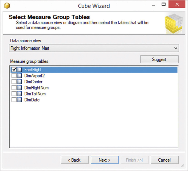
Figure 15.21 Select measure group tables in the cube wizard.
The measure group table is the fact table in the information mart that provides the facts and their measures. You should avoid selecting multiple fact tables here. Instead of doing so, create a new virtual fact table and (if required) another bridge table with the corresponding grain to improve the reusability of business logic that is responsible for defining the right grain in the bridge table and how it is presented to the business user (the virtual fact entity in the information mart).
Select the fact table and click the next button. The next page allows you to select the measures from the source table that should be included in the cube (Figure 15.22).

Figure 15.22 Select measures for the cube.
In this example, the following measures should be included in the flight cube:
• Dep Delay
• Dep Delay Minutes
• Taxi Out
• Taxi In
• Arr Delay
• Arr Delay Minutes
• CRS Elapsed Time
• Actual Elapsed Time
• Air Time
• Flights
• Distance
• Carrier Delay
• Weather Delay
• NAS Delay
• Security Delay
• Late Aircraft Delay
• Fact Flight Count
Select the above measures and click the next button. The next page is shown in Figure 15.23.

Figure 15.23 Select existing dimensions to be included in the cube.
The page presented in Figure 15.23 allows you to include existing dimensions, which have been created in section 15.2. Select all required dimensions and select the next button to add additional dimensions (Figure 15.24).

Figure 15.24 Select new dimensions to be included in the cube.
If the fact table includes dimensional attributes which are not provided as dimension tables in the information mart, the dimensions can be set up using this page. Because there are no additional dimensions to be created in the FactFlight table, click the next button to continue. The next page, shown in Figure 15.25, presents the configuration of the cube for reviewing.

Figure 15.25 Completing the cube wizard.
Review the cube configuration presented on the page and provide a meaningful cube name for the business user. Select the finish button to complete and close the cube wizard. The cube is put into design mode and the logical model of the cube should be shown (Figure 15.26).

Figure 15.26 Logical model of the flight cube.
The model should include the fact table FactFlight and all selected dimension tables. Review the logical model before starting the cube processing and deployment that is required for using it in the front-end tool of your choice.
Note that the logical model for the cube, presented in Figure 15.26, provides only a simplified cube for flight information. There are many dimensions and measures missing from the cube that are required to put this cube into production. However, it serves as an appropriate final example for the information mart created in this book.
15.3.1. Processing the Cube
Once the cube has been defined, it needs to be processed and deployed to the Analysis Services database on the database back-end. To process the cube, open the context menu of the cube in the solution explorer and select process. Make sure that the cube definition is saved. The dialog shown in Figure 15.27 appears on the screen.

Figure 15.27 Process flight information mart cube.
Click the run button in the dialog to initiate the cube processing. The next dialog, presented in Figure 15.28, shows the progress of the cube processing.

Figure 15.28 Process progress.
Wait until the cube processing completes and close the dialog using the close button. The cube is now ready for use.
15.4. Accessing the Cube
To retrieve aggregated information from the cube, open Microsoft SQL Server Management Studio, connect to the Analysis Services database and create a new MDX query on the database just created. Enter the following MDX statement:

This statement returns the distance flown in October 2003 by carrier. It is only one way of retrieving information from the cube, giving end-users full freedom to choose the measures and dimensions provided by the cube for ad-hoc access.
..................Content has been hidden....................
You can't read the all page of ebook, please click here login for view all page.