Chapter 11

Fuzzy In Equals Fuzzy Out: Pushing Imprecision through a Formula

In This Chapter

Checking out the general concept of error propagation

Propagating errors through simple mathematical expressions

Getting a grip on error propagation for more complicated expressions

In Chapters 9 and 10, I describe how you can estimate the precision of anything you can measure (like height and weight) or count (such as hospital admissions, adverse events, and responses to treatment). In this chapter, I show you how to estimate the precision of things you calculate from the things you measure or count (for example, you can calculate body mass index from height and weight measurements). I explain the concept of error propagation, and I describe some simple rules you can use for simple expressions, such as those involving only addition, subtraction, multiplication, and division. Then I show you how to deal with simple or complicated expressions without having to do any calculations at all, using readily available software to do all the hard work for you.

Knowing how to make these calculations is important because often you can’t directly measure the thing you’re really interested in; you have to calculate it from one or more other things that you can measure. You have to be able to determine the precision of these calculated numbers as well, because any number whose accuracy or precision is completely unknown is completely worthless.

Note: For the purposes of this chapter, it doesn’t matter whether you choose to express precision as a standard error (SE) or as a margin of error (the distance from the number to the ends of a confidence interval, as I describe in Chapter 10). I refer to SE throughout this chapter, but the techniques I describe work for margin of error as well.

Understanding the Concept of Error Propagation

A less extreme form of the old saying “garbage in equals garbage out” is “fuzzy in equals fuzzy out.” Random fluctuations in one or more measured variables produce random fluctuations in anything you calculate from those variables. This process is called the propagation of errors. You need to know how measurement errors propagate through a calculation that you perform on a measured quantity.

Here’s a simple way to estimate the SE of a variable (Y) that’s calculated from almost any mathematical expression that involves a single variable (X). Starting with the observed X value (which I call Xo), and its standard error (SE), just do the following 3-step calculation:

1. Evaluate the expression, substituting the value of Xo – SE for X in the formula. Call the result Y1.

2. Evaluate the expression, substituting the value of Xo + SE for X in the formula. Call the result Y2.

3. The SE of Y is simply (Y2 – Y1)/2.

Here’s an example that shows how (and why) this process works.

Suppose you measure the diameter (d) of a coin as 2.3 centimeters, using a caliper or ruler that you know (from past experience) has an SE of ±0.2 centimeters. Now say that you want to calculate the area (A) of the coin from the measured diameter. If you know that the area of a circle is given by the formula A = (π/4)d2, you can immediately calculate the area of the coin as (π/4)2.32, which you can work out on your calculator to get 4.15475628 square centimeters. Of course, you’d never report the area to that many digits because you didn’t measure the diameter very precisely. So just how precise is your calculated area? In other words, how does that ±0.2-centimeter SE of d propagate through the formula A = (π/4)d2 to give the SE of A?

One way to answer this question would be to consider an interval of uncertainty around the observed diameter (d) that goes from one SE below d to one SE above d. Interval of uncertainty isn’t an official statistical term, but it has a great abbreviation (IOU), so I use it in this section. The IOU, as I’ve just defined it, is always two SEs wide. In the coin example, the diameter’s IOU extends from 2.3 – 0.2 to 2.3 + 0.2, or from 2.1 to 2.5 centimeters.

Now figure out the areas corresponding to the diameters at the lower and upper ends of the IOU. Using 2.1 for d in the area formula gives A = 3.46, and using 2.5 for d gives A = 4.91. So the IOU for the area of the coin goes from 3.46 to 4.91 square centimeters. The width of this IOU is 4.91 – 3.46, or 1.45 square centimeters, which represents two SEs for the area. So the SE of the area is 1.45/2, or 0.725 square centimeter.

These calculations are illustrated in Figure 11-1. The curved line represents the formula A = (π/4) × d2. The dark arrows show how the measured diameter (2.3 centimeters), when plugged into the formula, produces a calculated area of about 4.15 square centimeters. The lighter colored gray arrows represent the lower and upper ends of the IOU and show how the IOU for the diameter produces an IOU for the area.

Illustration by Wiley, Composition Services Graphics

Figure 11-1: How uncertainty in diameter becomes uncertainty in area.

The SE of the area depends on the SE of the diameter and the slope of the curve. In fact, the SE of the area is equal to the SE of the diameter multiplied by the slope of the curve. I express this relationship as a formula later in this chapter.

Unfortunately, the simple procedure illustrated in this example can’t be generalized to handle functions of two or more variables, such as calculating a person’s body mass index from height and weight. Mathematicians have derived a very general formula for calculating (approximately) how SEs in one or more variables propagate through any expression involving those variables, but it’s very complicated, and to use it you have to be really good at calculus or you’ll almost certainly make mistakes along the way.

Fortunately, there are much better alternatives, all of which I cover in the rest of this chapter:

You can use some simple error-propagation formulas for simple expressions.

Even easier, you can go to a web page that does the error-propagation calculations for functions of one or two variables.

You can use a very general simulation approach that can easily analyze how errors propagate through even the most complicated expressions, involving any number of variables.

Using Simple Error Propagation Formulas for Simple Expressions

Even though some general error-propagation formulas are very complicated (as I note in the preceding section), the rules for propagating SEs through some simple mathematical expressions are much easier to work with. Here are some of the most common simple rules.

All the rules that involve two or more variables assume that those variables have been measured independently; they shouldn’t be applied when the two variables have been calculated from the same raw data.

Adding or subtracting a constant doesn’t change the SE

Adding (or subtracting) an exactly known numerical constant (that has no SE at all) doesn’t affect the SE of a number. So if x = 38 ± 2, then x + 100 = 138 ± 2. Likewise, if x = 38 ± 2, then x – 15 = 23 ± 2.

Multiplying (or dividing) by a constant multiplies (or divides) the SE by the same amount

Multiplying a number by an exactly known constant multiplies the SE by that same constant. This situation arises when converting units of measure. For example, to convert a length from meters to centimeters, you multiply by exactly 100, so a length of an exercise track that’s measured as 150 ± 1 meters can also be expressed as 15,000 ± 100 centimeters.

For sums and differences: Add the squares of SEs together

When adding or subtracting two independently measured numbers, you square each SE, then add the squares, and then take the square root of the sum, like this:

For example, if each of two measurements has an SE of ±1, and those numbers are added together (or subtracted), the resulting sum (or difference) has an SE of , which is or about ±1.4.

A useful rule to remember is that the SE of the sum or difference of two equally precise numbers is about 40 percent larger than the SE of one of the numbers.

When two numbers of different precision are combined (added or subtracted), the precision of the result is determined mainly by the less precise number (the one with the larger SE). If one number has an SE of ±1 and another has an SE of ±5, the SE of the sum or difference of these two numbers is , which is , which is 5.1, or only slightly larger than the larger of the two individual SEs.

For averages: The square root law takes over

The SE of the average of N equally precise numbers is equal to the SE of the individual numbers divided by the square root of N.

For example, if your lab analyzer can determine a blood glucose value with an SE of ±5 milligrams per deciliter (mg/dL), then if you split up a blood sample into four specimens, run them through the analyzer, and average the four results, the average will have an SE of , or ±2.5 mg/dL. The average of four numbers is twice as precise as (has one-half the SE of) each individual number.

For products and ratios: Squares of relative SEs are added together

The rule for products and ratios is similar to the rule for adding or subtracting two numbers that I describe earlier in this chapter, except that you have to work with the relative SE instead of the SE itself. The relative SE of x is the SE of x divided by the value of x. So, a measured weight of 50 kilograms with an SE of 2 kilograms has a relative SE of 2/50, which is 0.04 or 4 percent. When multiplying or dividing two numbers, square the relative standard errors, add the squares together, and then take the square root of the sum. This gives you the relative SE of the product (or ratio). The formulas are

This formula may look complicated, but it’s actually very easy to use if you work with percent errors (relative precision). Then it works just like the “add the squares” rule for addition and subtraction. So if one number is known to have a relative precision of ± 2 percent, and another number has a relative precision of ± 3 percent, the product or ratio of these two numbers has a relative precision (in percentage) of , which is or ±3.6 percent.

Note that multiplying a number by an exactly known constant doesn’t change the relative SE. For example, doubling a number represented by x would double its SE, but the relative error (SE/x) would remain the same because both the numerator and the denominator would be doubled.

For powers and roots: Multiply the relative SE by the power

For powers and roots, you have to work with relative SEs. When x is raised to any power k, the relative SE of x is multiplied by k; and when taking the kth root of a number, the SE is divided by k. So squaring a number doubles its relative SE, and taking the square root of a number cuts the relative SE in half.

For example, because the area of a circle is proportional to the square of its diameter, if you know the diameter with a relative precision of ±5 percent, you know the area with a relative precision of ±10 percent.

Take another look at the example from the beginning of this chapter. The diameter of the coin is 2.3 ± 0.2 centimeters, for a relative precision of 0.2/2.3 = 0.087, or an 8.7 percent relative SE. And the area of the circle is calculated as 4.155 ± 0.725 square centimeters for a relative precision of 0.725/4.155 = 0.1745, or a 17.45 percent relative SE, which is almost exactly twice the relative SE of the diameter. Notice that the constant (π/4) is completely ignored because relative errors aren’t affected by multiplying or dividing by a known constant.

If k is negative (such as x–2, which is 1/x2), you ignore the minus sign and use the absolute value of k. So the relative SE of 1/x2 is twice the relative SE of x. A special case of this rule is the simple reciprocal: The relative SE of 1/x is equal to the relative SE of x. In other words, if x is precise to ±1 percent, then 1/x is also precise to ±1 percent.

For example, under certain assumptions, the half-life (t1/2) of a drug in the body is related to the terminal elimination rate constant (ke) for the drug by the formula: t1/2 = 0.693/ke. A pharmacokinetic regression analysis (see Chapter 21) might produce the result that ke = 0.1633 ± 0.01644 (ke has units of “per hour”). You can calculate that t1/2 = 0.693/0.1633 = 4.244 hours. How precise is this half-life value? First you calculate the relative SE of the ke value as SE(ke )/ke, which is 0.01644/0.1633 = 0.1007, or about 10 percent. Because ke has a relative precision of ± 10 percent, t1/2 also has a relative precision of ± 10 percent, because t1/2 is proportional to the reciprocal of ke (you can ignore the 0.693 entirely, because relative errors are not affected by multiplying or dividing by a known constant). If the t1/2 value of 4.244 hours has a relative precision of 10 percent, then the SE of t1/2 must be 0.4244 hours, and you report the half-life as 4.24 ± 0.42 hours.

Handling More Complicated Expressions

Sometimes you have an expression that can’t be handled by the simple rules described earlier in this chapter. The expression may be a very complicated expression and may involve logarithms, exponentials, or trigonometric functions. In these situations, you still have some options, as you find out in the following sections.

Using the simple rules consecutively

A complicated expression can often be broken down into a sequence of simple operations, which can then be analyzed by the rules described earlier in this chapter. For example, you can calculate the SE of the result of xy + z from the SEs of x, y, and z by first using the product rule to get the SE of xy. Then you can use the addition rule with the SE of xy and the SE of z to get the SE of xy + z. But you have to be very careful going back and forth between SEs and relative SEs because you’re likely to make a mistake somewhere in the calculations. It’s much easier (and safer) to have the computer do all the calculations for you. Keep reading!

Checking out an online calculator

The web page at statpages.info/erpropgt.html calculates how precision propagates through almost any expression involving one or two variables. It even handles the case of two variables with correlated fluctuations. You simply enter the following items:

The expression, using a fairly standard algebraic syntax (JavaScript)

The values of the variable or variables

The corresponding SEs

The web page then evaluates the general error-propagation formulas and shows you the value of the resulting number, along with its SE. Figure 11-2 shows how the web page handles the simple coin-area example I use in the earlier section Understanding the Concept of Error Propagation.

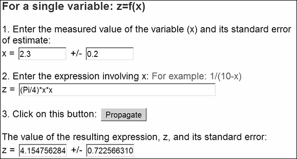
Screenshot courtesy of John C. Pezzullo, PhD

Figure 11-2: Using the web page to calculate error propagation through an expression with one variable.

The expression must refer to the variable (diameter) as x, and the squaring of x must be indicated as x * x, because JavaScript doesn’t allow x2. The web page knows what the value of pi is. It calculates an area of 4.15 square centimeters and an SE of 0.72 square centimeter, in good agreement with the calculations I describe earlier.

The web page can also analyze error propagation through expressions involving two measured values. Suppose you want to calculate body mass index (BMI, in kilograms per square meter) from a measured value of height (in centimeters) and weight (in kilograms), using the formula: BMI = 10,000weight/height2. Suppose the measured height is 175 ± 1 centimeter, and the weight is 77 ± 1 kilograms (where the ± numbers are the SEs). The BMI is easily calculated as 10,000 × 77/1752, or 25.143 kg/m2. But what’s the SE of that BMI? Figure 11-3 shows how the web page performs that calculation.

Screenshot courtesy of John C. Pezzullo, PhD

Figure 11-3: Using the web page to calculate error propagation through an expression with two variables.

The page requires that height and weight be called x and y, respectively. I entered the square of the height as (x * x), because JavaScript doesn’t allow x2. I entered 0 for the error-correlation term because height and weight are two independent measurements (using different instruments). The resulting BMI produced by the web page was 25.1 ± 0.4 kilograms per square meter.

Simulating error propagation — easy, accurate, and versatile

Finally, I briefly describe what is probably the most general error-propagation technique (also called Monte-Carlo analysis). You can use this technique to solve many difficult statistical problems. Calculating how SEs propagate through a formula for y as a function of x works like this:

1. Generate a random number from a normal distribution whose mean equals the value of x and whose standard deviation is the SE of x.

2. Plug the x value into the formula and save the resulting y value.

3. Repeat this step a large number of times.

The resulting set of y values will be your simulated sampling distribution for y.

4. Calculate the SD of the y values.

The SD of the simulated y values is your estimate of the SE of y. (Remember, the SE of a number is the SD of the sampling distribution for that number.)

You can perform these calculations very easily using the free program Statistics 101 (see Chapter 4). With very little extra effort, this software can give you the confidence interval and even a histogram of the simulated areas. And simulation can easily and accurately handle non-normally distributed measurement errors. For the coin-area example, the program (only four lines long) generates the output shown in Figure 11-4. The SE of the coin area from this simulation is about 0.72, in good agreement with the value obtained by the other methods I describe earlier in this chapter.

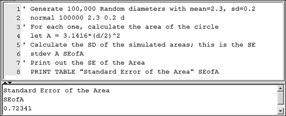
Screenshot courtesy of John C. Pezzullo, PhD

Figure 11-4: Using Statistics 101 to simulate error propagation.