A P P E N D I X  B

SQL Practical Introduction

Structured Query Language (SQL) is the most widely used language to interact with DBMSs. The purpose of this appendix is not to provide a comprehensive manual of SQL but rather to list and explain the most common concepts, terms, and statements. Most DBMSs don’t support the whole SQL standard. Moreover, vendors sometimes add nonstandard elements that, in practice, prevent full portability across DBMSs. In this appendix, I’ll limit myself to standard elements. To help you identify nonstandard keywords, I have included Table B-12 at the end of this appendix, which lists the standard keywords that should work with most implementations.

SQL Terminology

Data is organized in tables consisting of rows and columns. This is a natural way of organizing data, and you’re probably familiar with it through the use of spreadsheets. Nevertheless, although there are some similarities, a database table is not an Excel worksheet. For example, in a spreadsheet, you can assign data types to individual cells, while in a database, all the cells of a column have the same data type. The column definitions, each with their name and the type of data permitted, are the core of the table structure.

For example, a table of employees would probably include columns named FirstName, LastName, and SocialSecurityNumber containing strings of text; columns named EmployeeNumber and YearSalary would contain numbers; and columns named DateOfBirth and EmployedSince would contain dates. The data associated with each employee would then all be stored into a row.

A field is an individual data item within a table, corresponding to the intersection of a row and a column. This would be a cell in a spreadsheet.

One or more columns can be specified as unique keys, used to identify each individual employee. For this purpose, you could use either one of the columns mentioned previously (e.g., EmployeeNumber), or the combination of first and last name. The unique key used in preference over the others is called the primary key of a table.

An additional type of key is the foreign key. In this case, the column is defined as a reference to a unique key of another table. Besides avoiding duplication of data, this type of constraint increases the consistency of the database. For example, a table containing customer contracts could include a column referring to the column of employee numbers defined in the employee table. This would ensure that each contract would be associated with an existing salesperson.

The DBMS can build an index for each key, so that the data can be retrieved more quickly. This will obviously slow down insertion and deletion of rows (i.e., of new records), because the DBMS will have to spend time updating the indexes, but most databases are more frequently interrogated than modified. Therefore, it usually pays to define indexes, at least those that can speed up the most common queries. Here you have a hint of another difference from Excel: in a database table, the data items are not moved around once they’re inserted; if you want to access them in a particular order, you must either sort them every time or create an index. You will learn about indexing later in this appendix.

Sometimes it’s useful to present only some columns and rows, as if they were a table in their own right. Such virtual tables are called views. Under certain circumstances (I’ll discuss this further when I describe individual statements, later in this chapter), you can also use views to collect columns from different tables and handle them as if they belonged to a single table.

Transactions

Transactions deserve a little more attention, because they represent a key concept in DBMSs. A transaction indicates a series of database operations that have to be performed without interruption—that is, without any other operation “sneaking in” between them. To make sense of this, you have to think in terms of concurrent access to the same tables.

For example, imagine the following scenario, in which two money transfers involve three bank accounts:

1. Transfer $100 from account A to account B
2. Transfer $200 from account B to account C

Conceptually, each transfer consists of the following operations:

• Read the balance of the source account.
• Reduce it by the amount of the transfer.
• Write it back.
• Read the balance of the destination account.
• Increase it by the amount of the transfer.
• Write it back.

Now, imagine that transfer number 2 starts while transfer number 1 is not yet completely done, as illustrated in the sequence of elementary operations listed in Table B-1.

The owner of account B is going to be very happy, because she will end up with $200 more than what she actually owns. The problem is that the two steps numbered 6 and 11 should have not been executed in that order. Let’s say that account B initially held $500. At the end, it should hold $500 + $100 - $200 = $400, but this is not what happened. Just before the end of the first transfer, when the balance of $600 was about to be written back, the second transfer started. The balance of account B stored in the database was changed as a result of the second transfer, but when the first transfer resumed and completed, the balance of $600 was written back to account B. The effect of the second transfer was “forgotten.” As far as account B was concerned, it was as if the second transfer hadn’t happened!

You can solve this problem by handling each transfer as a transaction. The second transfer won’t start until the first one is completed, and by then, the balance of account B will have been updated to reflect the first transfer.

A transaction is characterized by four properties—atomicity, consistency, isolation, and durability (ACID):

• Atomicity: It guarantees that either all the individual steps of an operation are performed or none at all. You must not be able to perform partial transactions.
• Consistency: It refers to the fact that a transaction is not supposed to violate the integrity of a database. For example, it shouldn’t be able to store a negative value in a numeric field that is supposed to be positive. When it comes to distributed systems, it also means that all the nodes will have consistent values.
• Isolation: It means that concurrent operations cannot see intermediate values of a transaction. Lack of isolation is what caused the example of Table B-1 to fail, when the balance of account B could be read even though the transaction that was modifying it was not yet complete. Unfortunately, the serialization of the transactions (i.e., performing them one after the other) has an impact on performance precisely when there is a high workload. Lack of isolation is a problem in the example, but this is not always the case. For example, it might not matter that searches on a list of products take place while products are being added or removed. Given the potential impact on performance, you might decide in some cases to ignore the existence of concurrent transactions.
• Durability: It refers to the capacity of a DBMS to guarantee that a transaction, once completed, is never going to be “forgotten,” even after a system failure.

Conventions

I’ll use the following conventions to describe SQL statements:

• SQL keywords that you must enter exactly as shown are in uppercase (e.g., CREATE). Note that most keywords can actually be in lowercase.
• Variable values are in lowercase (e.g., db_name).
• Elements that you can omit are enclosed in square brackets (e.g., [WITH]).
• References to further definitions are enclosed in angle brackets (e.g., <create_spec>).
• The ellipsis immediately preceding a closing square bracket means that you can repeat the element enclosed between the brackets (e.g., [<create_spec> ...]). That is, you can omit the element, enter it once, or enter it more than once.
• Mutually exclusive alternatives are enclosed in curly brackets and separated by vertical bars (e.g., {DATABASE | SCHEMA}). You must enter one (and only one) of them.
• I close every statement with a semicolon, although, strictly speaking, it is not part of the official syntax. I do so because it makes for easier reading and reminds you that you must type the semicolon when including the statement in scripts.

For example, Listing B-1 shows part of the SQL statement used to create a database. It begins with the CREATE keyword followed by either DATABASE or SCHEMA and a database name. It is then possible (but not mandatory) to add one or more <create_spec> elements, the meaning of which is defined separately.

Statements

In general, regardless of whether we’re talking about database organization, table structure, or actual data, you’ll need to perform four basic operations: create, retrieve, update, and delete (CRUD). The corresponding SQL statements begin with a keyword that identifies the operation (e.g., INSERT, SELECT, UPDATE, or DELETE), followed when necessary by a keyword specifying on what type of entity the operation is to be performed (e.g., DATABASE, TABLE, or INDEX) and by additional elements. You use the SELECT statement for retrieving information.

You can create databases, tables, and indexes with the CREATE statement, update them with ALTER, and delete them with DROP. Similarly, you can create and delete views with CREATE and DROP, but you cannot update them once you’ve created them. You use INSERT to create new rows within a table, and you use DELETE to delete them. The UPDATE statement lets you modify entire rows or one or more individual fields within them.

The statements that let you modify the structures are collectively referred to as Data Definition Language (DDL), while those that let you modify the content are called Data Manipulation Language (DML).

That said, you won’t find anything about ALTER DATABASE and ALTER INDEX in this appendix, because there is very little you can update in a database or an index definition once you’ve created them, and there is no agreement among DBMS vendors about what you can do. Table B-2 shows a summary of the possible combinations of keywords. In the following sections, I will explain how to use them going through Table B-2 by columns. This will tell you how to create new structures and new data, how to modify them, and how to remove them.

In many applications, the structure of databases, tables, indexes, and views, once initially defined, remains unchanged. Therefore, you’ll often need within your applications only the statements operating on rows and fields. In any case, you’ll certainly need SELECT, which you use to interrogate databases both in terms of their structure and the data they contain. Finally, to complete the list of statements you’re likely to need when developing applications, I’ll also describe START TRANSACTION, COMMIT, and ROLLBACK, which you need to use transactions.

SQL interprets all text enclosed between /* and */ as comments and ignores it.

The WHERE Condition

When you want to retrieve, update, or delete rows, you obviously have to identify them. You do this with the WHERE keyword followed by a <where_condition>. Listing B-2 shows you the format of this condition. I explain WHERE before discussing individual statements, because you’ll need it for several of them.

Note that the WHERE condition is more powerful (and complex) than what I explain here. You could actually include complete query statements within a condition and use the result of a first search to delimit the scope of the following one. However, to explain such techniques involving subqueries would go beyond the scope of this manual.

I’ll describe the listed possibilities by simply showing and explaining valid examples of WHERE selections on a hypothetical employee table:

• lastname = 'Smith' selects all employees with the family name Smith.
• startdate < '2000-01-01' selects all employees who joined the company before the beginning of the century.
• startdate BETWEEN '2010-01-01' AND '2010-12-31' selects all employees who joined the company in 2010, while startdate NOT BETWEEN '2010-01-01' AND '2010-12-31' selects those who didn’t.
• lastname LIKE 'S%' selects all employees whose family name starts with S. In other words, the percent sign is the SQL equivalent of the asterisk you use when listing a directory from the command line. You can use more than one percent sign in a condition. For example, lastname LIKE 'S%z%a' selects all names that start with S, end with a, and have a z somewhere in between. While the percent sign stands for any number of characters (including none), the underscore stands for exactly one character, like the question mark when listing directories. For example, lastname NOT LIKE '_' selects all names that contain at least two characters (or none, if you allow it when designing the database). The ESCAPE keyword lets you search for strings containing one of the escape characters. For example, lastname LIKE '%!%%' ESCAPE '!' selects all names that contain a percent sign in any position.
• firstname IN ('John', 'Jack') selects all employees who have either John or Jack as their first name.
• middlename IS NULL selects all employees who have no middle name.
• lastname CONTAINING 'qu' selects all employees who have the string “qu” in their family name. This is identical to lastname LIKE '%qu%'.
• lastname STARTING WITH 'Sm' selects all employees whose family name starts with “Sm”. This is identical to lastname LIKE 'Sm%'.
• You can use the logical operators NOT, AND, and OR to build complex conditions. For example, startdate >= '2010-01-01' AND startdate <= '2010-12-31' is equivalent to startdate BETWEEN '2010-01-01' AND '2010-12-31'. To avoid ambiguities, use the parentheses to set the order of execution. For example, lastname CONTAINING 's' OR (lastname CONTAINING 'q' AND lastname NOT CONTAINING 'qu') selects all employees whose family names contain an ‘s’ or a ‘q’, but only if the ‘q’ is not followed by a ‘u’. The statement (lastname CONTAINING 's' OR lastname CONTAINING 'q') AND lastname NOT CONTAINING 'qu' would not select names containing both ‘s’ and “qu”. A name such as “quasi” would be selected by the first condition but not by the second one.

Data Types

When designing your database, you have to decide what type of data you need to store in the columns of your tables. SQL supports different data types to store numbers, text, date/time, and unspecified data (called LOB, for large object), as summarized in Listing B-3.

Numbers

The space reserved in memory for the numeric data types determines their precision—that is, the number of digits they can have. Java and JSP specify the space allocated for each data type, so that they are the same regardless of operating systems and virtual machines. Unfortunately, the same cannot be said of SQL, where the precision of the data types, like so many other things, is vendor-dependent. Therefore, you always have to refer to the manual of your DBMS if you want to be sure that your applications will work correctly. Listing B-4 shows how you specify a numeric data type.

The types DECIMAL (which can be abbreviated to DEC) and NUMERIC require you to specify the total number of digits and the number of decimal places. For example, you specify numbers of the type xxxx as (4), numbers of the type xxx.y as (4,1), and numbers of the type 0.yyy as (3,3). The scale must never exceed the precision. As different DBMS vendors set different defaults, you should always at least specify the precision. When doing so, keep in mind that 18 decimal digits require 64 bits. Therefore, larger precisions might not be accepted by all DBMSs.

The difference between DECIMAL and NUMERIC is that with DECIMAL, the DBMS is free to allocate more space than the minimum required in order to optimize access speed, while with NUMERIC, the number of digits allocated is exactly what you specify as precision.

The other types are easier to use but require some attention, because, again, different DBMS vendors allocate different numbers of bytes for the different data types. If you don’t pay attention, you’ll risk writing code that won’t be portable.

SMALLINT, INTEGER or INT, and BIGINT refer to integer types of different sizes, while the remaining three types refer to numbers with a decimal point. Table B-3 shows the ranges possible with different numbers of bits, and their corresponding data types in Java.

Some versions of MySQL also support the numeric data types BIT and TINYINT, but they are not always supported by other SQL implementations or by all versions of MySQL. I suggest that you stick to the standard types.

Table B-4 lists the number of bits allocated by some vendors to the different SQL data types. I include this information here to help you in case you need to port your code to SQL implementations other than MySQL.

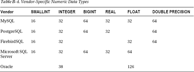
FirebirdSQL supports 64-bit integers, but it doesn’t recognize the type BIGINT. You have to use INT64. Microsoft SQL Server and Oracle aren’t open source DBMSs, but given their large customer bases, I thought you might be interested to know.

Date and Time

Listing B-5 shows how dates and times are defined in SQL, but its simplicity is somewhat misleading, because the DBMSs of different vendors, by now certainly unsurprisingly, behave differently.

One area where the vendors don’t agree is the range of dates. MySQL accepts dates between the year 1000 CE and the year 9999 CE, PostgreSQL between 4713 BCE and 5874897 CE, and FirebirdSQL between 100 CE and February 32767 CE. The bottom line is that any date within our lifetimes should be accepted by every DBMS!

You can use DATE when you’re not interested in the time of the day. It occupies 4 bytes. TIME stores the time of the day in milliseconds and occupies 8 bytes. TIMESTAMP manages to fit both the date and the time of the day in milliseconds into 8 bytes.

You can set date and time values in different formats, but I recommend that you conform to the ISO 8601 standard and set dates as 'YYYY-MM-DD', times as 'HH:MM', 'HH:MM:SS', or 'HH:MM:SS.mmm', and timestamps as a standard date followed by a space and a standard time, as in 'YYYY-MM-DD HH:MM:SS.mmm'. In particular, pay attention to years specified with only two digits, because the different DBMSs interpret the dates differently. MySQL has defined the DATETIME type, but I see no reason for you do adopt it, because MySQL also accepts the standard TIMESTAMP. I mention it here only because you’ll probably encounter it sooner or later.

Text

Listing B-6 shows how you specify strings of characters.

There are only two data types for text: CHARACTER and VARCHAR. CHAR is a synonym of CHARACTER, and CHARACTER VARYING is a synonym of VARCHAR. Use CHARACTER or CHAR to store strings of fixed length, and VARCHAR or CHARACTER VARYING for strings of variable length.

For example, a field of type CHARACTER (16) always occupies 16 bytes. If you use it to store a string of only 6 characters, it will be left-justified and right-padded with 10 spaces. If you attempt to store a string of 19 characters, you’ll only succeed if the last 3 characters are spaces, in which case the DBMS will remove them. Different DBMSs set different limits to the maximum number of characters you can store into a CHARACTER data type, but they will all accept 255 characters. If you need more than that, check the user manual of the DBMS you’re using.

The practical difference between VARCHAR and CHARACTER is that with VARCHAR, the DBMS stores the strings as they are, without padding. Also, with VARCHAR, you should be able to store up to 32,767 characters with all DBMSs.

Large Objects

LOBs let you store large amount of data, including binary data. This is an alternative to saving data in files and then storing their URIs into the database. In general, I am reluctant to store in a database large blocks of data that can be stored in the file system outside the database: like images, video clips, documents, and executable code. By storing data outside the database, you can easily access it with other tools, but by doing so, you also risk compromising the integrity of the data and leave references in the database that point to nonexisting files.

We have to distinguish between binary large objects (BLOBs) and character large objects (CLOBs). Unfortunately, once more, the major DBMS vendors haven’t agreed. See Listing B-7 for the generalized definition of LOBs.

LOBs can store up to 64KB of data. MEDIUMBLOBs can store up to 16MB and LONGBLOBs up to 4GB. Once more, check the user manual of your DBMS if you are not sure.

SELECT

SELECT retrieves data from one or more tables and views. See Listing B-8 for a description of its format.

In part, the complication of SELECT is due to the fact that you can use it in two ways: to retrieve actual data or to obtain the result of applying a function to the data. To make it worse, some of the elements only apply to one of the two ways of using SELECT. To explain how SELECT works, I’ll split the two modes of operation.

SELECT to Obtain Data

Listing B-9 shows how you use SELECT to obtain data.

Conceptually, it is simple: SELECT one, some, or all columns FROM one or more tables or views WHERE certain conditions are satisfied; then present the rows ORDERed as specified. Some examples will clarify the details:

• SELECT * is the simplest possible SELECT, but you’ll probably never use it. It returns everything you have in your database.
• SELECT * FROM table is the simplest practical form of SELECT. It returns all the data in the table you specify. The DBMS returns the rows in the order it finds most convenient, which is basically meaningless to you and me. Instead of a single table, you can specify a mix of tables and views separated by commas.
• SELECT a_col_name, another_col_name FROM table still returns all the rows of a table, but for each row, it returns only the values in the columns you specify. Use the keyword DISTINCT to tell the DBMS that it should not return any duplicate row. The default is ALL. You can also use column positions instead of column names.
• SELECT * FROM table WHERE condition only returns the rows for which the condition you specify is satisfied. Most SELECTs include a WHERE condition. Often only a single row is selected—for example, when the condition requires a unique key to have a particular value.
• SELECT * FROM table ORDER BY col_name returns all the rows of a table ordered on the basis of a column you specify. Note that you can provide more than one ordering. For example, SELECT * FROM employee_tbl ORDER BY last_name, first_name returns a list of all employees in alphabetical order. With the keyword DESD, you specify descending orderings.
• SELECT * FROM table LIMIT first, count returns count rows starting from first. You can obtain the same result with SELECT * FROM table LIMIT count OFFSET first. Be warned that not all DBMSs support both formats. I discourage you to use this element, because it doesn’t deliver entirely predictable results. I only include it here because you could find it useful to debug some database problem.

SELECT to Apply a Function

Sometimes you need to obtain some global information on your data and are not interested in the details. This is where the second format of SELECT comes to the rescue. Listing B-10 shows how you use SELECT to apply a function.

Here are some examples of how you apply a function with SELECT:

• SELECT COUNT (*) FROM employee_tbl counts the number of rows in the employee table.
• SELECT department, citizenship, gender COUNT(employee_id) FROM employee_tbl GROUP BY department, citizenship, gender provides counts of employees for each possible department, citizenship, and gender combination. If you append WITH ROLLUP to the statement, you’ll also obtain partial totals, as shown in the example presented in Table B-5.
• SELECT last_name COUNT(first_name) FROM employee_tbl GROUP BY first_name HAVING COUNT(first_name) > 1 counts the number of first names for each family name but only reports the family names that appear with more than one first name. HAVING has the same function for the aggregated values produced by GROUP BY that WHERE had for data selection.

JOINs

When describing SQL terminology, I said that a foreign key is a reference to a unique key of another table. This means that information associated with each unique value of that key can be in either table or in both tables. For example, in a database representing a bookstore, you could imagine having one table with book authors and one with books. The name of the author would be a unique key in the authors’ table and would appear as a foreign key in the books’ table. Table B-6 shows an example of the authors’ table.

Table B-7 shows the books’ table.

If you perform the query SELECT * FROM books, authors;, the DBMS will return 15 combined rows, the first 7 of which are shown in Table B-8.

In other words, all books would be paired with all authors. This doesn’t look very useful.

You can get a more useful result when you perform the following query:

Table B-9 shows its result.

You can achieve the same result with the JOIN keyword:

The result is the same, but conceptually, the JOIN syntax is clearer, because it states explicitly that you want to join two tables matching the values in two columns.

There is another type of JOIN, called OUTER JOIN, which also selects rows that appear in one of the two tables. For example, the following two SELECTs return the results shown respectively in Tables B-10 and B-11:

while this line of code returns the result shown in Table B-11:

To decide of which table you want to include all rows, choose LEFT or RIGHT depending on whether the table name precedes or follows the JOIN keyword in the SELECT statement.

You’d probably like to obtain a list with the names of all authors, regardless of whether they appear only in the first table, only in the second table, or in both tables. Can you have a JOIN that is both LEFT and RIGHT at the same time? The answer is that the SQL standard defines a FULL JOIN, which does exactly what you want, but MySQL doesn’t support it.

CREATE DATABASE

CREATE DATABASE creates a new, empty database. See Listing B-11 for a description of its format.

The DATABASE and SCHEMA keywords are equivalent, and the DEFAULT keyword is only descriptive. The default character set determines how strings are stored in the database, while the collation defines the rules used to compare strings (i.e., precedence among characters).

When using SQL with Java and JSP, you need to specify the Unicode character set, in which each character is stored in a variable number of bytes. With a minimal database creation statement such as CREATE DATABASE 'db_name', you risk getting the US-ASCII character set, which is incompatible with Java. Therefore, always specify Unicode, as in the following statement:

In fact, there are several Unicode character sets, but utf8 is the most widely used and also the most similar to ASCII. As such, it is the best choice for English speakers. You don’t need to bother with specifying any collation. The default will be fine.

CREATE TABLE

CREATE TABLE creates a new table, together with its columns and integrity constraints, in an existing database. See Listing B-12 for a description of its format.

To understand how CREATE TABLE works, concentrate on the first line of Listing B-12. It says that a table definition consists of a table name followed by the definition of one or more columns and possibly some table constraints. In turn, each column definition consists of a column name followed by the definition of a data type, a dimension, a default, and possibly some column constraints.

The following examples and comments should make it clear:

• CREATE TABLE employee_tbl (employee_id INTEGER) creates a table with a single column of type INTEGER and without any constraint. If you want to ensure that the employee ID cannot have duplicates, append the UNIQUE constraint to the column definition: CREATE TABLE employee_tbl (employee_id INTEGER UNIQUE).
• With DEFAULT, you can set the value to be stored in a field when you insert a new row. For example, the column definition employee_dept VARCHAR(64) DEFAULT '' sets the department to an empty string (without the DEFAULT element, the field is set to NULL). The distinction between an empty string and NULL is important when working with Java and JSP, because you can rest assured that a variable containing an unforeseen NULL will sooner or later cause a runtime exception. To avoid setting a field to NULL by mistake, append NOT NULL to a column definition. This will ensure that you get an error when you insert the row and not later when you hit the unexpected NULL. It will make debugging your code easier.
• The column constraints UNIQUE and PRIMARY KEY ensure that the values stored in that column are unique within the table. You can specify the PRIMARY KEY constraint only for one column of each table, while you can specify UNIQUE even for all columns of a table, if that is what you need.
• Use the column constraint REFERENCES to force consistency checks between tables. For example, if you store the list of departments in the table department_tbl, which includes the column dept_name, you could use REFERENCES to ensure that all new employee records will refer to existing departments. To achieve this result, when you create the employee table, define the employee’s department column as follows: employee_dept VARCHAR(64) REFERENCES department_tbl (dept_name). This will make it impossible for the creator of the employee record to enter the name of a nonexisting department. Note that you must have defined the referenced columns with the UNIQUE or PRIMARY KEY constraints, because this constraint actually creates foreign keys. It wouldn’t make sense to reference a column that allows duplicate values, because then you wouldn’t know which row you would actually be referring to.
• The ON DELETE and ON UPDATE elements, which you can append to the REFERENCES column constraint, tell the DBMS what you want to happen when the referenced column (or columns) are deleted or updated. For example, if the department named 'new_product' is merged into 'development' or renamed to 'design', what should happen with the records of employees currently working in 'new_product'? You have four possibilities to choose from. With NO ACTION, you direct the DBMS to leave the employee record as it is. With SET NULL and SET DEFAULT, you choose to replace the name of the updated or deleted department with NULL or the default value, respectively. With CASCADE, you tell the DBMS to repeat for the referencing employee record what has happened with the referenced department record. That is, if the employee_dept column of the employee table has the ON UPDATE CASCADE constraint, you can change the department name in the department table and automatically get the same change in the employee table. Great stuff, but if you have the constraint ON DELETE CASCADE and remove a department from the department table, all the employee records of the employee table referencing that department will disappear. This is not necessarily what you want to happen. Therefore, you should be careful when applying these constraints.
• The CHECK column constraint only lets you create columns that satisfy the specified check condition. For example, to ensure that a bank account can only be opened with a minimum balance of $100, you could define a column named initial_balance with the following constraint: CHECK (initial_balance >= '100.00').
• The table constraints are similar to the column constraints, both in meaning and in syntax. However, there is one case in which you must use the table constraints: when you want to apply the UNIQUE or PRIMARY KEY constraints to a combination of columns rather than to a single one. For example, you might need to require that the combination of first and last name be unique within an employee table. You could achieve this result with the following constraint on the employee table: UNIQUE (last_name, first_name).
• The purpose of CONSTRAINT constraint_name is only to associate a unique name to a constraint. This then allows you to remove the constraint by updating the table with the DROP constraint_name element. As you never know whether you’ll need to remove a constraint in the future, you should play it safe and name the constraints you apply. Otherwise, in order to remove the unnamed constraint, you would have to re-create the table (without the constraint) and then transfer the data from the original constrained table.

CREATE INDEX

CREATE INDEX creates an index for one or more columns in a table. You can use it to improve the speed of data access, in particular when the indexed columns appear in WHERE conditions. See Listing B-13 for a description of its format.

For example, CREATE UNIQUE INDEX empl_x ON employee_tbl (last_name, first_name) creates an index in which each entry refers to a combination of two field values. Attempts to create employee records with an existing combination of first and last name will fail.

CREATE VIEW

CREATE VIEW lets you access data belonging to different tables as if each data item were part of a single table. Only a description of the view is stored in the database, so that no data is physically duplicated or moved. See Listing B-14 for a description of its format.

Here are some examples of CREATE VIEW:

• CREATE VIEW female_employees AS SELECT * FROM employee_tbl WHERE gender = 'female' creates a view with all female employees. The column names of the view are matched one by one with the column names of the table.
• CREATE VIEW female_names (last, first) AS SELECT last_name, first_name FROM employee_tbl WHERE gender = 'female' creates a similar view but only containing the name columns of the employee table rather than its full rows.
• CREATE VIEW phone_list AS SELECT last_name, first_name, dept_telephone, phone_extension FROM employee_tbl, department_tbl WHERE department = dept_no creates a view with columns from both the employee and the department tables. The columns of the view are named like the original columns, but it would have been possible to rename them by specifying a list of columns enclosed in parentheses after the view name. The WHERE condition is used to match the department numbers in the two tables so that the department telephone number can be included in the view. Note that views that join tables are read-only.
• When a view only refers to a single table, you can update the table by operating on the view rather than on the actual table. The WITH CHECK OPTION element prevents you from modifying the table in such a way that you could then no longer retrieve the modified rows. For example, if you create a view WITH CHECK OPTION containing all female employees, it won’t allow you to use the view to enter a male employee or to change the gender of an employee. Obviously, you would still be able to do those operations by updating the employee table directly.

INSERT

INSERT stores one or more rows in an existing table or view. See Listing B-15 for a description of its format.

You can use INSERT to create one row in a table (or a single-table view) from scratch or to create one or more rows by copying data from other tables, as shown in the following examples.

• INSERT INTO employee_tbl (employee_id, first_name, last_name) VALUES ('999', 'Joe', 'Bloke') creates a new row for the employee Joe Bloke. All the columns not listed after the table name are filled with their respective default values. You could omit the list of column names, but the values would be stored beginning from first column in the order in which the columns were created. Be sure that you get the correct order.
• INSERT INTO foreigners SELECT * from employee_tbl WHERE citizenship != 'USA' copies the full records of all employees who are not U.S. citizens to the table foreigners. Note that this is different from creating a view of foreign employees, because the records are actually duplicated and stored in a different table. With a view, you would only specify a different way of accessing the same data. Be extremely cautious when INTO and SELECT refer to the same table. You could create an endless insertion loop. It’s best if you simply refrain from inserting rows by copying the data from rows that are in the same table.

DROP

DROP is the statement you use when you want to remove a database, a table, an index, or a view. See Listing B-16 for a description of their format.

DROP DATABASE removes the database you’re connected to. The rest are pretty self-explanatory. Just one point: with DROP INDEX, you cannot eliminate the indexes that the DBMS automatically creates when you specify the UNIQUE, PRIMARY KEY, or FOREIGN KEY attribute for a column.

DELETE

DELETE removes one or more rows from an existing table or a view that is not read-only. See Listing B-17 for a description of its format.

ALTER TABLE

ALTER TABLE modifies the structure of an existing table. See Listing B-18 for a generalized description of its format.

As you can see from Listing B-18, the DBMS vendors once more cannot agree on how you can modify columns.

The addition or removal of columns and table constraints is pretty straightforward. Refer to CREATE TABLE for a description of <col_def> and <tbl_constr>.

What you can do in terms of changing the definition of an existing column depends on which DBMS you’ve chosen for your application. Only MySQL gives you full flexibility in redefining the column with ALTER TABLE tbl_name CHANGE col_name <col_def>. Note that <col_def> must be complete, including a column name. If you don’t want to change the name of a column, you can use its current name within <col_def>. In fact, besides being compatible with Oracle, the only reason for having MODIFY is that you don’t need to type the same column name twice.

UPDATE

UPDATE modifies the content of one or more existing rows in a table (or single-table view). See Listing B-19 for a description of its format.

For example, use the statement UPDATE employee_tbl SET first_name = 'John' WHERE first_name = 'Jihn' to correct a typing error. Nothing could be simpler.

SET TRANSACTION and START TRANSACTION

The purpose of a transaction is to ensure that nobody else can “sneak in” and modify rows after you’ve read them but before you’ve updated them in the database. The DBMS can achieve this by locking the rows you read within a transaction until you commit your updates. As with other statements, different DBMSs behave differently. Listing B-20 shows what you need to do with MySQL and PostgreSQL, while Listing B-21 shows an example valid for FirebirdSQL.

As you can see, to start a transaction with MySQL and PostgreSQL, you have to execute a SET TRANSACTION and a START, while you only need to execute SET TRANSACTION without START when starting a transaction with FirebirdSQL. Note that all three DBMSs provide additional options, but I’m only showing a mode of operation that is common to them all.

You need to specify the ISOLATION LEVEL if you want to write portable code, because the three DBMSs have different defaults.

COMMIT and ROLLBACK

COMMIT confirms the updates you’ve performed since starting the current transaction and terminates it. ROLLBACK discards the updates and returns the database to its condition prior to the current transaction. Their syntax couldn’t be simpler: COMMIT; and ROLLBACK;.

Reserved SQL Keywords