3.11 Reference posterior distributions

3.11.1 The information provided by an experiment

Bernardo (1979) suggested another way of arriving at a reference standard for Bayesian theory. The starting point for this is that the log-likelihood ratio can be regarded as the information provided by the observation x for discrimination in favour of against (cf. Good, 1950, Section 6.1). This led Kullback and Leibler (1951) to define the mean information in such data to be

(cf. Kullback, 1968, and Barnett, 1999, Section 8.6).1 Note that although there is a relationship between information as defined here and Fisher’s information I as defined in Section 3.3 earlier (see Kullback, 1968, Chapter 2, Section 6), you are best advised to think of this as a quite separate notion. It has in common with Fisher’s information the property that it depends on the distribution of the data rather than on any particular value of it.

Following this, Lindley (1956) defined the expected amount of information that the observation x will provide about an unknown parameter θ when the prior density for θ is to be

The observation x is, of course, random, and hence we can define the expected information that the observation x will provide to be

(a similar expression occurs in Shannon, 1948, Section 24). Two obviously equivalent expressions are

It is easily seen using the usual change-of-variable rule that the information defined by this expression is invariant under a one-to-one transformation. It can be used as a basis for Bayesian design of experiments. It has various appealing properties, notably that with equality if and only if does not depend on θ (see Hardy, Littlewood and Pólya, 1952, Theorem 205). Further, it turns out that if an experiment consists of two observations, then the total information it provides is the information provided by one observation plus the mean amount provided by the second given the first (as shown by Lindley, 1956).

We now define to be the amount of information about θ to be expected from n independent observations with the same distribution as x. By making an infinite number of observations one would get to know the precise value of θ, and consequently measures the amount of information about θ when the prior is . It seems natural to define ‘vague initial knowledge’ about θ as that described by that density which maximizes the missing information.

In the continuous case, we usually find that for all prior , and hence we need to use a limiting process. This is to be expected since an infinite amount of information would be required to know a real number exactly. We define to be the posterior density corresponding to that prior which maximizes (it can be shown that in reasonable cases a unique maximizing function exists). Then the reference posterior is defined as the limit . Functions can converge in various senses, and so we need to say what we mean by the limit of these densities. In fact we have to take convergence to mean convergence of the distribution functions at all points at which the limiting distribution function is continuous.

We can then define a reference prior as any prior which satisfies . This rather indirect definition is necessary because convergence of a set of posteriors does not necessarily imply that the corresponding priors converge in the same sense. To see this, consider a case where the observations consist of a single binomial variable and the sequence of priors is Be(1/n,  1/n). Then the posteriors are Be(x+1/n,  k–x+1/n) which clearly converge to Be(x, k–x), which is the posterior corresponding to the Haldane prior Be(0,  0). However, the priors themselves have distribution functions which approach a step function with steps of at 0 and 1, and that corresponds to a discrete prior distribution which gives probability each to the values 0 and 1.

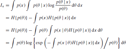
To proceed further, we suppose that is the result of our n independent observations of x and we define entropy by

(this is a function of a distribution for θ and is not a function of any particular value of θ). Then using and we see that

(the last equation results from simple manipulations as exp and log are inverse functions). It follows that we can write In in the form

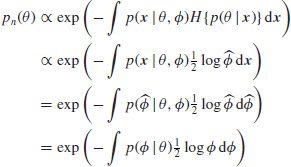
It can be shown using the calculus of variations that the information is maximized when (see Bernardo and Smith, 1994, Section 5.4.2). It follows (provided the functions involved are well behaved) that the sequence of densities

approaches the reference prior. There is a slight difficulty in that the posterior density which figures in the above expression depends on the prior, but we know that this dependence dies away as .

3.11.2 Reference priors under asymptotic normality

In cases where the approximations derived in Section 3.10 are valid, the posterior distribution is which by the additive property of Fisher’s information is . Now it is easily seen that the entropy of an density is

(writing as ) from which it follows that

to the extent to which the approximation established in the last section is correct. Thus, we have

since the approximation in the previous section shows that is negligible except where is close to θ. It follows on dropping a constant that

and so we have another justification for Jeffreys’ prior which we first introduced in Section 3.3.

If this were all that this method could achieve, it would not be worth the aforementioned discussion. Its importance lies in that it can be used for a wider class of problems and that further it gives sensible answers when we have nuisance parameters.

3.11.3 Uniform distribution of unit length

To see the first point, consider the case of a uniform distribution over an interval of unit length with unknown centre, so that we have observations , and as usual let be the result of our n independent observations of x. Much as in Section 3.5, we find that if m=min xi and M=max xi then the posterior is

For a large sample, the interval in which this is nonzero will be small and (assuming suitable regularity) will not vary much in it, so that asymptotically . It follows that

which is asymptotically equal to

Since is the maximum of n observations uniformly distributed on [0, 1] we have

from which it follows that the density of is proportional to un–1, so that and hence . Similarly we find that , so that

Because this does not depend on θ it follows that does not depend on θ and so is uniform. Taking limits, the reference prior is also uniform.

Note that in this case the posterior is very far from normality, so that the theory cannot be applied as in Subsection 3.11.2, headed ‘Reference priors under asymptotic normality’, but nevertheless a satisfactory reference prior can be devised.

3.11.4 Normal mean and variance

When we have two parameters, as in the case of the mean and variance of an distribution, we often want to make inferences about the mean θ, so that is a nuisance parameter. In such a case, we have to choose a conditional prior for the nuisance parameter which describes personal opinions, previous observations, or else is ‘diffuse’ in the sense of the priors we have been talking about.

When we want to describe diffuse opinions about given θ, we would expect, for the aforementioned reasons, to maximize the missing information about given θ. This results in the sequence

Now we found in Section 3.10 that in the case where we have a sample of size n from a normal distribution, the asymptotic posterior distribution of is N(S/n,  2S2/n3), which we may write as , and consequently (using the form derived at the start of the subsection on ‘Reference priors under asymptotic normality’) its entropy is

It follows that

In the limit we get that

In this case, the posterior for the mean is well approximated by , where and , so that the entropy is

We thus get

using the facts that is negligible except where is close to and that, of course, must equal . We note that if does not depend on θ, and so, in particular, in the case where , the density is a constant and in the limit the reference prior is also constant, so giving the usual reference prior . It then follows that the joint reference prior is

This, as we noted at the end of Section 3.3 is not the same as the prior given by the two-parameter version of Jeffreys’ rule. If we want to make inferences about with θ being the nuisance parameter, we obtain the same reference prior.

There is a temptation to think that whatever parameters we adopt we will get the same reference prior, but this is not the case. If we define the standard deviation as and the coefficient of variation or standardized mean as , then we find

(see Bernardo and Smith, 1994, Examples 5.17 and 5.26) which corresponds to

3.11.5 Technical complications

There are actually some considerable technical complications about the process of obtaining reference posteriors and priors in the presence of nuisance parameters, since some of the integrals may be infinite. It is usually possible to deal with this difficulty by restricting the parameter of interest to a finite range and then increasing this range sequentially, so that in the limit all possible values are included. For details, see Bernardo and Smith (1994, Section 5.4.4).