Chapter 7: Visualizing and Reporting Petabytes of Data

In this chapter, we will cover how to visualize data and create reports using Power BI. You will be learning how to develop reports within a Synapse workspace and link Power BI to an existing dataset.

You will also learn something very interesting – how to integrate existing Power BI reports into the Synapse workspace and visualize the data in the same place without any difficulty.

Apart from this, you will also learn performance best practices for developing your Power BI reports with a very large dataset.

We will be covering the following recipes:

• Combining Power BI and a serverless SQL pool
• Working on a composite model
• Using materialized views to improve performance

Combining Power BI and aserverless SQL pool

Azure Synapse Studio gives you the flexibility to connect to the Power BI workspace and provides you with seamless integration between data sources and reports. You can work within the Synapse workspace to create Power BI reports independently in the Power BI service.

You have the flexibility to combine multiple data sources to create a single Power BI dataset. This helps you to analyze disparate data sources and create insight by referring to a single data model. We refer to this as a Power BI linked service.

Getting ready

We will be using the same Synapse workspace that we have used throughout the book for this recipe.

The prerequisites for this recipe are as follows:

• Make sure you have Power BI Desktop downloaded and installed. You can download it from this link: https://www.microsoft.com/en-in/download/details.aspx?id=58494.
• You need to have a Power BI Pro license to develop reports and get all the benefits of Power BI features.
• We will be using the BoxOfficeMojo dataset.

How to do it…

Let's begin this recipe and see how we can bring the Power BI service into the Synapse workspace and leverage it for creating reports.

You need to link the Power BI service to the existing Synapse workspace:

1. Go to the Home tab on the Synapse Studio portal and click the Visualize tab to create a Power BI linked service, as shown in Figure 7.1:

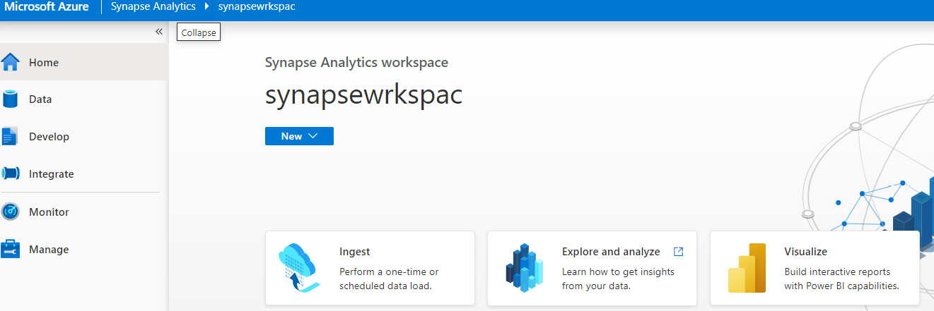
Figure 7.1 – Create a Power BI linked service

2. You can now get the option blade to provide the details that are required to create the Power BI linked service for the Synapse workspace. Please fill in all the details, as shown in Figure 7.2. You need to sign in to the Power BI account to get the Power BI Tenant and Workspace name details:

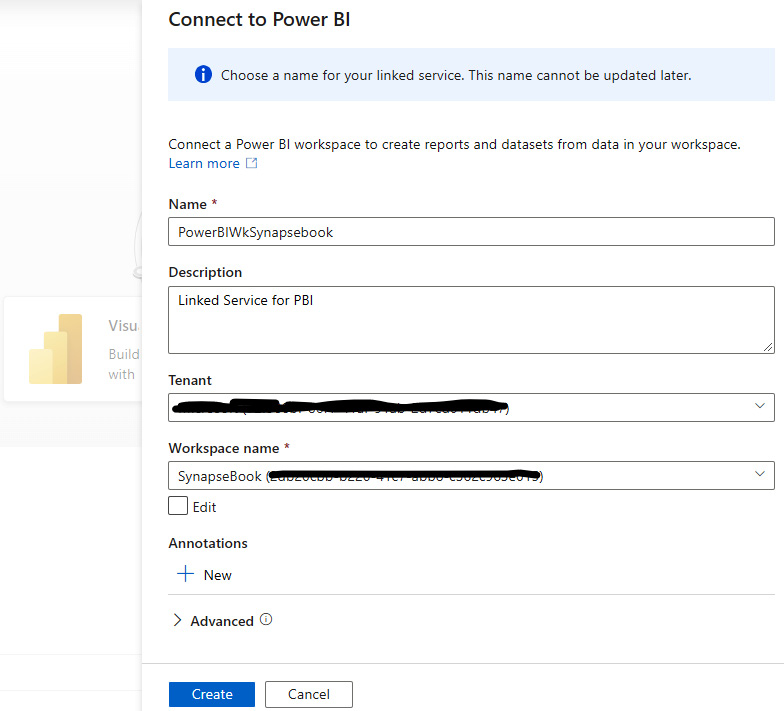
Figure 7.2 – Choose the name of your linked service

3. Go to the Manage tab in Synapse Studio and publish the Power BI linked service name PowerBIWkSynapsebook under Linked services, as shown in Figure 7.3:

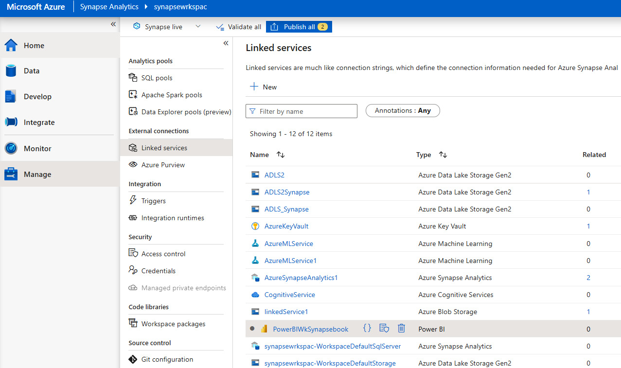
Figure 7.3 – Manage the linked service

4. Finally, you need to click on the Publish all button at the top to publish the Power BI linked service, as shown in Figure 7.4:

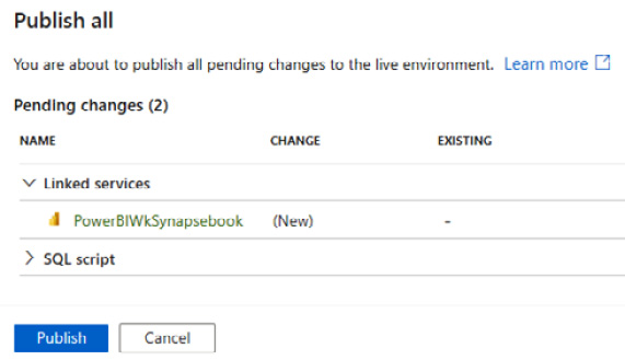
Figure 7.4 – Publishing the linked service

Now, how does it work?

How it works…

The Power BI linked service will link to the Synapse workspace, which gives you the ability to work directly and access the existing Power BI reports within Synapse Studio.

Go to the Develop tab, where you will be able to see the Power BI folder, which contains the PowerBIWkSynapsebook Power BI workspace that we have created in this recipe, as shown in Figure 7.5:

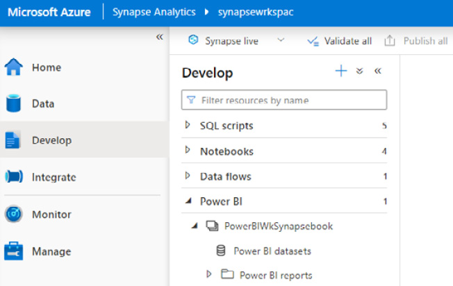
Figure 7.5 – Navigating to Power BI Workspace

You can see Power BI datasets and Power BI reports, and you can access the existing Power BI reports from the Synapse workspace directly.

In Figure 7.6, you can see that we have already an existing report name, BoxofficeMojo, in the Power BI workspace. You can access it in Synapse Studio. You can even edit the existing report and directly save it from Synapse Studio:

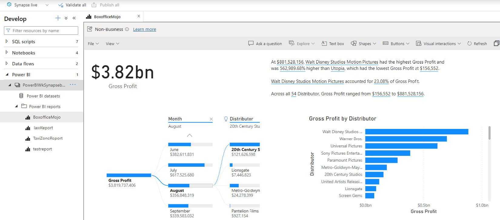
Figure 7.6 – Accessing the existing Power BI report

You can now even create a Power BI report using the SQL pool dataset and visualize it; you need to build the Power BI dataset and connect it to the Synapse pool.

Follow the following steps:

1. Click on Power BI datasets and then New Power BI dataset, as shown in Figure 7.7:

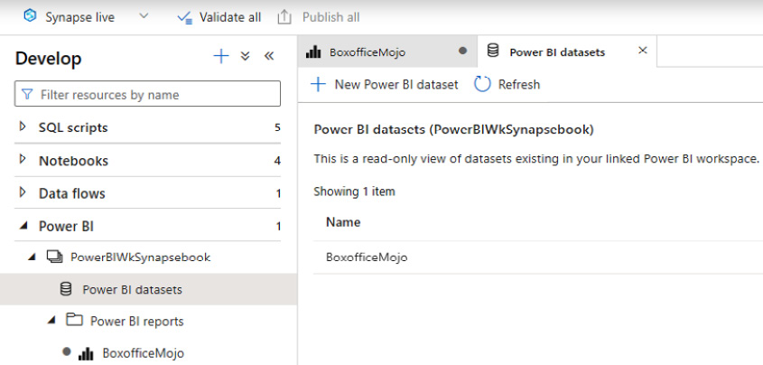
Figure 7.7 – Create a Power BI dataset

2. You need to select the data source. In our case, this will be synapsesqlpool. Click Continue:

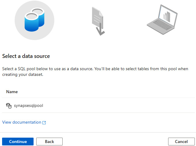
Figure 7.8 – Select the data source for creating the dataset

This will give you the option to download the .pbids (the Power BI data source) Power BI desktop file, as shown in Figure 7.9:

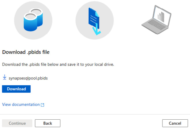
Figure 7.9 – Download the .pbids file

3. After you download the .pbids file, this will provide the connection information you need to authenticate the data source, as shown in Figure 7.10:

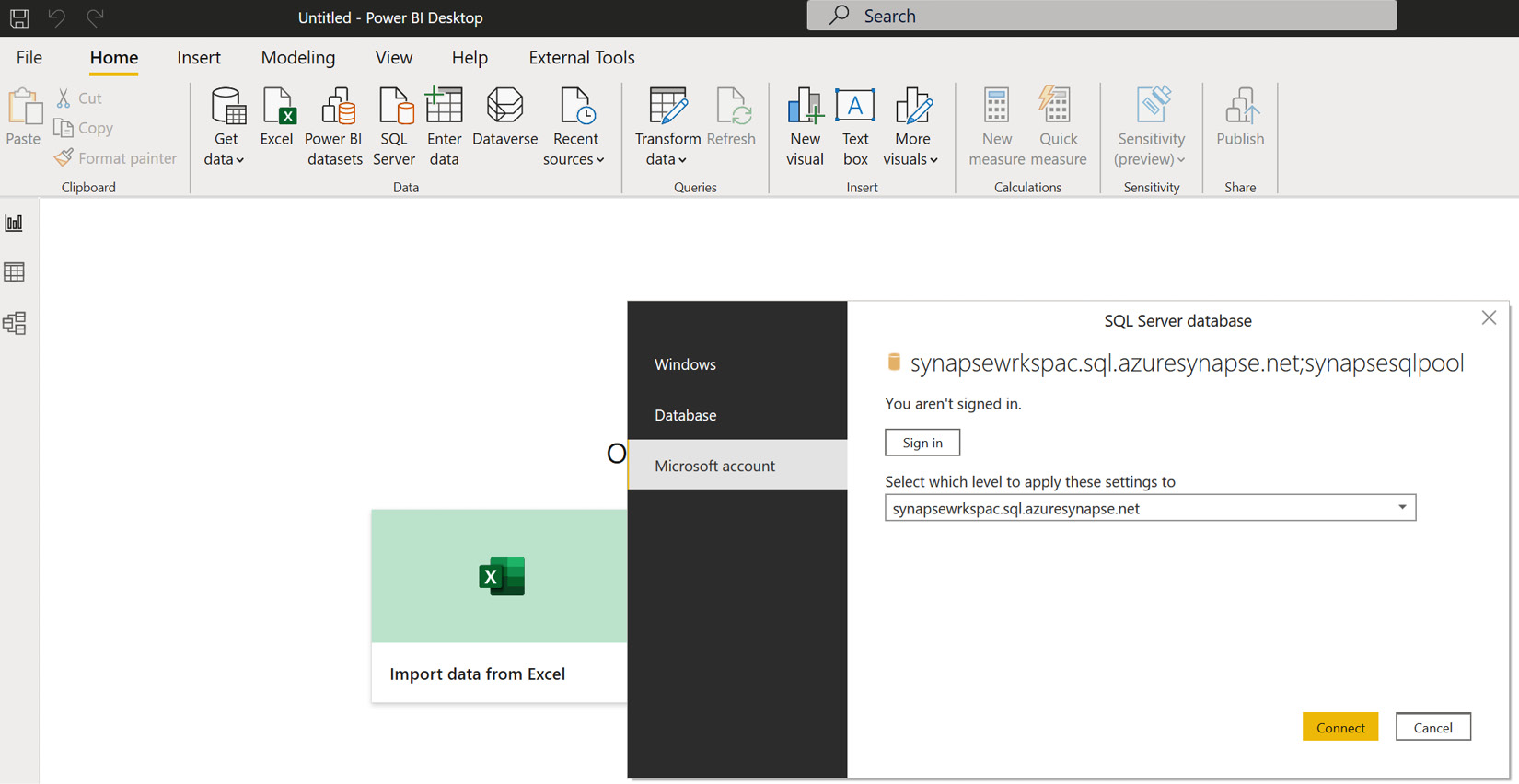
Figure 7.10 – Authenticate the data source connection

4. Once you have signed in, you can create Power BI reports using Power BI Desktop and deploy them to the same workspace, Synapsebook, in the Power BI service, as shown in Figure 7.11:

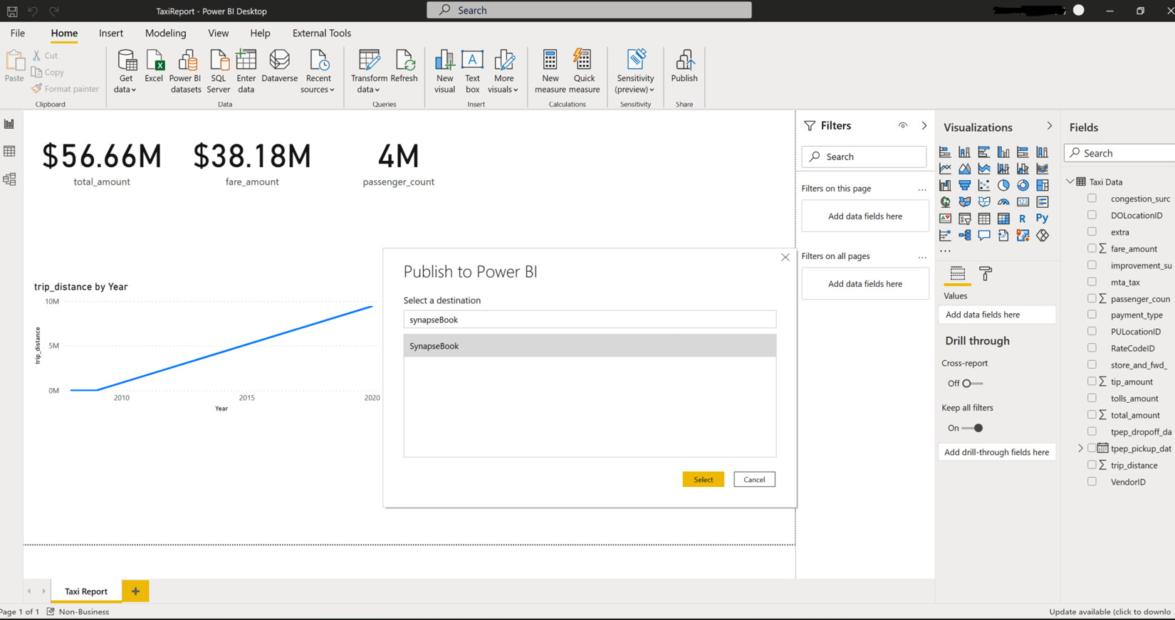
Figure 7.11 – Publish a report using Power BI Desktop

5. Finally, you should be able to access the same report from Synapse Studio, which is integrated as shown in Figure 7.12:

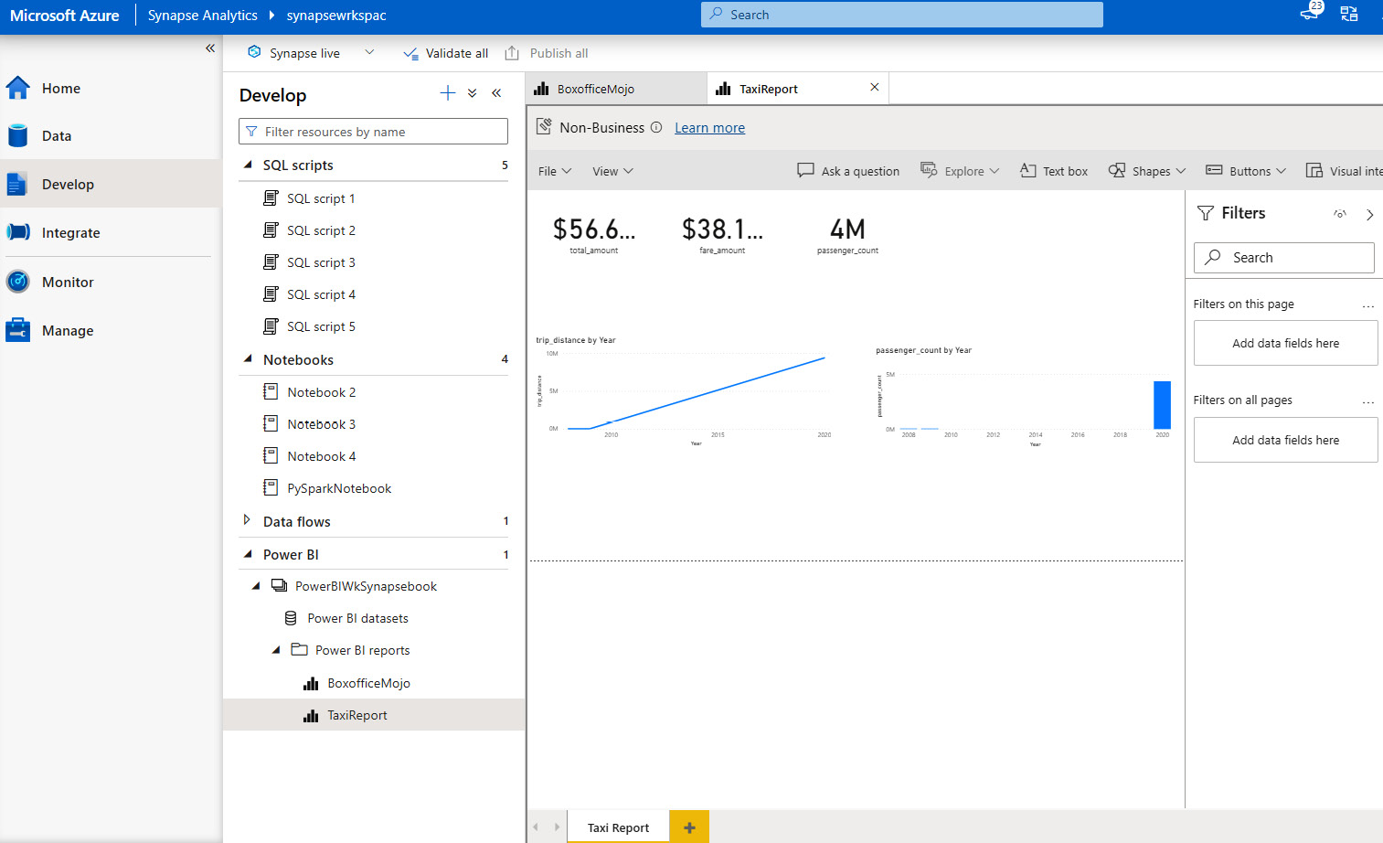
Figure 7.12 – Access the report from Synapse Studio

Working on a composite model

Let's now learn about the new Power BI composite model. With this feature, you can now add data in two different storage modes – either to a direct query or to an import. Previously, using direct query in Power BI did not allow you to add another data source to the model.

In the enterprise scenario, the data comes from multiple sources, and you will be dealing with very large datasets. With the help of composite models, you can combine large datasets and use the direct query method, as well as import data from small data sources. The advantage of this approach is that you can now handle the challenges of dealing with very large data models as well as any performance glitches.

For scenarios when you have very large data in Synapse and you also want to combine data from your local data source, you can connect Synapse data as a direct query and a local data source in import mode and join the datasets. The composite model even gives you the flexibility to do this at an entity level, which provides the most agility.

This is exactly what we will be doing in this recipe, and you will learn how to perform this using a composite model.

Getting ready

• Make sure you have Power BI Desktop installed.
• Make sure you have access to the Azure Synapse SQL pool to access data.
• Make sure you have the Power BI gateway installed.

How to do it…

Let's open a new Power BI Desktop and create a new report. We will be using both the DirectQuery method and Import mode for this recipe to build a composite model in Power BI.

Let's begin!

1. Open a new Power BI Desktop, connect to synapsesqlpool, and use DirectQuery as the connectivity mode to create the data model, as shown in Figure 7.13:

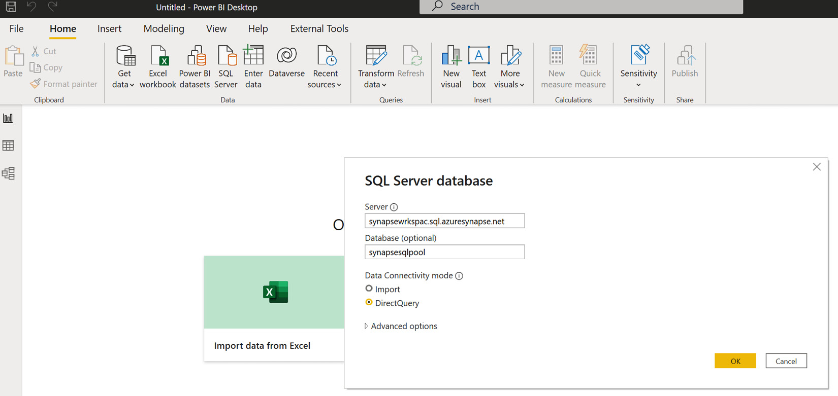
Figure 7.13 – The DirectQuery connectivity mode

2. Let's select one of the fact tables in DirectQuery mode so that we are not importing all of the data here:

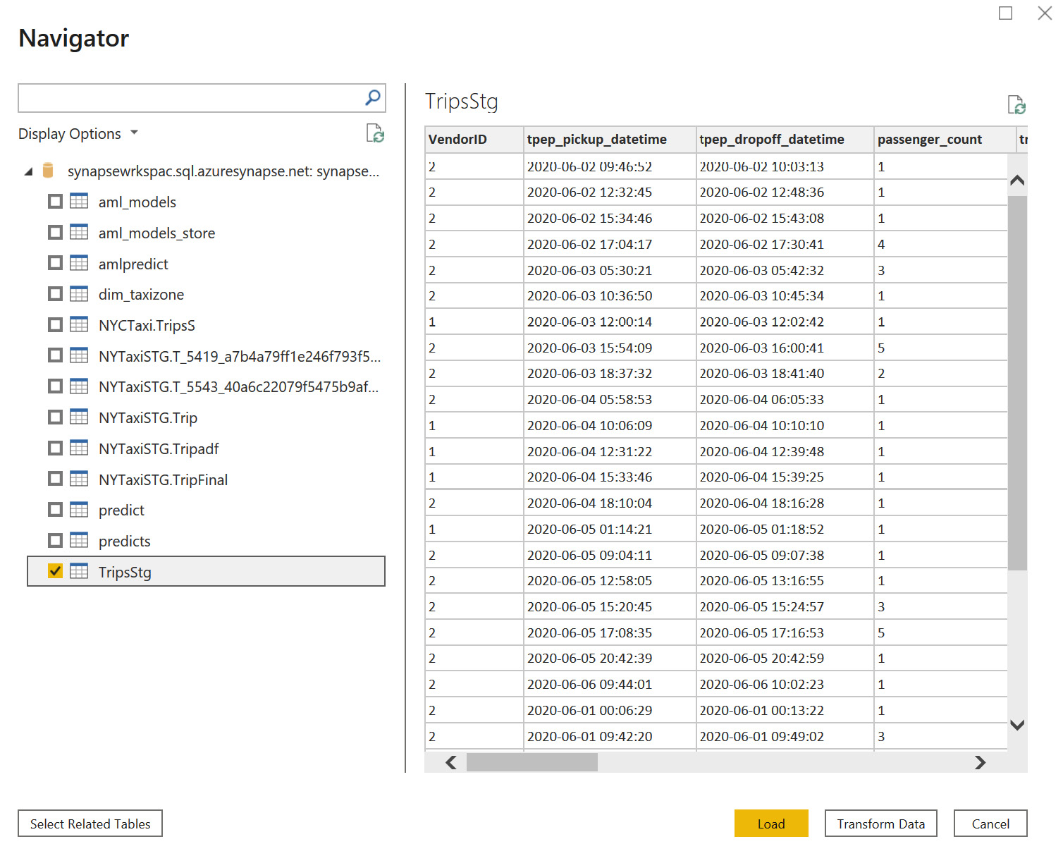
Figure 7.14 – Select the fact table to load as DirectQuery

3. Now, we will use the same synapsesqlpool database and connect the data in Import query mode, as shown in Figure 7.15:
   

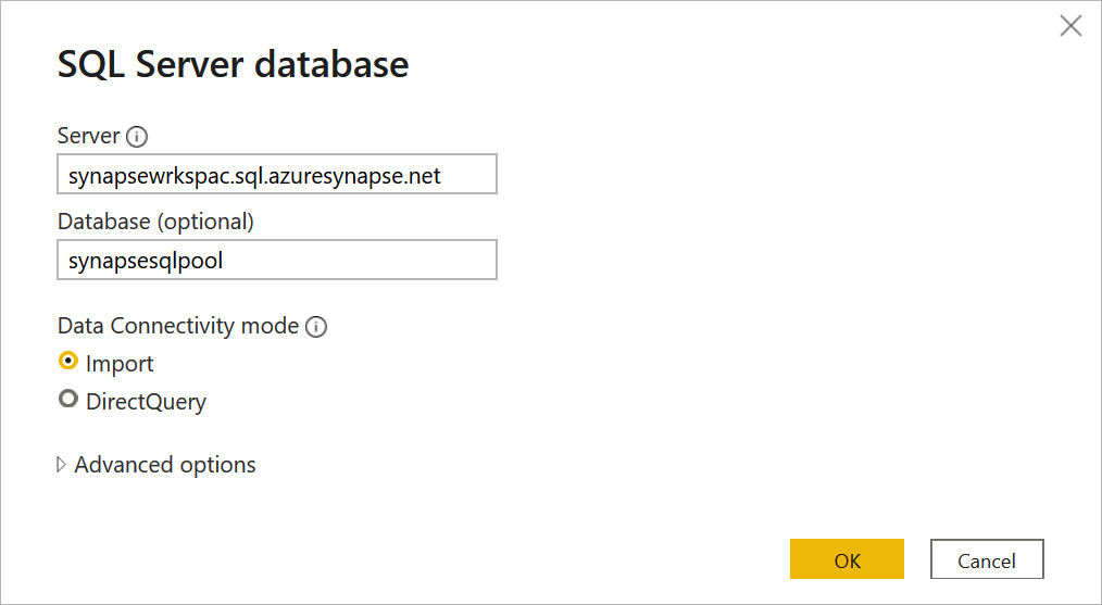
Figure 7.15 – The Import query connectivity mode

4. Now, we are going to import one of the dimension tables, since they don't contain too many records, and make the Power BI composite:

Figure 7.16 – Select a dimension table in Import query mode

5. You can now set the relationship between the two tables using LocationId, as shown in Figure 7.17:

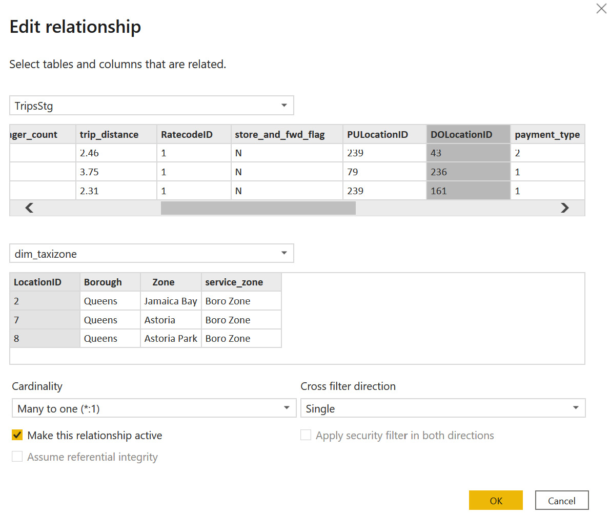
Figure 7.17 – Creating a Many to one relationship

6. This is what the final model will look like after creating a relationship between the two tables that have a composite model of data storage:

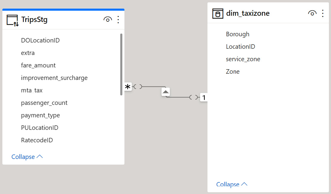
Figure 7.18 – A data model after creating a relationship

How it works…

This is one of the most interesting features of Power BI when you are dealing with a very large dataset. When you try to visualize data in the Power BI model in the form of a report, as an end user, there won't be any difference in consuming the reports, as you now have the two different storage modes within the same data model, which are Import and DirectQuery.

You can see in Figure 7.19 how Storage Mode is changed to Mixed; we can now filter the data based on the dim_taxizone dimension and filter records in the reports:

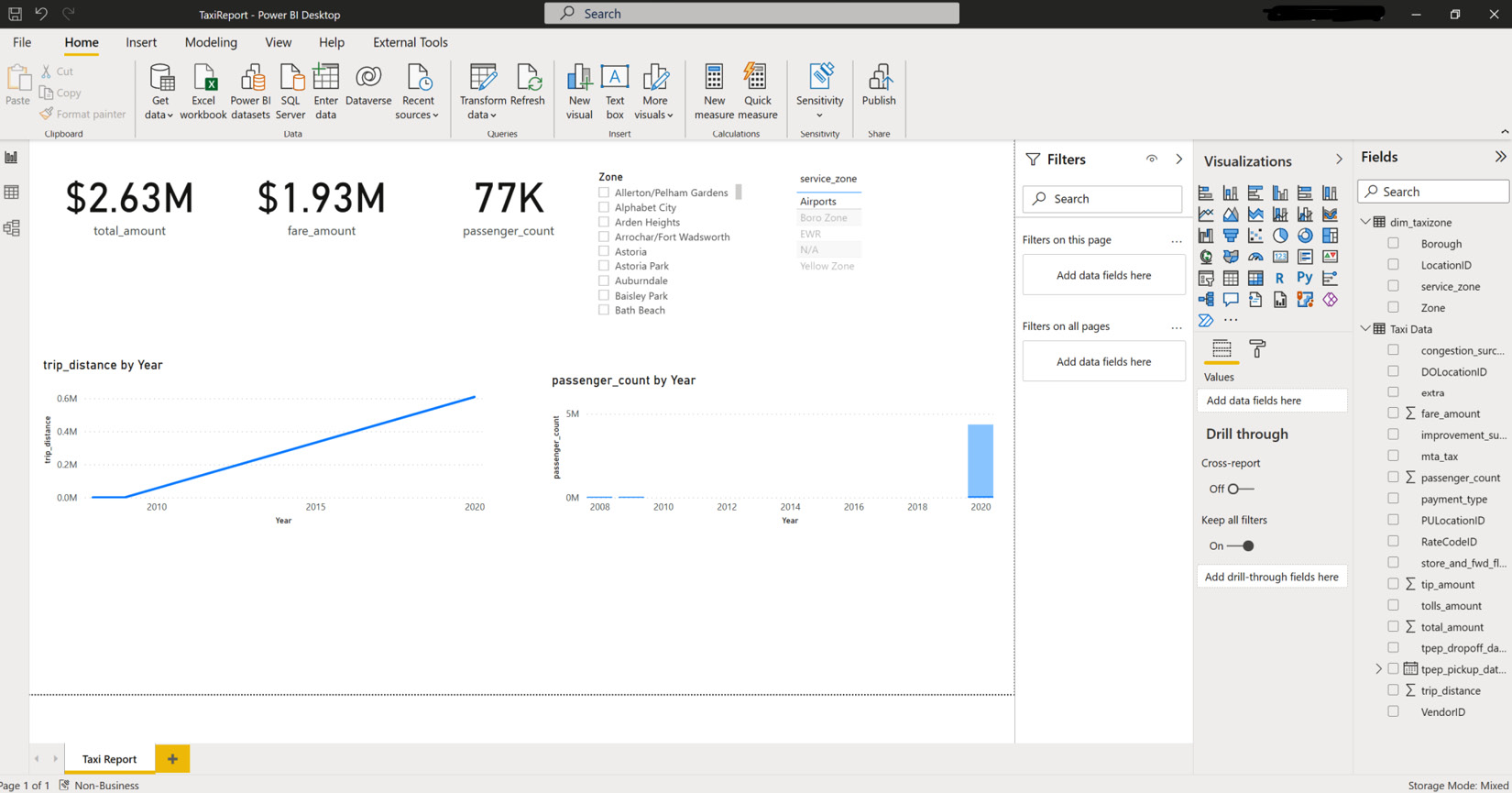
Figure 7.19 – Report creation in Mixed mode

After you deploy this report to the Synapsebook Power BI workspace name, you can access the report either from the Power BI service or the Synapse workspace, as shown in Figure 7.20:

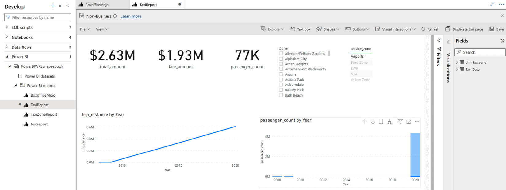
Figure 7.20 – Accessing the report from the Synapse workspace

The takeaway from this recipe is that you can combine both the DirectQuery and Import storage modes of Power BI and build a single data model. This provides the best flexibility and performance for your Power BI reports.

Using materialized views to improve performance

In this recipe, you will learn how materialized views can help in solving complex queries that are required for analytical purposes and how you can gain performance. You will learn how to create the materialized view, and when and why to use it in the SQL dedicated pool.

Materialized views are the best option in a large data warehouse, as the data is stored in a pre-processed format, unlike standard views. When you execute a query with a materialized view, it internally keeps processed data within the dedicated SQL pool, just like a physical SQL table.

Getting ready

Before you begin, make sure you have the following:

• Make sure you have the dedicated SQL pool available in the Synapse workspace.
• You need to ensure that the table in which you are creating a materialized view has a qualifying column that can participate in the columnstore index. You can refer to this document for a list of datatypes that can participate in column store index creation: https://docs.microsoft.com/en-us/sql/t-sql/statements/create-columnstore-index-transact-sql?view=sql-server-2017#LimitRest.
• Ensure you have the right permissions to create the views in the SQL pool.

How to do it…

Let's get back to the same Synapse workspace, and under the Data tab, expand the SQL pool database and let the work start on a new SQL query:

1. We will find the total gross amount by joining two tables, dim_taxizone and TripsStg, within the SQL pool, as shown in Figure 7.21.

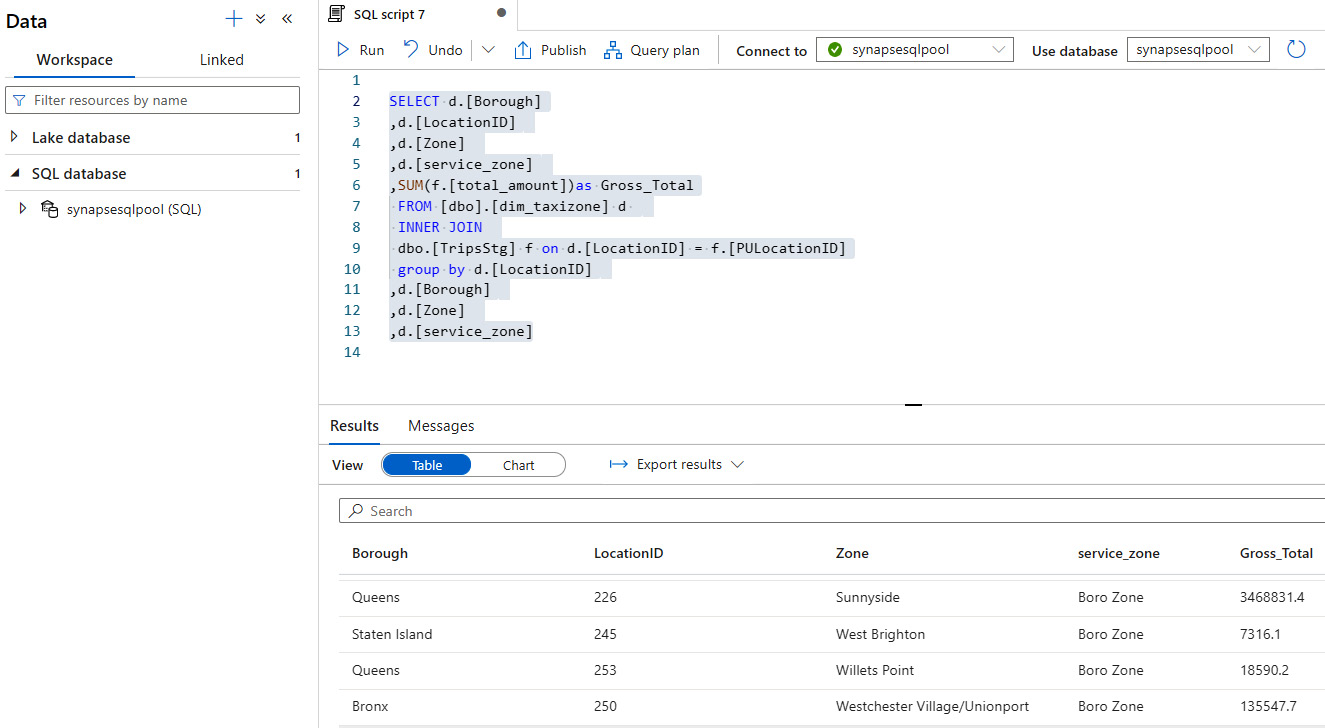
Figure 7.21 – A script to get a gross sum after joining the two tables

The SQL script can be written as follows:

SELECT d.[Borough]

,d.[LocationID]

,d.[Zone]

,d.[service_zone]

,SUM(f.[total_amount])as Gross_Total

 FROM [dbo].[dim_taxizone] d 

 INNER JOIN

 dbo.[TripsStg] f on d.[LocationID] = f.[PULocationID]

 group by d.[LocationID]

,d.[Borough]

,d.[Zone]

,d.[service_zone]

2. You now need to convert the SQL query and create a materialized view to boost the performance and get the data in a pre-compute store within the dedicated SQL pool. Refer to the following script and Figure 7.22:

   CREATE materialized view matViewGrossAmount WITH (DISTRIBUTION=HASH([LocationID])) AS

   SELECT d.[Borough]

   ,d.[LocationID]

   ,d.[Zone]

   ,d.[service_zone]

   ,SUM(f.[total_amount])as Gross_Total

    FROM [dbo].[dim_taxizone] d 

    INNER JOIN

    dbo.[TripsStg] f on d.[LocationID] = f.[PULocationID]

    group by d.[LocationID]

   ,d.[Borough]

   ,d.[Zone]

   ,d.[service_zone]

This is shown in the following screenshot:

Figure 7.22 – Create a materialized view

3. You can now verify whether the view has been created successfully, as shown in Figure 7.23:

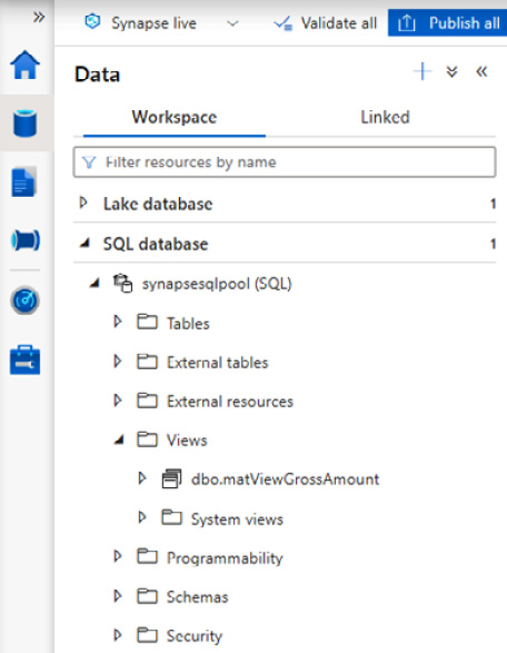
Figure 7.23 – The created materialized view

How it works…

Let's understand what we have done so far and how this works. The materialized view will act as the physical table and reduce the execution time for complex queries where we have JOINS and are using aggregated functions.

The execution plan for the query will get optimized in the dedicated SQL pool and automatically use the best-optimized execution plan.

You can get the best out of the materialized view, as the data in the view is scalable and always available compared to a regular query, where you need to depend on the individual query execution plan.

You can create the Power BI report connecting to the materialized view and get rid of the complex query in the report, which will eventually improve the overall performance of the report.

If you refer to Figure 7.24, you can see the matViewGrossAmount materialized view as the physical object, which can be loaded to Power BI for further analysis:

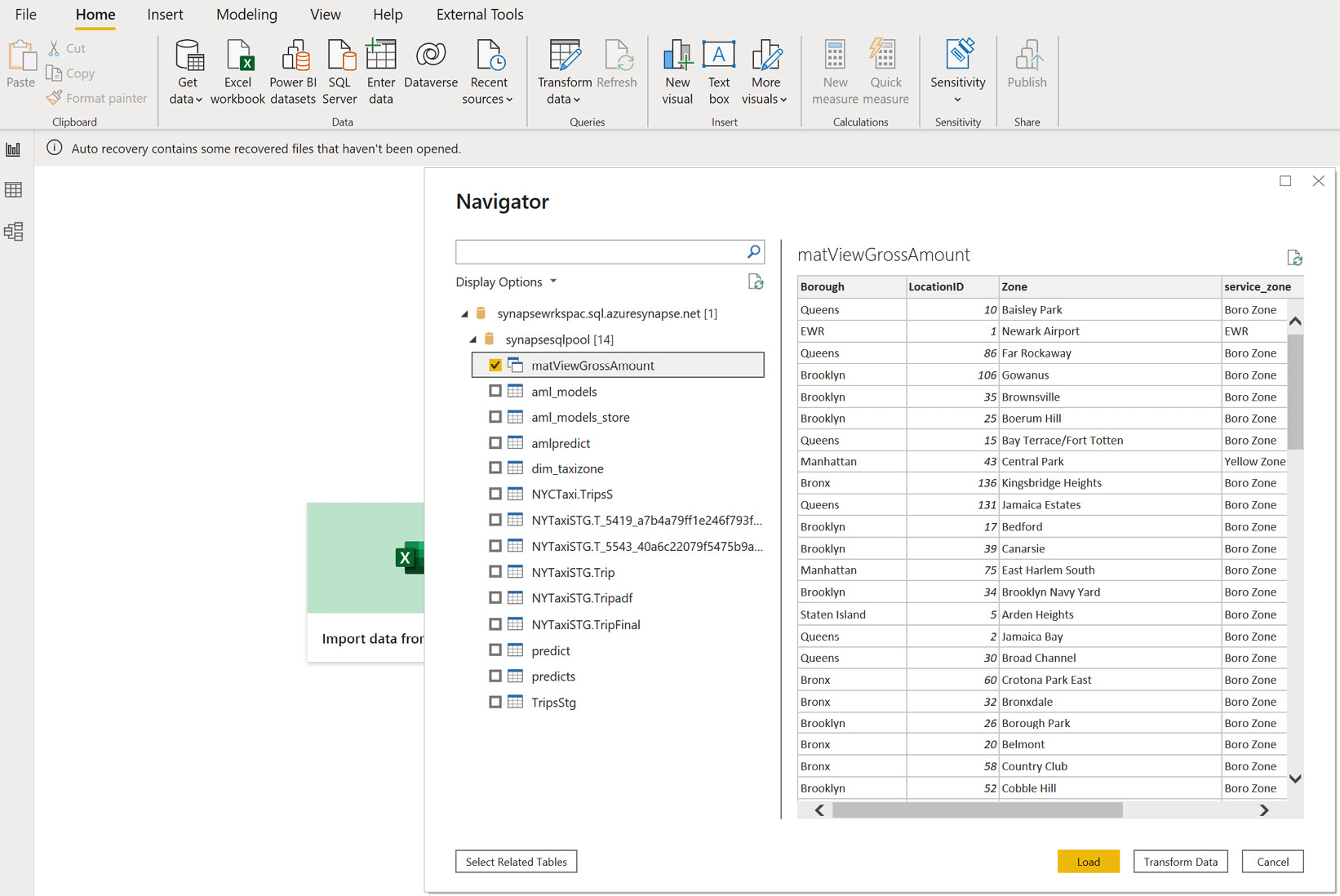
Figure 7.24 – Connected to the view in Power BI

You can create the visuals as required and get an insight within Power BI Desktop, as shown in Figure 7.25:

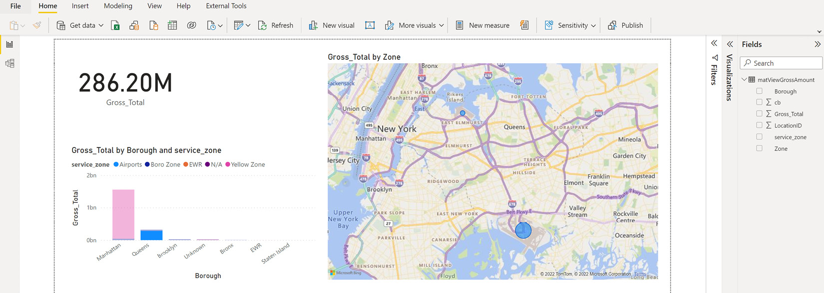
Figure 7.25 – Create a Power BI report

Finally, you can see this report in the Power BI workspace named Synapsebook; you can access the report either from the Power BI service or the Synapse workspace, as shown in Figure 7.26:

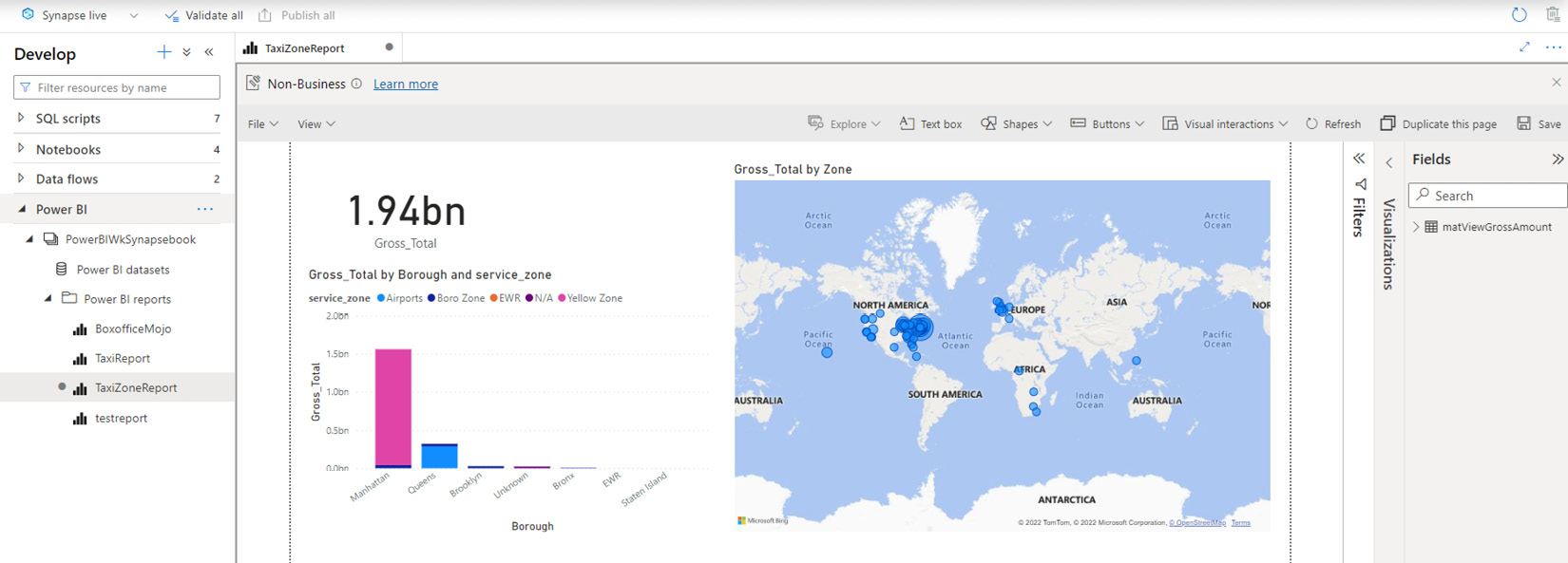
Figure 7.26 – Access the Power BI report from the Synapse workspace

The takeaway from this recipe is that the Synapse is a strong proposition for data storage, data processing, and data transformations. Power BI infuses data visualizations to Synapse for better insights and reporting.