CHAPTER 2

Artificial Intelligence/Machine Learning Project Architecture and Design

• Introduction to artificial intelligence (AI) and machine learning (ML) project architecture and design
• Illustrated steps to start an AI and ML project architecture and design perspective
• How to build and design specifically for ML and AI use cases

Chapter Outline

• Architecture and design perspective of AI and ML projects
• Comparison of current architecture and future architecture
• Data analytics and life cycle
• Data processing steps
• Future cleaning and extraction
• ML algorithms

Key Learning Points

• Learn and understand how AI and ML project architecture and design is carried over

AI and ML Project Architecture and Design Steps

• Define the problem statement
• Understand existing and current business architectures and business processes
• Define business cases and use cases
• Determine goal
• AI and ML apply to business architectures and business processes
  • Generalize the problem, use case, and business process
  • Redefine the overall process
  • Translate into AI and ML problem statements
• Define AI and ML architecture
• Evaluate the available AI and ML algorithms to decide the architecture
• Design the overall AI and ML solutions
• Design data architecture and data design
• Develop, train, validate, improve, and deploy

See Figure 2.1 AI and ML project architecture and design process for the detail architecture and design steps.

Figure 2.1 AI and ML project architecture and design process

Terms and Terminologies

An actor in the Unified Modeling Language is a role played by a user (stakeholder) or any other system that interacts with the subject. The actor interacts with the subject, for example, an organization data and the resources manipulating the data. Another example is the primary actor of a use case is the stakeholder that calls on the system to deliver one of its services.

Define Problem Statement

A problem statement is a description of an issue to be addressed or a condition to be improved upon based on the requirement in question (Jain et al. 2018). Usually, there is a gap between the current problem statement and desired goal statement of a process or product.

Look at the five W’s (who, what, when, where, and why) to define the problem statement clearly with past, present, and future states.

• Who: define the actors to the problem or system and the process involved.
• What: define the problems and the objectives of the problem.
• When: define time during the occurrence of specific event or action.
• Where: define where it happened or where it is expected to happen.
• Why: define why this is happening, why it happened, or why it will happen.

Add “how” into this mix to understand the problem clearly. Look at the big picture and analyze previous issues, current issues, and future issues. Define the desired state of how problems will be solved.

Examples of Problem Statements

ML and AI for Risk

Risks are involved in every action. It is a continuous problem to manually monitor the risks and mitigate large tasks (Rona-Tas et al., 2019). Solve this problem using ML and AI approaches.

ML and AI for Security

Security is a big problem for corporate and government organizations (McGraw et al., 2019). This problem can be solved using ML and AI approaches.

Problem statements are defined very generically and may not focus on the correct problem statements. These statements can be divided into multiple problem statements; this process is illustrated in the AI solutions for risk and AI solutions for security chapters.

Understand Existing and Current Business Architectures and Business Processes

Ask the following questions when examining old and new business architectures:

• Who are the stakeholders, customers, users, and organizations?
• How should you define your vision, strategies, tactics, policies, rules, and regulations?
• What is the value stream through initiatives and projects and how is it measured?
• What capabilities are enabled and what proposals are made using gathered information?

See Figure 2.2.

Figure 2.2 Business architecture process

Business Architecture

Business Process

Business architecture is further broken down into the business process (Vaez-Alaei et al. 2018). The business process defines how the business operates, manages, and serves to meet the businesses’ objectives. Each organization may have unique business processes in the industry and functional areas. See Figure 2.3.

Figure 2.3 Typical business process

Typically, chief executive officers are responsible for strategies, infrastructures, products, and services. Chief marketing officers are responsible for the marketing and sales domain. Chief operating officers are responsible for business operations. Nowadays, most organizations have introduced a new top management position called a chief data officer who manages data architecture, data design, data collection, data management, data processing, applying data science, ML, and AI. This role helps industries keep up with the latest technology transformations, such as moving to the Cloud infrastructure, ML, AI, and Internet of Things. In fact, all existing business processes are in the process of re-engineering and redefining to adopt technological transformations, including risk and security. All business functional areas and related business processes are at risk. This book illustrates how to automate business functional areas and related business processes using ML and AI.

Look at the retail industry business process at a very high level. See Figure 2.4.

Figure 2.4 Retail industry typical business processes

Define Business Cases

The business case must be defined for the problem statement (Haas et al. 2019). This process is illustrated for ML and AI using risk problem statements.

Problem Statements:

• Risk is everywhere. Risks are involved in every action. It is a continuous problem to manually monitor risks and mitigate, especially in the case of huge tasks. The goal is to solve this huge problem by using ML and AI approaches.
• Security is a very big problem for corporate and government organizations and could be solved using ML and AI approaches.

Identify Return on Investment (ROI) and Benefits:

Organizations will save money on a daily basis by implementing ML and AI systems for risk and security. The human workforce will be free from manually identifying and mitigating risks and security. Approximate estimation of ROI would be at least $10,000, but this number depends on the size of the organization and the current time spent on the manual risk and security tasks. ML and AI also eliminate 24/7 watchdog risk and security tasks.

Strategic Alignment:

Strategic alignment should align with business goals. The business goal of all organizations is to use the data to drive decisions and automation. The ML and AI implementation for risk and security aligns with the business goals.

Investment: The investment would be minimal as it will be Software as a Service in the Cloud.

Values:

The organization will have peace of mind. The customers and partnering organizations will have more confidence.

Efficiency:

The organization’s operational processes and automation will be improved by 60 times.

Define Use Cases

In this step, define or identify the use cases to be supported to a tangible outcome (Refactoring to Improve the Security Quality of Use Case Models 2019). Most of the ML and AI projects are diverted into research and development (R&D) projects, the reason being that use cases are identified up front. Use cases vary by industry and by business function, but some of them are listed below.

Financial and banking industry:

• Prevention of credit loss and fraud.
• Avoidance of money laundering.
• Compliance with industry standards and government clauses.

Retail industry:

• Avoidance of data breaches.
• Improve market share by competitive pricing.

Determine the Goal

The goal of ML and AI risk solutions is to capture all the risks items to identify, classify, and prioritize risks and gain prevention recommendations.

The goal of the ML and AI security solutions is to prevent threats in real time. ML and AI security systems discover, detect, provide threat scores, threat protection, and prevention recommendations.

Before going through each of the ML and AI project architecture and design steps, let us look at the typical data analytics project and its life cycle. Multiple streams of data analytics and life cycle projects may be needed to define the overall project architecture and design.

Data Analytics and Life Cycle

The data analytics life cycle is designed for large data problems and data science projects (Sahoo and Mohanty 2018). There are six phases, and the project work can occur in several phases simultaneously. The cycle is iterative to portray a real project. The work can return to previous phases as new information is uncovered. The data analytics life cycle consists of the following sequence of steps:

Data analytics life cycle overview:

1. Phase 1: Discovery
2. Phase 2: Data preparation
3. Phase 3: Model planning
4. Phase 4: Model building
5. Phase 5: Communicate results
6. Phase 6: Operationalize

The data scientist is the main analytics stakeholder. The data scientist provides analytic techniques and modeling. The other members are the team are as follows:

1. Business user: understands the domain area.
2. Project sponsor: provides high-level requirements and budgeting.
3. Project manager/agile/scrum master: ensures that objectives are met.
4. Data architect: provides business domain expertise based on deep understanding of the data.
5. Data engineer: provides technical skills, assists with data management and extraction, and supports analytic development areas.

Here are the steps that go into the process. See Figure 2.5.

Figure 2.5 Data analytics life cycle

Phase 1: Discovery

The discovery phase follows this sequence of steps:

1. Learning the business domain
2. Resources
3. Framing the problem
4. Identifying key stakeholders
5. Interviewing the analytics sponsor
6. Developing initial hypotheses
7. Identifying potential data sources

Phase 2: Data Preparation

The following elements are included in the data preparation phase:

1. This phase includes steps to explore, preprocess, and condition the data.
2. This phase creates a healthy environment and analytics sandbox.
3. Data preparation tends to be the most labor-intensive step in the analytics life cycle.
4. At least 50 percent of the time for the tasks is spent in the data preparation phase.
5. The data preparation phase is generally the most iterative and the phase that teams tend to underestimate.

The data preparation stage requires development workspaces.

Preparation of the workplace is beneficial for the following reasons:

• It creates an analytic workspace.
• It allows the team to explore data without interfering with live production data.
• A prepared workspace collects a variety of data (expansive approach).
• The workspace allows organizations to undertake ambitious projects beyond traditional data analysis.
• This concept is acceptable to data science teams and IT groups.

In the workspace, the extract, transform, load, and transform functions may be performed based on the team (System and Method for Providing Predictive Behavioral Analytics 2018):

The extract, transform, and load users may perform extract, transform, and load functions.

In the workspace, the extract, load, and transform process preserves raw data, which can be useful for examination.

Example: In a financial organizations’ credit card fraud detection, high-risk transactions may be carelessly filtered out or transformed before being loaded into the database.

Learning about the data is important for the following reasons:

1. It determines the data available to the team early in the project.
2. It highlights gaps and identifies data not currently available.
3. It identifies data outside the organization that might be useful.

Data Conditioning

The data should be conditioned for several reasons, such as cleaning data, normalizing datasets, and performing transformations. This task is viewed as the step prior to data analysis, and the step might be performed by the data owner, IT department, and database administrator. Data scientists should be involved. It is a known fact that data science teams prefer too much data rather than too little.

Here are questions and observations that must be addressed when analyzing the data, along with the chapters where you can find further information on these topics.

Chapter 3: What are the data sources and target fields?

Chapter 4: How clean is the data?

Chapter 5: How consistent are the contents and files? Are there missing or inconsistent values?

Chapter 6: Assess the consistency of the data types (numeric, alphanumeric)?

Chapter 7: Review the contents to ensure the data makes sense.

Chapter 8: Look for evidence of systematic error.

Survey and Visualize

Specific data visualization tools may be used to gain an overview of the data (Wang et al. 2019). This process starts with overview and on-demand zoom and filter details. This approach enables the user to find areas of interest and zoom and filter to find more detailed data.

The following questions and observations must be addressed when surveying and visualizing data.

Chapter 1: Review data to ensure calculations are consistent.

Chapter 2: Does the data distribution stay consistent?

Chapter 3: Assess the details of the data, the range of values, and the level of aggregation of the data.

Chapter 4: Does the data represent the population of interest?

Chapter 5: Check time-related variables: daily, weekly, monthly? Are these variables sufficient?

Chapter 6: Is the data standardized or normalized? Are the data scales consistent?

Chapter 7: In the case of geospatial datasets, are state and country abbreviations consistent?

Tools for data preparation are Hadoop, Alpine Miner, OpenRefine, Data Wrangler, and Google Cloud data preparation.

• Hadoop can perform parallel consume and analysis.
• Alpine Miner provides a graphical user interface for creating analytic workflows.
• OpenRefine (formerly Google Refine) is a free, open-source tool to use with messy data.
• Data Wrangler is an interactive tool for data cleansing and transformation.
• Google Cloud provides data preparation.

Phase 3: Data Modeling

In this phase, the following steps are conducted:

• Determine the structure of the data to help determine the tools and analytic techniques for the next phase (Palli et al. 2019).
• Determine the analytic techniques that will enable the team to meet business objectives and accept or reject the working hypotheses.
• Decide on a single model or a series of techniques as part of a larger analytic workflow.
• Understand how similar problems have been analyzed in the past.

Phase 4: Model Building

The following tasks are considered in model building:

1. Execute the models defined in Phase 3.
2. Develop datasets for training, testing, and production.
3. Develop models on training data and test-on-test data.
4. Questions to consider:

1. Does the model appear valid and accurate on the test data?
2. Does the model output and behavior make sense to the domain experts?
3. Do the parameter values make sense in the context of the domain?
4. Will the model sufficiently and accurately meet the goal?
5. Can the model avoid intolerable mistakes?
6. Are more data or inputs needed?
7. Will the type of model chosen support the run-time environment?
8. Will a different model be required to address the business problem?

Common model building tools are: R and PL/R—PL/R, Python, SQL, Octave, WEKA, SAS, SPSS Modeler, MATLAB, Alpine Miner, STATISTICA, and MATHEMATICA.

Phase 5: Communication Results

The following steps should be followed when communicating results:

1. Determine if the team succeeded or failed in its objectives.
2. Determine if the results are statistically significant and valid.
3. If the results are significant and valid, identify aspects of the results that present relevant findings.
4. Determine if the results are in line with the hypotheses.
5. Communicate the results and major insights derived from the analysis.

Phase 6: Operationalize

The following occurs in the operationalize phase:

1. The team communicates the benefits of the project.
2. The team sets up a pilot project to deploy the work in a controlled way.
3. Risks are managed and corrective action is taken by undertaking small scope and pilot deployment before a wide-scale rollout.
4. During the pilot project:

1. The team may execute the algorithm more efficiently in the database rather than with in-memory tools like R, especially with larger datasets.
2. To test the model in a live setting, consider running the model in a production environment for a discrete set of products or a single line of business.
3. Monitor model accuracy and retrain the model if necessary.

Let us look at the ML algorithms mind map and define the terms and terminologies used in the mind map.

ML Data Processing

Data processing is important in any analytical project, data project, or ML and AI project. Most of the time is spent in this step (Kotenko et al. 2019).

See Figure 2.6.

Figure 2.6 ML and AI data processing map

Some of the statistics-related items are discussed here. If you want to know more about the terms and terminologies, please reference a statistics book. Figure 2.6 explains the required steps needed to process data and lists statistical experiments and measuring methods.

The first step in the data processing is to determine the statistical data type or levels of measurement by examining different techniques (Overgoor et al. 2019; Ohanian 2019).

Nominal Data

Nominal data (also known as nominal scale) is a type of data used to label variables without providing any quantitative value. It is the simplest form of a scale of measure. Unlike ordinal data, nominal data cannot be ordered or measured. Qualitative classifications include variables such as city, name, state, or any categorical data, which has a numerical representation tied to a categorical attribute value. For example, the gender field in a table (0 = Unavailable, 1 = Male, and 2 = Female). These identifiers represent actual attribute values. Nominal data type should not be applied with any mathematical operations. The order is not a valid. The central tendency for nominal data type is mode.

Ordinal Data

Ordinal data are orderable or can be ranked; for example: 0 = low, 2 = high, and 1 = medium. With ordinal data, the ordering is very important and central tendency to ordinal data is mode or median.

Interval Data

The items should also be measured to quantify and compare differences between them. For example, temperature as measured in Fahrenheit or Celsius.

Interval scales are numeric scales where both the order and the exact differences are valid. For example, the difference between 60 and 50 degrees is a measurable 10 degrees, as is the difference between 80 and 70 degrees. The central tendency can be measured by mode and median, and standard deviation can also be calculated.

Ratio Data

Ratio data are any numeric data that is measurable, orderable, can be ranked, and can be applied to any mathematical calculation. For example: height, weight, duration, sales amount, and profit amount. The central tendency for the ratio data is mode, mean, median, average, and orderable. See Table 2.1.

Table 2.1 Ratio data

Provides	Nominal	Ordinal	Interval	Ratio
Order of value	No	Yes	Yes	Yes
Frequency distribution (count)	Yes	Yes	Yes	Yes
Mode	Yes	Yes	Yes	Yes
Median	No	Yes	Yes	Yes
Mean	No	No	Yes	Yes
Quantify the difference	No	No	Yes	Yes

Data Exploration

Data exploration analyzes data using visual exploration to understand the dataset and determine data characteristics such as size, amount of data, completeness of the data, correctness of the data, and the relationship between data elements (Alvarez-Ayllon 2018).

Variable Identification

Variable identification is the basis for any input (predicator) or output (target) to ML models. Variable identification determines what kind of variables can be used as a predicator or target.

Univariate Analysis

Univariate analysis is a statistical analysis that determines the variable or multiple variables involved. This analysis applies to categorical variables and features (qualitative) or numerical (quantitative) univariate data. Categorical univariate data consist of numbers such as height or weight.

Typically, univariate is visualized using a frequency distribution table, bar chart, histograms, frequency polygons, and pie charts.

1. Continuous features
2. Categorical features

Bivariate Analysis

Bivariate analysis is the statistical analysis of two variables (attributes) and explores the relationship between two variables. Bivariate analysis determines the strength of the association between variables. This analysis examines the differences between two variables and the significance of the differences.

Types of bivariate analysis include numerical versus numerical, categorical versus categorical, and numerical versus categorical. Bivariate analysis is illustrated through any one of the following visualizations.

Scatter Plot

A scatter plot explores two numerical values to provide a visual representation of the linear and nonlinear relationships.

Linear correlation quantifies the strength of a linear relationship using the following formula.

where x(dash) and y(dash) are the sample mean, and n is the number of samples.

Correlation Plot

Correlation plots are used to assess whether or not correlations are consistent across groups.

1. Two-way table
2. Stacked column chart

Chi-Square Test

Chi-square test is a statistical hypothesis test where the sampling distribution of the test statistic is a chi-squared distribution when the NULL hypothesis is true. The Pearson’s chi-square test is commonly used. The chi-square test is used to determine if a significant difference exists between the expected frequencies and the observed frequencies in one or more categories. The chi-square test gives P value.

Chi-square formula:

Z-Test/T-Test

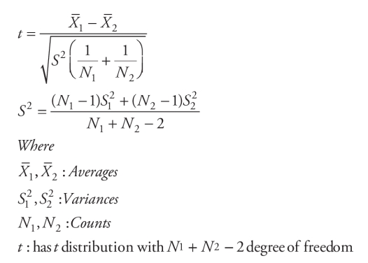
The Z-test and T-test are the same. It is a statistical evaluations of the averages of two groups and determines the differences and significance of the differences.

Analysis of Variance (ANOVA)

The ANOVA is a short form variance test that statistically measures the averages of more than two groups that are statistically different from each other. In simple terms, the test determines the statistically significant differences between the mean values of three or more independent groups.

Feature Cleaning

Feature cleaning is another name for data cleaning. Clean and quality data determine the success of a data project. Collecting quality data is the biggest challenge.

Missing values

Null values, spaces, or no value can be present in the data.

Obvious Inconsistencies

Inconsistent data problems arise when various information systems are collecting, processing, and updating data due to human or equipment reasons.

Inconsistent data make it impossible to obtain correct information from the data and reduce data availability.

Special Values

The special values are specific to the respective dataset. For example, some default values for a date field are represented as “1900-01-01” for effective begin date and “2099-12-31” for effective end date.

Outlier

In statistics, an outlier is a data point that differs significantly from other observations (Huang et al., 2019). An outlier can cause serious problems in statistical analysis and feature cleaning.

Feature Imputation:

• Hot deck
• Cold deck
• Mean substitution
• Regression

Feature Engineering:

• Decompose
• Discretization
• Continuous features
• Categorical features
• Reframe numerical quantities
• Crossing

Feature Selection:

• Correlation
• Dimensionality reduction
• Principal component analysis (PCA)
• Singular value decomposition (SVD)
• Importance
• Filter methods
• Wrapper methods
• Embedded methods

Feature Encoding:

• Label encoding
• One hot encoding

Feature Normalization:

• Rescaling
• Standardization
• Scaling to unit length

Dataset Construction:

• Training dataset
• Test dataset
• Validation dataset
• Cross-validation

ML Algorithm Mind Map

See Figure 2.7.

Figure 2.7 ML algorithm mind map

ML Algorithms

A ML algorithm is a method used to process data to extract patterns that can be applied in a new situation (Andriosopoulos et al. 2019). The goal is to apply a system to a specific input–output transformation task.

ML and deep learning are embraced by ML algorithms. ML is a class of methods for automatically creating models from data. ML algorithms turn a dataset into a model, which is effective with supervised, unsupervised, classification, and regression algorithms.

Typical examples are real-valued labels, which are the amount of rainfall or the height of a person. The first five algorithms are linear regression, logistic regression, classification and regression trees, Naïve Bayes, and k-nearest neighbors algorithm. These algorithms are examples of supervised learning.

Classification

Gmail is an e-mail application by Google that uses ML techniques to determine if an e-mail received is a spam based on the sender, recipients, subject, and message body of the e-mail. Classification takes a set of data with known labels and labels new records based on that information.

Further classification is a family of supervised ML algorithms that designate input as belonging to a predefined class.

Some common use cases for classification include:

1. Credit card fraud detection.
2. E-mail spam detection.
3. Classification data are labeled, for example: spam and nonspam or fraud and nonfraud. ML assigns new data to a class.
4. Classification based on predetermined features.
5. Features the “if” questions.
6. The label answers the “if” questions, for example: if it walks, flies, and whistles like a bird, the label is “bird.”

Clustering

Clustering can be used for search results grouping, grouping of customers, anomaly detection, and text categorization.

Google News uses a technique called clustering to group news articles into categories based on title and content. Clustering algorithms discover groupings that occur in collection of data. Clustering places objects into categories by analyzing similarities between inputs.

Clustering uses unsupervised ML algorithms that do not have the outputs in advance:

1. Clustering uses the K-means algorithm to initialize all the coordinates to centroids.
2. With every pass of the algorithm, each point is assigned to its nearest centroid based on some distance metric, usually Euclidean distance.
3. The centroids are updated to be the “centers” of all the points assigned to it in that pass.
4. This process repeats until a minimum change in the centers occurs.

K-means Clustering

The K-means clustering algorithm is popular because it can be applied to relatively large sets of data. The user specifies the number of clusters to be found and the algorithm separates the data into spherical clusters by finding a set of cluster centers, assigning each observation to a cluster, and determining new cluster centers.

The sample space is initially partitioned into K-clusters and the observations are randomly assigned to the clusters. For each sample, the distance from the observation to the centroid of the cluster should be calculated. If the sample is closest to its own cluster, leave it or select another cluster.

Repeat steps 1 and 2 until no observations are moved from one cluster to another. When the clusters are stable, each sample is assigned a cluster, which results in the lowest possible distance to the centroid of the cluster.

Collaborative Filtering

Amazon uses a ML technique called collaborative filtering (commonly referred to as recommendation) to determine which products users will like based on their history and similarity to other users who bought similar products.

Collaborative filtering algorithms recommend items based on preference information from many users. The goal of a collaborative filtering algorithm is (a) to take preferences data from users and (b) to create a model that can be used for recommendations or predictions.

Random Forests

Random forests or random decision forests are a collective learning method for classification, regression, and other tasks. These forests operate by constructing a multitude of decision trees at training time and outputting the mode of the classes (classification) or mean prediction (regression) of the individual trees. Random decision forests compensate for decision trees’ habit of overfitting their training set.

Association Rules

The association rules are the statements that show the probability of relationships between data items in large datasets in various types of databases. Association rule mining has several applications and is widely used to help discover sales correlations in transactional data or discover diagnoses in medical data. Other applications use associated rules in decision making.

Regression

Regression is used frequently in finance statistical measurements, investing, and other disciplines that attempt to determine the strength of the relationships between one dependent variable (usually denoted by Y) and a series of other changing variables (known as independent variables) (Liu et al. 2019).

Typical regressions such as linear regression can be used to quantify the relative impacts of age, gender, and diet (the predictor variables) on height (the outcome variable). Linear regression is also known as multiple regression, multivariate regression, ordinary least squares, and regression. Regression techniques are used for predictive modeling and data mining tasks. On average, only two or three types of regression are commonly used.

Linear Regression

Linear regression is a ML algorithm based on supervised learning. Regression models target prediction values based on independent variables. This algorithm is mostly used to examine the relationship between variables and forecasting. Regression models differ based on the relationship between the dependent and independent variables and the number of independent variables being used.

Linear regression predicts the value of a dependent variable (y) based on a given independent variable (x). This regression technique discovers the linear relationship between x-input and y-output.

Linear regression is used in statistical calculations. In simple linear regression, a single independent variable is used to predict the value of a dependent variable. In multiple linear regression, two or more independent variables are used to predict the value of a dependent variable. The difference between the two is the number of independent variables.

Linear regression can be used to model the relationship between two variables by fitting a linear equation to observed data. One variable is an explanatory variable, and the other is a dependent variable. For example, a modeler might want to relate the weights of individuals to their heights using a linear regression model.

Before attempting to fit a linear model to observed data, a modeler should first determine if there is a relationship between the variables of interest. This does not necessarily mean that one variable causes the other (e.g., higher exam passing scores do not cause higher college grades); however, some significant association is present between the two variables. A scatterplot may be used to determine the strength of the relationship between two variables. If there appears to be no association between the proposed explanatory and dependent variables (i.e., if the scatterplot does not indicate an increasing or decreasing trends), fitting a linear regression model to the data will not provide a useful model. This means another approach, such a problem solution, should be used.

A valuable numerical measure of association between two variables is the correlation coefficient, which is a value between −1 and 1, indicating the strength of the association of the observed data for the two variables. Let us demonstrate how it works out. A linear regression line has an equation of the form Y = a + bX, where X is the explanatory variable and Y is the dependent variable. The slope of the line is b, and a is the intercept (the value of y when x = 0).

Logistic Regression

Logistic regression is named for the function used at the core of the method: the logistic function. The logistic function is also called the sigmoid function. This function was developed by statisticians to describe properties of population growth in ecology. It is an S-shaped curve that can take any real-valued number and map it into a value between 0 and 1, but never exactly at those limits.

Ordinary Least Square Regression (OLSR)

The OLSR is a generalized linear modeling technique. It is used for estimating all unknown parameters involved in a linear regression model. This technique minimizes the sum of the squares of the difference between the observed variables and the explanatory variables. OLSR is one of the simplest methods of linear regression. The goal of OLSR is to closely fit a function with the data. It is carried out by minimizing the sum of squared errors from the data.

Stepwise Regression

Stepwise regression is a method of fitting regression models with predictive variables carried out by an automatic procedure. In each step, a variable is considered for addition or subtraction from the set of explanatory variables based on specified criterion.

Let us examine an example of how the stepwise regression procedure works by considering a dataset that concerns the hardening of the cement. The goal in this example is to learn how the composition of the cement and the heat evolved during the hardening of the cement. Data were measured and recorded for 13 batches of cement:

Response y: Heat evolved in calories during hardening of cement on a per gram basis.

Predictor x1: Percent of tricalcium aluminate.

Predictor x2: Percent of tricalcium silicate.

Predictor x3: Percent of tetracalcium alumino ferrite.

Predictor x4: Percent of dicalcium silicate.

Subsequent steps will need to be taken to arrive at the solution.

Multivariate Adaptive Regression Splines

Multivariate adaptive regression splines is a form of regression analysis introduced by Jerome H. Friedman in 1991. It is a nonparametric regression technique and is an extension of linear models that automatically model nonlinearities and interactions between variables.

Time Series Analysis

Time series analysis develops models that best capture or describe an observed time series to understand the underlying causes. This field of study seeks the “why” behind a time series dataset. It is a sequence of well-defined data points measured at consistent time intervals over a period. This method is used to analyze time series data and extract meaningful statistics and characteristics about the data. This method requires one to make assumptions about the form of the data and decompose the time series into constitution components. The quality of a descriptive model is determined by how well the model describes all available data and how the model better informs the problem domain.

Time series analysis consists of analyzing time series data to extract meaningful statistics and other characteristics of the data. It has the capability to forecast the use of a model to predict future values based on previously observed values.

Text Analysis

Text analysis is a method of communication used to describe and interpret the characteristics of a recorded or visual message. The purpose of textual analysis is to describe the content, structure, and functions of the messages embedded in texts.

Prediction

In simple terms, a prediction is a forecast. A prediction can be made with many things, such as a football match or the weather. In the word prediction, “pre” means before and diction is the act of commenting on something. This leads to a guess that may be based on evidence or facts.

Simple steps to determine a prediction are:

1. Collect data using meaningful senses and use senses to make observations.
2. Search for patterns of behavior and or characteristics.
3. Develop statements about what the future observations will be.
4. Test the prediction and observe what happens.

The best way to predict with ML is to approach the problem by hiding the uncertainty related to that prediction.

Prediction intervals provide a way to quantify and communicate the uncertainty in a prediction. Confidence intervals can be used to quantify the uncertainty in the dataset population. The mean and standard deviation can be used as parameters for each of the prediction items in question.

A prediction interval can be estimated analytically for simple models, but are more challenging for nonlinear ML models.

Anomaly Detection

Anatomy detection identifies unusual items, events, or observations that may be suspicious in a dataset; typically, the anomalies tend to be a problem. Anomalies can create security issues in an organization. Network issues have been associated with bursts of activities. The patterns do not add up to the common statistical definition of an outlier. This may create failure in unsupervised methods but can be aggregated appropriately to obtain expected results. The cluster analysis algorithm may be used to detect the microcluster pattern successfully. Anomaly techniques are broken into three categories: unsupervised anomaly detection, supervised anomaly detection, and semi-supervised anomaly detection.

Deep Learning

Deep learning is sometimes referred to as structured learning or hierarchical learning. Deep learning is part of ML methods based on artificial neural networks. The learning can be supervised, semi-supervised, or unsupervised.

Neural Network Types

There different neural networks are shown in Figure 2.8.

Figure 2.8 Neural network types

Deep Boltzmann Machine (DBM)

The DBM is also called stochastic Hopfield network with hidden units. It is the first neural network capable of learning internal representations and can represent and solve difficult combinatoric problems. It is named after the Boltzmann distribution in statistical mechanics, which is used in their sampling function.

The DBM has the following features:

• An unsupervised, probabilistic, generative model with entirely undirected connections between different layers.
• Contains visible units and multiple layers of hidden units.
• Like result-based management, no intralayer connection exists in DBM; connections only exist between units of the neighboring layers.
• A network of symmetrically connected stochastic binary units.
• DBM can be organized as a bipartite graph with odd layers on one side and even layers on the other.
• Units within the layers are independent of each other but are dependent on neighboring layers.
• Learning is made efficient with layer-by-layer pretraining.
• DBM is fine-tuned by backpropagation after learning the binary features in each layer.

Deep Belief Network

A deep belief network is a generative graphical model and is referred as a class of deep neural networks. The network is composed of multiple layers of latent variables with connections between the layers, but not between units in each layer. If trained on a set without supervision, a deep belief network can learn to probabilistically reconstruct its inputs and act as a feature detector. After this learning step, the network can be further trained with supervision to perform classification.

Convolutional Neural Network

The convolutional neural network is a type of artificial neural network used in image recognition and processing and is specifically designed to process pixel data. A neural network is a system of hardware or software patterned after the operation of neurons in the human brain. A convolutional neural network is a category of neural networks that are very effective in areas such as image recognition and classification.

These networks are used in a variety of areas, including image and pattern recognition, speech recognition, natural language processing (NLP), and video analysis.

Stacked Autoencoders

A stacked autoencoder is a neural network that consists of multiple layers of light autoencoders where the outputs of each layer are wired to the inputs of the successive layer. The stacked autoencoder can be used for classification problems.

Ensemble

An ensemble is a type of supervised learning.

ML examples include medical diagnosis, image processing, prediction, classification, learning association, and regression. The intelligent systems built on ML algorithms have the capability to learn from experience or historical data. A large amount of data is recommended because it provides better insights.

The ensemble is a method used in learning algorithms to construct a set of classifiers and to classify new data points by taking a weighted vote of their predictions. The original ensemble method is Bayesian averaging, but more recent algorithms include error-correcting output coding, bagging, and boosting. Bagging is a way to decrease the variance in the prediction by generating additional data using combinations with repetitions to produce multi-sets of the original data.

Random Forest

Random forest—sometimes referred to as a random decision forest—is a popular ensemble method and can be used to build predictive models for both classification and regression problems. Ensemble methods use multiple learning models to gain better predictive results. Random forest models create an entire forest of random, uncorrelated decision trees to arrive at the best possible answer.

Gradient Boosting Machines

Gradient boosting is one of the most powerful techniques for building predictive models.

The boosting method converts weak learners into strong learners. Each new tree is a fit on a modified version of the original dataset. AdaBoost can be introduced for training purposes, beginning with the AdaBoost Algorithm. The weights are increased for observations after evaluating the first tree. Computation is done to determine classification errors from the second tree. A third tree helps predict the revised residuals. The final ensemble model is created after a specified number of iterations.

Boosting

Boosting is a ML ensemble meta-algorithm for reducing bias and variance in supervised learning. Boosting is a family of ML algorithms that converts weak learners to strong ones.

Bootstrapped Aggregation (Bagging)

The goal of an ensemble model is to bring a group of weak learners together to form a strong learner. Bagging is used when the goal is to reduce the variance of a decision tree. This creates several subsets of data from the sample dataset.

AdaBoost

AdaBoost—also referred to as adaptive boosting—is the first practical boosting algorithm proposed by Freund and Schapire in 1996. AdaBoost focuses on classification problems and aims to convert a set of weak classifiers into a strong one.

Stacked Generalization (Blending)

Stacked generalization is simply a general method of using a high-level model to combine lower level models to achieve greater predictive accuracy. The first step is to collect the output of each model into a new set of data.

Gradient Boosted Regression Trees

Gradient boosting is a ML technique used for regression and classification problems. This technique produces a prediction model in the form of an ensemble of weak prediction models, typically decision trees.

Neural Networks

A neural network is a series of algorithms that recognizes underlying relationships in a set of data using a process that imitates the way the human brain operates. Neural networks can adapt to changing input. The network generates the best possible result without needing to redesign the output criteria.

Radial Basis Function Network

A radial basis function network is a mathematical modeling, radial basis function network that uses radial basis functions as activation functions. The network’s output is a linear combination of radial basis functions of the inputs and neuron parameters.

Perceptron

Perceptron is a ML algorithm that provides classified outcomes for computing. It dates back to the 1950s and represents a fundamental example of how ML algorithms develop data.

Backpropagation

Backpropagation requires the derivatives of activation functions to be known at network design time. Backpropagation is commonly used by the gradient descent optimization algorithm to adjust the weight of neurons by calculating the gradient of the loss function.

Hopfield Network

The Hopfield network is a recurrent artificial neural network popularized by John Hopfield in 1982 but described earlier by Little in 1974. The Hopfield nets serve as content-addressable (“associative”) memory systems with binary threshold nodes.

Regularization

Regularization is a form of regression that constrains, regularizes, or shrinks the coefficient estimates toward zero. This technique discourages learning a more complex or flexible model to avoid the risk of overfitting. Regularization illustrates that models that overfit the data are complex models that often have too many parameters.

Ridge Regression

Ridge regression is a technique for analyzing multiple regression data that suffer from multicollinearity. When multicollinearity occurs, least squares estimates are unbiased but their variances are large. Multicollinearity (also known as collinearity) is a one-predictor variable in a multiple regression model that can be linearly predicted from others with a substantial degree of accuracy. Multicollinearity generally occurs when there are high correlations between two or more predictor variables. Examples of correlated predictor variables are a person’s height and weight, age and sales price of a car, years of education, and annual income.

Least Absolute Shrinkage and Selection Operator (LASSO)

LASSO is a regression analysis method that performs variable selection and regularization to enhance the prediction accuracy and interpretability of the statistical model it produces. The LASSO method was originally introduced in geophysics literature in 1986, and later independently rediscovered and popularized in 1996 by Robert Tibshirani, who used the term and provided further insights into the observed performance. The LASSO method was originally formulated for least squares models and later revealed a substantial amount about the behavior of the estimator and its relationship to ridge regression.

Elastic Net

The elastic net is a regularized regression method that linearly combines the L1 and L2 penalties of the LASSO and ridge methods. Elastic net regularization method includes both LASSO (L1) and Ridge (L2) regularization methods. Overfitting is the core idea behind ML algorithms; the goal is to build models that can find generalized trends within the data. Regularization is used to prevent overfitting the model to training data.

Least Angle Regression

Least angle regression is an algorithm for fitting linear regression models to high-dimensional data. This method was developed by Bradley Efron, Trevor Hastie, Iain Johnstone, and Robert Tibshirani. This statistical algorithm uses a linear combination of a subset of potential covariates to determine a response variable. The least angle regression algorithm produces an estimate of which variables to include, as well as their coefficients. Instead of giving a vector result, this estimate provides a curve that denotes the solution for each value of the L1 norm of the parameter vector. The algorithm is like forward stepwise regression, but instead of including variables at each step, the estimated parameters are increased in a direction equiangular to each one’s correlations with the residual.

Rule System

A rule system is often referred to as a rule-based system based on the use of “if-then-else” rule statements. The rules are simply patterning, and an inference engine is used to search for patterns in the rules that match patterns in the data. A matching rule captures a matching process. This process can be used to select and add matches to the rule to apply in the future.

Cubist

The tree-based cubist model can be used to develop an ensemble classifier using a scheme called “committees.” The concept of committees is similar to boosting. Both concepts develop a series of trees sequentially with adjusted weights; however, the final prediction is the simple average of predictions from all committee members, which is an idea closer to bagging.

One Rule

One rule is sometimes referred to as one in ten rule. It is a rule of thumb for how many predictor parameters can be estimated during regression analysis (proportional hazards models in survival analysis and logistic regression) while keeping the risk of overfitting low. The rule states that one predictive variable can be studied for every 10 events.

Zero Rule

The zero rule is the simplest classification method that relies on the target and ignores all predictors. The zero rule classifier predicts the majority category (class). For example, if a sample of 300 patients are studied and 20 patients die during the study, the one in ten rule implies that two prespecified predictors can be reliably fitted to the total data. Similarly, if 100 patients die during the study, 10 prespecified predictors can be fitted reliably. If more are fitted, the rule implies that overfitting is likely and the results will not predict well outside the training data. The 1:10 rule is not often violated in fields with many variables, which decreases the confidence in reported findings.

Repeated Incremental Pruning to Produce Error Reduction

In ML, repeated incremental pruning to produce error reduction is a propositional rule learner proposed by William W. Cohen.

Bayesian

Bayesian algorithms involve statistical methods that assign probabilities, distributions, or parameters such as a population mean based on experience or best guesses before experimentation and data collection. Bayesian algorithms apply Bayes’ theorem to revise the probabilities and distributions after obtaining experimental data. Bayesian methods are those that explicitly apply Bayes’ theorem for problems such as classification and regression.

The most popular Bayesian algorithms are:

• Naive Bayes
• Gaussian Naive Bayes
• Multinomial Naive Bayes
• Averaged one-dependence estimators
• Bayesian belief network
• Bayesian network

Bernoulli Naive Bayes is the other model used in calculating probabilities. A Naive Bayes model is easy to build. It has no complicated iterative parameter estimation, which makes it particularly useful for very large datasets.

Naive Bayes classifier is based on Bayes’ theorem with the independence assumptions between predictors; in other words, it assumes that the presence of a feature in a class is unrelated to any other features even if these features depend on each other or upon the existence of the other features. Thus, the name Naive Bayes. See the formula:

Gaussian Naive Bayes is used for classification based on the binomial distribution data.

• P(class|data) is the posterior probability of class (target) given predictor (attribute). The probability of a data point having either class, given the data point. This is the value being calculated.
• P(class) is the prior probability of class. This is our prior belief.
• P(data|class) is the likelihood of the probability of predictor given class. This is Gaussian because this is a normal distribution.
• P(data) is the prior probability of predictor or marginal likelihood. This is not calculated in the Naïve Bayes classifiers.

See example Figure 2.9.

Figure 2.9 Example classification

See example calculation below:

Steps:

1. Calculate Prior Probability

   P(class) = Number of data points in the class/total no. of observations

   P(yellow) = 10/17

   P(green) = 7/17

2. Calculate Marginal Likelihood

   P(data) = Number of data points similar to observation/total no. of observations

   P(?) = 4/17

   The value is present in checking both the probabilities.

3. Calculate Likelihood

   P(data/class) = Number of similar observations to the class/total no. of points in the class.

   P(?/yellow)=1/7

   P(?/green)=3/10

4. Posterior Probability for Each Class
5. Classification

P(class1/data)>P(class2/data)

P(green/?)>P(yellow/?)

The higher probability will be assigned to the class of the category. The calculation shows a 75 percent probability, which is the green class.

Naive Bayes

The Bernoulli Naive Bayes classifier assumes that all the features are binary and take only two values (e.g., a nominal categorical feature that has been one-hot encoded). It is a supervised ML algorithm that uses the Bayes’ theorem and assumes that features are statistically independent.

Naïve Bayesian Classifier

Naive Bayes classifiers are a family of simple probabilistic classifiers derived by applying Bayes’ theorem with strong (naive) independence assumptions between the features. Naive Bayes has been around since early 1960; however, it used a different name. It was also used for the text retrieval community in early 1960. It is a popular baseline method for text categorizations and the problem of judging documents as belonging to one category or the other (such as spam or legitimate, sports or politics) with word frequencies as the features. This is a good method for risk and security application. This method is popular when combined with more advanced methods such as support vector machines.

It is important to note that Naive Bayes classifiers are highly scalable and require several parameters in the number of variables in a learning problem. Maximum likelihood training can be done by evaluating a closed-form expression that takes linear time, rather than using expensive iterative approximation. Naive Bayes classifier models are widely used in statistics and computer science.

Averaged One-Dependence Estimators

The averaged one-dependence estimators is a probabilistic classification learning technique and is considered the most effective Naive Bayes algorithm. This technique addresses the attribute independence assumption of Naive Bayes by averaging all the dependence estimators.

Bayesian Belief Network

A Bayesian Belief Network or Bayesian Network is a statistical model used to describe the conditional dependencies between different random variables. A Bayesian network is a tool for modeling and reasoning with uncertain beliefs. A Bayesian network consists of two parts: a qualitative component in the form of a directed acyclic graph and a quantitative component in the form with conditional probabilities.

Gaussian Naive Bayes

The Naive Bayes classifier technique is based on the Bayesian theorem and is appropriate when the dimensionality of the inputs is high. The approach is called “naïve” because it assumes the independence between the various attribute values. Naive Bayes assumes label attributes such as binary, categorical, or nominal. A Gaussian distribution is assumed if the input variables are real valued. The algorithm will perform better if the univariate distributions of your data are Gaussian or near-Gaussian.

Multinomial Naive Bayes

The Naive Bayes classifier is a general term, which refers to conditional independence of each of the features in the model. A Multinomial Naive Bayes classifier is a specific instance of a Naive Bayes classifier, which uses a multinomial distribution for each of the features. The multinomial Naive Bayes is used for NLP problems. Naive Bayes is a family of algorithms that applies Bayes theorem with a strong, naive assumption that every feature is independent of the others to predict the category of a given sample.

Bayesian Network

The Bayesian network represents the causal probabilistic relationship among a set of random variables and their conditional dependencies. The network provides a compact representation of a joint probability distribution using a marked cyclic graph. By using a directed graphical model, Bayesian network describes random variables and conditional dependencies. For example, you can use a Bayesian network for a patient suffering from a disease.

Decision Tree

Decision tree analysis is a general, predictive modeling tool that has applications spanning several different areas. Decision trees are constructed using an algorithmic approach that identifies ways to split a dataset based on different conditions. It is one of the most widely used and practical methods for supervised learning. Decision trees are a nonparametric supervised learning method used for both classification and regression tasks. The goal is to create a model that predicts the value of a target variable by learning simple decision rules inferred from the data features. It is a tree-like graph with nodes representing the place to pick an attribute and ask a question. The edges represent the answers to the question, and the leaves represent the actual output or class label. It is used in nonlinear decision making with simple linear decision surface.

Advantages:

1. Decision tree yield is extremely straightforward. It does not require any measurable learning to peruse and decipher decision trees. The graphical portrayal is natural and clients can undoubtedly relate their speculation.
2. Decision trees require less information cleaning contrasted with some other demonstrating systems. Decision trees are not strongly affected by exceptions and missing qualities.
3. Decision trees are viewed as a nonparametric technique. This implies that choice trees have no suspicions about the space appropriation and the classifier structure.

Disadvantages:

1. Overfitting is a common problem with choice tree models. This issue can be addressed by setting requirements on model parameters and pruning (examined in nitty-gritty beneath).
2. Choices trees are not fit for consistent factors. The choice tree loses data when it arranges factors in various classes.

Classification and Regression Tree

Classification and regression trees were introduced by Leo Breiman to refer to the decision tree algorithms used for classification or regression predictive modeling problems. Regression trees are needed when the response variable is numeric or continuous. The target variable determines the type of decision tree needed. In a standard classification tree, the idea is to split the dataset based on the consistency of data.

Iterative Dichotomiser 3 (ID3)

ID3 uses entropy and information gain to construct a decision tree. The decision tree is built top-down from a root node and involves partitioning the data into subsets that contain instances with similar values. The ID3 algorithm uses entropy to calculate the homogeneity of a sample. Entropy in ML uses the information theory to define the certainty of a decision (1 if completely certain and 0 if completely uncertain) as entropy, a probability-based measure used to calculate the amount of uncertainty.

C4.5

The C4.5 is an algorithm used to generate a decision tree. This algorithm was developed by Ross Quinlan. C4.5 is an extension of Quinlan’s earlier ID3 algorithm. The decision trees generated by C4.5 can be used for classification; for this reason, C4.5 is often referred to as a statistical classifier.

C5.0

The C5.0 is like C4.5; however, the C5.0 has these features:

• Speed: C5.0 is significantly faster than C4.5 (several orders of magnitude).
• Memory usage: C5.0 is more memory efficient than C4.5.
• Smaller decision trees: C5.0 gets similar results to C4.5 with considerably smaller decision trees.
• Support for boosting: Boosting improves the trees and gives them more accuracy.
• Weighting: C5.0 allows you to weight different cases and misclassification types.
• Winnowing: C5.0 can automatically use winnows algorithms to remove attributes for those that may be unhelpful.

Chi-Square Automatic Interaction Detection

The chi-square automatic interaction detector was created by Gordon V. Kass in 1980. This tool is used to discover the relationship between variables. The detectors’ analysis builds a predictive model to determine how variables best merge to explain the outcome in the given dependent variable. A decision tree is drawn upside down with its root at the top. The image on the left uses bold text in black to represent a condition or internal node based on how the tree splits into branches. Decision tree algorithms are generally referred to as classification and regression trees.

Decision Stump

A decision stump is a ML model consisting of a one-level decision tree. The decision tree has one internal node (the root) that is immediately connected to the terminal nodes (the leaves). A decision stump makes a prediction based on the value of a single input feature. Decision stumps are often termed as “weak learners” or “base learners” in ML ensemble techniques such as bagging and boosting. A typical example is the state-of-the-art face detection algorithm that employs AdaBoost with decision stumps as weak learners.

Conditional Decision Trees

Conditional decision trees or conditional inference trees are often referred to as unbiased recursive partitioning is a nonparametric class of decision trees. These trees use a statistical theory (selection by permutation-based significance tests) to select variables instead of selecting the variable that maximizes an information measure.

Dimensionality Reduction

The dimension reduction methods come in unsupervised and supervised forms. Unsupervised methods include the SVD and PCA that use only the matrix of features by samples as well as clustering.

SVD

The SVD of a matrix A is the factorization of A into the product of three matrices A = UDV T where the columns of U and V are orthonormal and the matrix D is diagonal with positive real entries. The SVD is useful in many tasks, such as computing the pseudoinverse, least squares fitting of data, multivariable control, matrix approximation, and determining the rank, range, and null space of a matrix. SVD is one of the most widely used unsupervised learning algorithms. SVD is at the center of many recommendation and dimensionality reduction systems for global companies such as Google, Netflix, Facebook, and YouTube.

PCA

PCA explains the variance–covariance structure of a set of variables through linear combinations. The principal component has the largest possible variance in this transformation. PCA is a dimensionality reduction method frequently used to reduce the dimensionality of large datasets. This is done by transforming a large set of variables into a smaller set that still contains most of the information in the large set. Reducing the number of variables of a dataset can lead to a decrease in accuracy; however, the trick in dimensionality reduction is to trade a little accuracy for simplicity. Smaller datasets are easier to explore and visualize, and make analyzing data much easier for ML algorithms. PCA tends to reduce the number of variables of a dataset with much of the information preserved.

Partial Least Squares (PLS) Regression

PLS regression reduces the predictors to a smaller set of uncorrelated components and performs least squares regression on these components instead of the original data. PLS regression is useful when the predictors are highly collinear. This technique is ideal when there are more predictors than observations and if the ordinary least-squares regression either produces coefficients with high standard errors or fails. PLS does not assume that the predictors are fixed, unlike multiple regression. This means that the predictors can be measured with error, making PLS more robust when measuring uncertainty.

Sammon Mapping

Sammon mapping is an algorithm that maps a high-dimensional space to a space of lower dimensionality by preserving the structure of interpoint distances in high-dimensional space in the lower dimension projection. It is particularly suited for use in exploratory data analysis. Sammon mapping was created by John W. Sammon in 1969. It is considered a nonlinear approach, as the mapping cannot be represented as a linear combination of the original variables, which makes Sammon mapping difficult to use with classification applications.

Multidimensional Scaling

Multidimensional scaling is a means of visualizing the level of similarity of individual cases in a dataset. This technique is used to translate information about the pairwise distances among a set of n objects or individuals into a configuration of n points mapped into an abstract Cartesian space.

Projection Pursuit

Projection pursuit is a statistical technique that finds the most interesting projections in multidimensional data. Often, the projections that deviate more from a normal distribution are more interesting.

Principal Component Regression

The principal component regression is a regression analysis technique that originated from PCA. It considers regressing the outcome (predictions) on a set of covariates (also known as predictors, explanatory variables, or independent variables) based on a standard linear regression model and uses PCA for estimating the unknown regression coefficients in the model. Principal component regression helps overcome the multicollinearity problem that arises when two or more of the explanatory variables are close to being collinear. This can be useful in settings with high-dimensional covariates. Through appropriate selection of the principal components, PCR can lead to the efficient prediction of the outcome based on the assumed model.

PLS Discriminant Analysis (PLS-DA)

The PLS-DA is an adaptable algorithm that can be used for predictive and descriptive modeling for discriminative variable selection in ML. Many users have yet to grasp the essence of constructing a valid and reliable PLS-DA model. PLS-DA is a variant used when the Y is categorical. PLS is used to find the fundamental relations between two matrices (X and Y). This technique is a latent variable approach to modeling the covariance structures in these two spaces.

Mixture Discriminant Analysis

The mixture discriminant analysis is a technique used to analyze the research data when the criterion or the dependent variable is categorical and when the predictor or the independent variable is an interval in nature. Discriminant analysis is a classification problem where two or more groups, clusters, or populations are known a priori, and one or more new observations are classified into one of the known populations based on the measured characteristics.

Quadratic Discriminant Analysis (QDA)

The QDA for nominal labels and numerical attributes determines which variables discriminate between two or more naturally occurring groups. This technique also determines whether the variables have a descriptive or a predictive objective. The QDA may also refer to qualitative data analysis when used in qualitative research. The QDA extension is used for quadruple discriminant archives. QDA is used in statistical classification or used as a quadratic classifier in ML.

Regularized Discriminant Analysis

Regularized discriminant analysis is a method that generalizes various class-conditional Gaussian classifiers, including linear discriminant analysis, QDA, and Gaussian Naive Bayes. The linear discriminant analysis method offers a continuum between these models by tuning two hyper-parameters that control the amount of regularization applied to the estimated covariance matrices. Linear discriminant analysis is the most commonly used classification method for movement intention decoding from myoelectric signals.

AI and ML Process Steps

The AI process steps are shown in Figure 2.10. It is important that you follow the steps carefully to understand the processes that are required (Shrestha et al. 2019).

Figure 2.10 AI process steps

Data Processing

The data processing step is used with any data projects. Please refer to the data processing section of this chapter.

Model

The model step determines which model fits for the AI and ML problem definitions as well as the use case. Use the selecting approach appropriately to model the prioritization and evaluation.

Refer to the chapter on ML algorithms.

Cost Function

Cost function helps correct and change behavior to minimize mistakes. Cost function measures how wrong the model is in terms of its ability to estimate the relationship between predicted value versus actual value. The goal of the cost function is to minimize the differences between predicted versus actual. The gradient descent optimization algorithm is commonly used.

Loss Function

Loss function evaluates how well the algorithm models predict using the given data and analyzes how the model is improving. If the loss function returns a higher number, the model is ineffective. If the loss function is minimized, the model is improving.

Different types of loss functions are mean squared error, likelihood functions, log loss, and cross entropy loss.

Tuning

Tuning is a crucial step to improve accuracy and adjust the model by tuning hyperparameters, applying proper regularization, avoiding overfitting and underfitting, bootstrapping, cross-validation, and bagging. See Figure 2.11.

Figure 2.11 ML model tuning steps

A major challenge in this step is how quickly tunings can be applied to improve accuracy and reduce the loss.

Optimization

An optimization is a procedure that is executed iteratively by comparing various solutions until an optimum or a satisfactory solution is found. When optimizing a design, the objective is to minimize the cost and loss and to maximize the efficiency.

Updating model parameters such as weights and bias values and determining Gradient descent, Stochastic gradient descent, or Adam can provide faster results.

Optimization algorithms help to minimize or maximize an objective function (also referred to as an Error function) E(x), which is a mathematical function dependent on the model’s internal learnable parameters that are used when computing the target values (Y) from the set of predictors (X). Optimization also determines adjustments of weight (W) and bias (b) values and determines the learning rate. First-order optimization algorithms and second-order optimization algorithms are most commonly used.

Gradient descent is the most important technique and the foundation of how to train and optimize intelligent system. The batch gradient descent calculates the gradient of the whole dataset and performs the update only once. This process can be very slow with large datasets. The speed is determined by the learning rate—η and is guaranteed to converge to global minimum rather than local minimum, whereas Stochastic gradient descent performs an update for each training dataset. Mini-batch gradient descent encompasses the best of both techniques and performs an update for every batch with n training examples in each batch.

Performance Analysis

The performance analysis step evaluates the performance of the model and determines the next step that must be taken to improve the accuracy and reduce the error or loss. This step also determines the parameters that need to be adjusted for optimal performance on the picked models and before the models are scaled up to large training datasets and enabled for continues learning using the AL and ML process. The next step is to review how to scale up or down to handle a large volume of training data and how to enable automatic learning and predict outcomes using new arrival datasets.

See Figure 2.12.

Figure 2.12 Performance analysis

See Figure 2.13.

Figure 2.13 NLP steps on how the natural languages process is typically processed

ML Use Case Mind Map

See Figure 2.14.

Figure 2.14 ML use case map on how algorithms map to use cases

Critical Measures:

• Net present value (NPV)
• ROI
• Internal rate of return (IRR)
• Payback period (PBP)
• Benefit–cost ratio (BCR)

Critical Measures for Startups and Project Management

NPV is a value in the form of a sum of money rather than a future value it would become when invested at compound interest. For example, $220 due in 12 months’ time has a present value of $200 today if invested at an annual rate of 10 percent.

ROI measures the gain or loss generated on an organization investment related to the amount invested. The ROI is usually expressed as a percentage and is used for personal financial decisions to compare a company’s profitability to different investments.

The ROI formula is:

ROI = (Net Profit/Cost of Investment) × 100

The ROI calculation is flexible and has various uses. It can be used to calculate and compare potential investments or an investor could use it to calculate the return on a stock.

The IRR is a metric used in capital budgeting to estimate profit of a potential investment. The IRR is a discount rate that makes the NPV of all cash flows from a project equal to zero. IRR calculations rely on the same formula as NPV does.

NPV is the difference between the present value of cash inflows and the present value of cash outflows over a period. The NPV is used for capital budgeting and investment planning to analyze the profit of a projected investment or project.

The PBP is the length of time required to pay back an investment. The payback period of a given investment or project can determine whether to undertake the position or project. If the payback is long, the project may not be desirable for the investment. The payback period does not consider the time value of money. Other formulas such as NPV, IRR, and discounted cash flow consider payback periods.

The time value of money or present discounted value means the current value of money has more value than the future value due to its potential earning capacity. This core principle of finance maintains that provided money can earn interest; any amount of money is worth more the sooner it is received.

The BCR is used as an indicator in cost–benefit analysis to determine the relationship between the relative costs and benefits of a proposed project. This is expressed in monetary or qualitative terms. If a project has a BCR greater than 1.0, the project is assumed to deliver a positive net present value to an investment.