8
Landscape Pattern: Composition and Configuration
Quantifying landscape pattern is essential to understand landscape processes. Landscape composition is a fundamental characteristic, the importance of which was discussed in the previous chapter. However, landscape pattern is not fully described by composition. Configuration is another important characteristic that complements the description of pattern. In this chapter we discuss how composition and configuration represent different aspects of pattern and how configuration is measured and interpreted.
8.1 Composition and Configuration Represent Different Aspects of Landscapes
The number and the proportion of different classes in the landscape determine its composition. The classes can be established in a number of different ways based on different factors such as land use, land ownership, or vegetation cover type. One of the most common ways to express landscape composition, however, is with respect to the types of habitat present. Generally we will use this characteristic to express landscape composition in this chapter.
The composition of a landscape is generally measured by different diversity indices, from the simplest, landscape richness (the number of habitats present in the landscape), to more complex indices that take into account the proportions (pk) of the different k habitats.
The proportions of the different habitats in the landscape can be evaluated by any attribute as the number of individuals (as seen in the previous section), the biomass, or the area occupied. Here, we will assume that landscape composition is evaluated by the proportion of the area occupied by the different habitats, and we will quantify the diversity of landscape composition by the habitat diversity of the landscape (HDL) using the modified Shannon index as
where pk is the proportion of the habitat k in the landscape.
However, the measurement of landscape composition and its diversity is generally not enough to adequately represent the functions of the landscape, the flow of organisms, water, and nutrients. The spatial configuration of the patches of the different habitats in the landscape is equally important. Landscape composition therefore needs to be complemented with measures of landscape configuration.
In practical terms, as habitat diversity of a landscape (HDL) applies to measure the composition of that landscape by using the proportions of area occupied by the different habitats, it is possible to consider, in raster representations, the proportions of all types of cell adjacencies, including those inside a patch, to measure the configuration of the same landscape.
In this chapter we will use the example in Figure 8.1 of raster representations of two landscapes with three habitats with the same proportions, that is, the same area (25 cells), and therefore the same composition (equal proportion of habitats) but different configurations.

Figure 8.1 Two raster representations of landscapes with the same composition but different configurations. The landscape on the right shows a much more complex configuration than the much simpler landscape on the left.
The diversity of the composition of the landscapes represented in Figure 8.1 is measured as usual based on the proportions (pk) of cells in the different classes or habitats. For both cases:
and the habitat diversity of the landscapes (HDL) can be computed as

This result indicates that the habitat diversity of the two landscapes is equal, and equivalent to 2.72 habitats. As the richness (the number of habitats in the landscape – m) is 3, the evenness (E1) of the composition of the landscapes can be calculated using the Shannon index as
This is a relatively high number (close to unity), indicating that all the classes are nearly equally represented in the landscape. Evenness equals 1 for those landscapes where all classes are equally abundant in the landscape. The evenness value approaches zero as one class becomes dominant.
As the two landscapes are obviously different but have the same composition and therefore the same habitat diversity, we need to consider other characteristics to differentiate the two landscapes. These characteristics are related to configuration.
Measurements of landscape configuration are important to reveal the pattern, or the structure, of the landscape, which is generally defined as the spatial relationship of the elements present in that landscape1. Landscape pattern or structure may be associated with different characteristics of the landscape and a number of different metrics have been proposed to measure it.
8.2 Configuration Assessed by Patch Numbers, Sizes, Perimeters, and Shapes
One of the simplest measures of landscape configuration is the mean patch area of the landscape (MPA) which can be computed easily for the whole landscape as:

or
The mean patch area of the landscape is the inverse of another common metric, patch density (λp), which is the total number of patches divided by the area of the landscape:
From the observation of the two landscapes represented in Figure 8.1 it is possible to observe that the first landscape has only 3 patches whereas the second landscape, with a more complex configuration, has 8 patches. The mean patch area of the first landscape is therefore MPA = TA/NP = 25/3 = 8.3, whereas the value of MPA for the second landscape is MPA = TA/NP = 25/8 = 3.1, indicating a much more fragmented landscape. Obviously patch density shows the opposite results, with the first landscape having a patch density of λp = 3/25 = 0.12, a value much lower than that of the patch density of the second landscape: λp = 8/25 = 0.32. These two landscape metrics are very simple as they only require counting the total number of patches in the landscape.
However, a high number of landscape metrics have been developed to assess the configuration of the landscapes. From an analysis of 55 of those metrics, Riiters and others 2 concluded that the pattern may be adequately represented by as few as 6 univariate metrics, involving perimeter–area relationships, the number of classes, of patches and the adjacency of cells.
Starting with perimeter–area relationships and using the analogy with patches, we can now establish relationships between total edge and area for the whole landscape. Many configuration measures for the landscape compute the mean shape of all its patches, their mean patch fractal dimension, or mean core area index. It is also possible, by analogy, to use, for the landscape level, the total edge length (TL) and the total landscape area (TA) in a way similar to the patch perimeter and the patch area to derive a mean patch shape. The mean patch shape, as with many other shape indices, can be calculated at the individual class level and at the whole landscape level.
However, the simplest of all the measurements of the complexity of the configuration using perimeter–area relationships is the total edge length or edge line density (total edge length/total landscape area). We have calculated the edge line density for the same two landscapes, also represented in Figure 8.2.

Figure 8.2 The same two landscapes represented in Figure 8.1 showing the edges between habitats. In the first landscape we have 9 edges whereas in the second landscape we have 23 edges.
We can now calculate the corresponding indices:
- For the first landscape, the total edge line (TL) = 9 and the edge line density (λl) = TL/TA = 9/25 = 0.36
- For the second landscape, TL = 23 and we have the edge line density (λl) = TL/TA = 23/25 = 0.92
We can now say that the complexity of the configuration of the second landscape is much greater than that of the first landscape, as was easily observed.
Other measures of complexity based on the relationships between the total edge and landscape area have been proposed. That is the case for the landscape shape index (LSHAPE), which is equivalent for the whole landscape of the shape indices used to describe the complexity of single patches. For raster representations such as those in our example we have
In our case, with total area TA = 25 for both examples, we can calculate the values for LSHAPE to be:
- For the first landscape LSHAPE = 9/20 = 0.45
- For the second landscape we have LSHAPE = 23/20 = 1.15
These calculations give exactly the same information as the edge line density metric.
Both of the indices presented can be applied for both raster and vector representations as they use only information on the perimeters of the patches (edges) and total area. For vector representations the landscape shape index (LSHAPE) is slightly modified:
As seen before, the landscape shape indices convey the same information as the edge line density, which is a much more readily interpretable measurement.
Average values of the shape indices of all patches of all types in the landscape (MSI) may also be applied and used as indicators of fragmentation of the landscape:
Many studies have been made in relating the complexity of landscape configuration with different ecological aspects, including species richness. Many of these studies use indices based on the number of patches, their size, perimeter, and shape.
These relationships can be illustrated by a study in the rural landscapes of eastern Austria that relates landscape patch shape complexity with species richness of vascular plants and bryophytes3. The authors found strong significant correlations between many patch area and shape indices and species richness for both vascular plants and bryophytes. Several factors could be partly responsible for the decreasing landscape complexity with increasing agriculture: (a) many of the agricultural features are rectangular in shape with abrupt boundaries, (b) increasing agriculture always reduces the more natural patch areas in the landscape, and (c) intensification of agriculture usually increases the size of agricultural patches (Figure 8.3).

Figure 8.3 A rural landscape with vineyards in Austria.
Source: https://commons.wikimedia.org/wiki/File:Terraced_vineyards_and_village_in_Wachau.jpg.
These results indicate that landscape configuration indices are useful in relation to plant species diversity, but they also show that many of the indices give the same or very similar indications. The total numbers of patches, mean patch size, edge line density, mean patch edge, mean shape index, and other indices of shape complexity are indicators of fragmentation and related to species diversity (Table 8.1).
Table 8.1 Correlation coefficients between some indices reflecting landscape configuration and richness of vascular plants and bryophytes in the work in Austrian landscapes.
Adapted from Moser, D., Zechmeister, H.G., Plutzar, C., et al. (2002) Landscape patch shape complexity as an effective measure for plant species richness in rural landscapes. Landscape Ecology, 17, 657–669.
| Index type | Index | Vascular | Bryophytes |
| Patch | Mean patch area (MPA) | −0.68* | −0.58* |
| Edge | Edge line density (λl) | 0.56* | 0.57* |
| Shape complexity | Mean shape index (MSI) | −0.70* | −0.51* |
* Significant at P < 0.01.
8.3 Edge Contrast
The indices presented above are based on patch number, perimeters, areas, and shapes but they do not differentiate between types of edge lines. One of the possibilities of differentiating between different types of edges is to use the concept of edge contrast. The general approach is to assign a weight to a type of edge line based on some known characteristic differentiating the two patch types j and k. The contrast has been based on characteristics such as vertical structural complexity or successional stage4.
The contrast weight (CONjk) is intended to express the differences at the boundary between the two patch types j and k related to the functional aspects of the edge line (Figure 8.4).

Figure 8.4 Representation of the same first landscape as shown in Figures 8.1 and 8.2 showing different types of edge lines between adjacent cells.
We can consider the hypothesis that edge lines AB, BC, and AC have different values for contrast as they represent adjacencies between different habitats.
Using this approach we can compute an edge contrast index (EDCON) for the whole landscape as a weighted average of the contrasts for all the edge lines. This is calculated as the sum of the patch edge lengths between different patch types (Ljk) multiplied by their corresponding contrast weights (CONjk), divided by the total edge length (TL = ∑Ljk):
In the example shown in Figure 8.4, we can see that the edge length between A and B cells is LAB = 3. Similarly, we have LAC = 4 and LBC = 2.
Let us suppose now that the contrast between A and B (both forest types, for example) is much smaller than the contrast between A and C and between B and C. For example:
| Edge type | Edge length (Ljk) | Contrast weight (CONjk) |
| AB | 3 | 2 |
| AC | 4 | 5 |
| BC | 2 | 3 |
We would then have the edge contrast index (EDCON) for the first landscape computed as
Similarly for the second landscape (Figure 8.2), where LAB = 6, LAC = 14, and LBC = 3, we have
This indicates that, given the weights used, edge lines are more contrasted in the second landscape (Figure 8.2) as a large proportion of the edges are between patch types A and C, which are those that have more contrast.
This concept of edge contrast has been used in some studies. In one of such studies on the effect of landscape structure on breeding birds in the Oregon Coast Range5 (Figure 8.5), the authors selected 30 landscapes reflecting a range of disturbance (varying amounts of seral vegetation) with 27 patch types (22 forested, 5 nonforested) and sampled the birds at grid points in each landscape. The authors developed an edge contrast index and used principal components analysis to reduce the number of variables. A first component axis was defined as being heavily weighted by patch shape and edge contrast. Landscapes with high positive values in that axis contained late‐seral forest vegetation that was distributed in patches with more complex shapes, greater edge density, and greater edge contrast. The distribution of 12 species of birds along that axis of increasing complexity of patch shapes and higher edge contrast is shown in Figure 8.6.

Figure 8.5 Forests of the western Oregon. Mount Hood is shown in the background.
Source: Wikimedia Commons, https://commons.wikimedia.org/wiki/File:Mt_Hood_Natl_Forest.jpg.

Figure 8.6 The Hammond’s flycatcher (Empidonax hammondii) (top left) and the western wood pewee (Contopus sordidulus) (top right). In the bottom the distribution (mean and 95% confidence intervals) of these two bird species of western Oregon is along a gradient (first principal component axis) of increased complexity and greater edge contrast. The Hammond's flycatcher, commonly found in simple dense coniferous forests (firs, spruces, and pines), is in the left side of the gradient whereas the western wood pewee, commonly found in more complex configurations in mixed deciduous and coniferous woods and along streams, is on the right side of the graph.
Sources: https://upload.wikimedia.org/wikipedia/commons/thumb/e/ee/Empidonax_hammondii.jpg/1200px‐Empidonax_hammondii.jpg (top left); https://upload.wikimedia.org/wikipedia/commons/f/f1/Western_Wood_Pewee.jpg (top right); Adapted from: McGarigal, K. and McComb, W.C. (1995) Relationship between landscape structure and breeding birds in the Oregon Coast range. Ecological Monographs, 65, 235–260 (bottom).
It is very easy to see from Figure 8.6 that the bird species are differently distributed along the fragmentation gradient. Some, such as the Hammond’s flycatcher (Empidonax hammondii), are located on the left part of the graph, indicating their preference for continuous patches of forests with low edge contrast, whereas others, such as the western wood peewee (Contopus sordidulus), were more strongly associated with all types of fragmented late‐seral forests with more complex shapes and more edge contrast. These results show how landscape indices reflecting the complexity of landscape configuration and contrasting edges can be used to understand habitat use and preferences of different bird species.
8.4 Configuration Assessed by Types of Cell Adjacencies
In the above section we saw how different types of edges could be combined into a single measure for the landscape, the edge contrast index (EDCON) for the whole landscape by giving weights to the different edge types. However, it is often difficult to establish the weights to be given to the different edge types. It is therefore, often better to consider the edge types as being quantitatively different but not necessarily giving weights.
A different approach is then proposed using all unique types of cell adjacencies as being different. In this approach, cells, not patches, are the elements of interest where a given patch may be composed of more than a single cell. These metrics cannot be calculated using vector representations of the landscape. The nature of the adjacency between cells is used to quantify the spatial relationships between and within classes, that is, the pattern.
In this approach, similarly to what was done before where habitat diversity of a landscape (HDL) was applied to measure the composition of a landscape by using the proportions of area occupied by the different habitats, it is possible to consider, in raster representations, the proportions of types of cell adjacencies, including those inside a patch, to measure the configuration of the same landscape.
This approach is very useful to understand the differences between two aspects of landscape pattern or structure: composition and configuration. The example of the two landscapes above (Figure 8.1) will be used again to illustrate the calculations. First, in order to measure the configuration of the first landscape, we start by calculating its adjacency matrix. From left to right we observe 10 adjacencies from cells of class A on the left to cells of class A on the right. We also observe 2 adjacencies from cells of class B on the left to cells of class A on the right, and another 2 cells of class B on the left to cells of class C on the right. Finally, we count 6 adjacencies from class C on the left to class C on the right. This would result in the adjacency matrix shown in Figure 8.7.

Figure 8.7 Spatial transitions observed from left to right in the first landscape represented in Figure 8.1, with the corresponding adjacency matrix.
We can then make the same calculations from top to bottom and sum those values in a single matrix, as shown in Figure 8.8.

Figure 8.8 Spatial transitions observed from left to right and from top to bottom in the first landscape represented in Figure 8.1, with the corresponding adjacency matrix.
Finally, if we consider that the adjacencies from A to B are equivalent to the transitions from B to A we can sum the number from A to B (1) with the number from B to A (2) and consider only one type of adjacency (A to B) as the sum of the two numbers (1 + 2 = 3). Using this procedure (summing the symmetrical values outside the diagonal) we can summarize the adjacencies of the first landscape in a half of a square matrix and we can do exactly the same calculations for the second landscape. The resulting half of square matrices are shown in Figure 8.9. These adjacency matrices are the basis for most of the calculations of the complexity of the configuration.

Figure 8.9 The two landscapes represented in Figure 8.1 showing the corresponding half of a square adjacency matrix. The diagonal values, indicating like adjacencies, are higher in the first landscape with a simpler configuration.
For large maps the total frequency in the matrix is approximately the number of cell sides and two times the number of cells. It is always approximate because the border cell sides are not counted. With large numbers of cells in a landscape this difference becomes relatively small. In fact, for a square landscape with n × n cells, the number of cell sides analyzed is 2 × n × (n – 1). In the case of our examples, for a small square landscape with n = 5, we have 25 cells and 40 adjacencies included in the frequency matrix.
From the adjacency matrices it is very easy to compute the total edge line. In fact, the total edge line (TL) is simply the sum of the nondiagonal elements of the matrix. We can also measure the landscape area (TA) as the number of cells present in the landscape.
As we saw before, the quantity of edge lines in a landscape is a very important measure of complexity of the configuration, but the nature of the edge is also important. To account for the nature of the edge it is possible to calculate the edge diversity of a landscape (EDL) as a measure of the configuration of that landscape by calculating a similar index using the proportions of different edges. The edge diversity of a landscape (EDL) can therefore be computed as
where ejk is the proportion of the total edge line (TL) that occurs between habitats j and k:
The maximum value of this index is the total number of possible edge types, which is calculated as m*(m – 1)/2, where m is the number of habitats in the landscape. In our case with 3 habitats the maximum number is 3*(3 – 1)/2 = 3.
We will go back again to our earlier example to illustrate the calculations. The results are shown in Table 8.2.
Table 8.2 Calculations of the edge diversity of the landscape (EDL) for the two landscapes represented in Figure 8.9.
| For the first landscape: | |||
| Edge line types | Number of cell edges | Proportion (ejk) | – ejk ln (ejk) |
| AB | 3 | 0.333 | 0.366 |
| AC | 4 | 0.444 | 0.360 |
| BC | 2 | 0.222 | 0.334 |
| Total edge lines (TLs) | 9 | Sum | 1.061 |
| Edge diversity of the landscape (EDL) | 2.889 | ||
| For the second landscape: | |||
| Edge line types | Number of cell edges | Proportion (ejk) | – ejk ln (e jk ) |
| AB | 6 | 0.261 | 0.351 |
| AC | 14 | 0.609 | 0.302 |
| BC | 3 | 0.130 | 0.266 |
| Total edge lines (TLs) | 23 | Sum | 0.918 |
| Edge diversity of the landscape (EDL) | 2.505 | ||
It is apparent from the results obtained with the calculations shown in Table 8.2 that the edge diversity of the first landscape is higher than that of the second. In fact, in the first landscape, all edge types are well represented and the value of EDL (2.889) is close to its possible maximum (3). In the second landscape, the diversity of edges is lower because we have a very high proportion of adjacencies (0.609) between cells of type A and type C and therefore the value of EDL (2.505) is further away from the possible maximum (3). This diversity of edges could be very relevant for many ecological processes as for the diversity of species requiring different types of edges.
We may want an index that is independent of the maximum possible value. We then have the evenness indices that range from 0 when one class is completely dominant to 1 when all classes are equally represented. The edge evenness of the landscape (EEL) could therefore be computed as
In our cases we have:
- For the first landscape: EEL = 2.889/3 = 0.963
- For the second landscape: EEL = 2.505/3 = 0.835
As seen with the edge diversity of the landscape (EDL), the first landscape has a more balanced proportion of edge types and therefore a higher value of EEL, close to its maximum (1).
A similar procedure uses the log values to compute a similar edge evenness index. This is the case of the interspersion and juxtaposition index (IJI) of McGarigal and Marks6, which is simply another measure of edge evenness and can be computed as
For our examples we have:
- For the first landscape: IJI(%) = 100 * ln (2.889)/ln (3) = 96.6
- For the second landscape: IJI(%) = 100 * ln (2.505)/ln (3) 83.6
As easily observed, these values are very similar to those of the first index of edge evenness of the landscape (EEL) and provide the same information.
A final and more complete measure of configuration uses all the elements of the adjacency matrix, including the diagonal. This is the adjacency diversity of a landscape (ADL), computed as
where adjk is the proportion of cell adjacencies that occur between habitats j and k (now using all adjacencies including those within the same habitat j = k).
We will use our examples and the adjacency matrices shown in Figure 8.9 again to illustrate the calculations. The results are shown in Table 8.3.
Table 8.3 Calculations of the adjacency diversity of the landscape (ADL) for the two landscapes shown in Figure 8.9.
| For the first landscape: | |||
| Adjacency types (jk) | Number of cell adjacencies (Ljk) | Proportion of adjacencies (adjk) | (adjk) ln (adjk) |
| AA | 18 | 0.450 | 0.359 |
| AB | 3 | 0.075 | 0.194 |
| AC | 4 | 0.100 | 0.230 |
| BB | 3 | 0.075 | 0.194 |
| BC | 2 | 0.050 | 0.150 |
| CC | 10 | 0.250 | 0.347 |
| Total adjacencies (TL) | 40 | Sum | 1.474 |
| Adjacency diversity of the landscape (ADL) | 4.369 | ||
| For the second landscape: | |||
| Adjacency types (jk) | Number of cell adjacencies (Ljk) | Proportion of adjacencies (adjk) | (adjk) ln (adjk) |
| AA | 11 | 0.275 | 0.355 |
| AB | 6 | 0.150 | 0.285 |
| AC | 14 | 0.350 | 0.367 |
| BB | 2 | 0.050 | 0.150 |
| BC | 3 | 0.075 | 0.194 |
| CC | 4 | 0.100 | 0.230 |
| Total adjacencies (TL) | 40 | Sum | 1.581 |
| Adjacency diversity of the landscape (ADL) | 4.861 | ||
It is apparent from the results of Table 8.3 that the second landscape has a higher value for adjacency diversity since the proportions of the types of adjacencies are a little more balanced than in the first landscape where only the internal adjacencies AA and CC are a very high proportion (0.70) of the total.
Here, again, we can compute an evenness index that is independent of the number of classes in the landscape. If we have m classes, the total number of adjacency types is m * (m + 1)/2. In our case, with 3 classes (m = 3) the number of possible adjacencies is 3 * (3 + 1)/2 = 6.
Therefore the adjacency evenness of the landscape (AEL) is ADL/[m * (m + 1)/2], or for the first landscape, adjacency evenness (AEL) = 4.369/6 = 0.728 and for the second landscape, adjacency evenness (AEL) = 4.861/6 = 0.810. Again, here we see that configuration is more complex in the second landscape.
Many authors use the complement of adjacency evenness as a measure of contagion7,8,9 as very often lower values of the adjacency evenness (minimum of 0) may result from landscapes with a few large, contagious patches, whereas higher values (maximum of 1) generally characterize landscapes with many small dispersed patches10. This decrease in adjacency evenness with increased contagion resulting in large patches is generally the case, as was observed in the example provided. However, when some adjacencies between cells of different classes are very common (as with adjacencies AC in the second landscape), the value of adjacency evenness also decreases.
Contagion is best measured, as it was done in the previous chapters, as the ratio between like adjacencies (interior of patches) and total adjacencies, that is, the proportion of interior adjacencies (IP). Adjacencies between cells of the same class (like adjacencies or interior adjacencies) are in the diagonal of the adjacency matrix, as adjacencies between cells of different classes (edges) are outside the diagonal of the matrix. The complement of the proportion of interior adjacencies (IP) is the proportion of exterior or edge adjacencies (EP), that is, IP + EP = 1.
In our examples the proportion of interior adjacencies differs in the two landscapes. Whereas in the first landscape we have 31 interior adjacencies and the proportion of interior adjacencies is therefore IP = 31/40 = 0.77, in the second landscape the proportion of interior adjacencies is much smaller: IP = 17/40 = 0.43. This indicates that the first landscape is more associated with large patches than the second landscape.
The proportion of exterior (edge) adjacencies (EP) is the complement of the interior adjacencies (EP = 1- IP) and has exactly the same meaning as edge density, that is, it is a measure of the complexity of the configuration of the landscape.
8.5 Combination of Landscape Pattern Indices
From the previous considerations, it was concluded that various landscape pattern indices derived from cell adjacencies provided indications of different aspects of the configuration of a landscape. It would be important, however, to understand how the various indices are interrelated in order to better interpret their meaning. The fact that many indices are derived from information theory allows for that integration. In fact, Shannon11 had already stated that an important property of his information measure, H, was that “if a choice be broken down into two successive choices, the original H should be the weighted sum of the individual values of H”. If we use the modified Shannon index, the sum is transformed into a product.
In practice, the total adjacency matrix may be broken down into successive choices. The first choice is between like adjacencies (diagonal) and elements above the diagonal. We defined edge proportion (EP) as the proportion of non‐diagonal frequencies and interior proportion (IP = 1 – EP) as the proportion of interior adjacencies. An interior/edge diversity index (IEDI) can be computed as a function of the edge and interior proportions as
As we have only two types of adjacencies (interior and edge) the value of IEDI is always between 1 (when there is only one type of adjacency, all interior adjacencies, or total edge adjacencies) and 2 (when interior and edge adjacencies are in equal proportions, IP = EP = 0.5).
Then the two subsequent classes (above the diagonal and diagonal elements) can be further subdivided. The diversity of nondiagonal elements is expressed in the index of edge diversity of the landscape (EDL). On the other hand, the diversity of like adjacencies, represented by the diagonal elements, can result in an index of diversity of interiors in the landscape (IDL).
In order to combine the two diversity measures (edge and interior) into a single measure of diversity of whole adjacencies these indices should be weighted by their proportion in the landscape. The final decomposition of the index of adjacency diversity of the landscape (ADL) is
where IEDI represents the influence of edge/interior proportions, EDLEP represents the influence of edge diversity, and IDLIP represents the influence of the diversity of interior adjacencies. For the two last components landscape composition is obviously important.
When the edge is minimal, IEDI is close to unity, EP is close to zero, and therefore EDLEP is also close to unity, IP is close to unity, and thus the adjacency diversity of the landscape (ADL) is close to the diversity of interior adjacencies (ADL is close to IDL). In this case adjacency diversity would mostly represent composition diversity. On the other hand, when interior adjacencies are minimal, ADL reflects only diversity of the edge types, that is EDL.
For our example we have already calculated for the two landscapes the values for adjacency diversity (ADL) and for edge diversity (EDL). We can now calculate edge and interior proportions (EP and IP), compute the index for interior/edge diversity (IEDI), and the indices of diversity of interior adjacencies for the two landscapes (IDL):
- For the first landscape: EP = 9/40 = 0.225 and IP = 31/40 = 0.775 and therefore
- IEDI = exp { – [0.225 ln (0.225) + 0.775 ln (0.775)] } = 1.704
- For the second landscape: EP = 23/40 = 0.575 and IP =17/40 = 0.425 and therefore
- IEDI = exp { – [0.575 ln (0.575) + 0.425 ln (0.425)]} = 1.978
The results show that in the second landscape the proportions of edge and interior adjacencies are very close and therefore IEDI approaches its maximum value (2). In the first landscape interior adjacencies are 3 times more abundant than edge adjacencies, showing contagion and a lower value for IEDI.
We can now calculate the diversity of interior adjacencies (IDL) for both landscapes in Figure 8.9, similarly to what was done for the diversity of edges in Table 8.2 and for all adjacencies in Table 8.3. The calculations and the results for the diversity of interior adjacencies (IDL) are shown in Table 8.4.
Table 8.4 Calculations of the diversity of interior adjacencies (IDL) for the two landscapes represented in Figure 8.9.
| For the first landscape: | |||
| Interior adjacency types (jj) | Number of like adjacencies (Ljj) | Proportion of like adjacencies (adjj) | (adjj) ln (adjj) |
| AA | 18 | 0.581 | 0.316 |
| BB | 3 | 0.097 | 0.226 |
| CC | 10 | 0.322 | 0.365 |
| Total interior adjacencies | 31 | Sum | 0.907 |
| Diversity of interior adjacencies (IDL) | 2.476 | ||
| For the second landscape: | |||
| Interior adjacency types (jj) | Number of like adjacencies (Ljj) | Proportion of like adjacencies (adjj) | (adjj) ln (adjj) |
| AA | 11 | 0.647 | 0.282 |
| BB | 2 | 0.118 | 0.252 |
| CC | 4 | 0.235 | 0.340 |
| Total interior adjacencies | 17 | Sum | 0.874 |
| Diversity of interior adjacencies (IDL) | 2.396 | ||
We can now summarize our indices in Table 8.5.
Table 8.5 Summary of indices of configuration calculated using the two representations of landscapes shown in Figure 8.9.
| Index | First landscape | Second landscape | |
| Adjacency diversity (ADL) | 4.369 | 4.861 | |
| Edge proportion (EP) | 0.225 | 0.575 | |
| Interior proportion (IP) | 0.775 | 0.425 | |
| Interior/edge diversity (IEDI) | 1.704 | 1.978 | |
| Edge diversity (EDL) | 2.889 | 2.505 | |
| Interior diversity (IDL) | 2.476 | 2.396 |
From the results shown in Table 8.5 we have the following decomposition of the adjacency diversity of the landscapes:
This is the fundamental equation for the combination of landscape pattern indices.
We then have the following decomposition of adjacency diversity for the first landscape:
or
and for the second landscape:
or
From the above comparison it is apparent that the higher value for the complexity of the configuration of the second landscape (ADL 4.861 compared to 4.369 for the first landscape) is related to a more balanced proportion of interior and edge adjacencies (IEDI 1.978 compared to 1.704 for the first landscape), and with a stronger effect of the diversity of edges (1.695 versus 1.270) due to the higher proportion of edges in the landscape (EP 0.575 versus 0.225 in the first landscape) and in spite of having a lower value in the component associated with the diversity of interior adjacencies (1.450 compared to 2.019).
These results are very useful in analyzing the reasons for the differences in complexity of the two landscapes with the same composition used as examples. The differences were very obvious but the quantification of the various indices gives us a means to differentiate landscapes and provide better insights into the ecological importance of those differences. It is also important to note that these components might have very different consequences for different animal or plant species or for ecological processes. Some species and processes will benefit from diversity of interiors, diversity of edges, or total adjacency diversity according to their different natural history needs.
The decomposition of the adjacency diversity of the landscape (ADL) into components provides a coherent means to quantify landscape patterns. It is common, however, to illustrate changes in a landscape pattern by providing a series of indices that show different aspects of the pattern.
8.6 Example of Uses of Pattern and Configuration Metrics to Compare Landscapes
As an example of the common approach to compare configuration of landscapes and to interpret the results we can use the study of the changes in land cover and landscape pattern in northwestern Oklahoma, USA from 1965 to 1995, summarized in Table 8.6.
Table 8.6 Landscape pattern indices and configuration metrics calculated for 225 different landscapes of northwestern Oklahoma (1965–1995) showing the differences between landscapes with an anthropogenic matrix and those where woody vegetation is dominant.
Adapted from Coppedge, B.R., Engle, D.M., Fuhlendorf, S.D., et al. (2001) Landscape cover type and pattern dynamics in fragmented southern Great Plains grasslands, USA. Landscape Ecology, 16, 677–690.
| Landscape index | Landscape matrix type | |
| Anthropogenic | Woody vegetation | |
| Mean patch area (ha) | 3.76 | 2.19 |
| Mean core size (ha) | 1.81 | 0.86 |
| Mean shape index | 1.71 | 1.72 |
| Total edge (km) | 5.26 | 7.60 |
| Interspersion/juxtaposition index | 55.41 | 63.38 |
The authors of the study12 used several landscape metrics to quantify those changes including the mean patch area (MPA), the mean core area (MCORE), and the mean shape index (MSI), discussed in previous chapters, as well as the total edge line (TL) and the interspersion and juxtaposition index (IJI) discussed in this chapter. Landscapes dominated by woodland vegetation types had greater TL and IJI values but MSI was not affected.
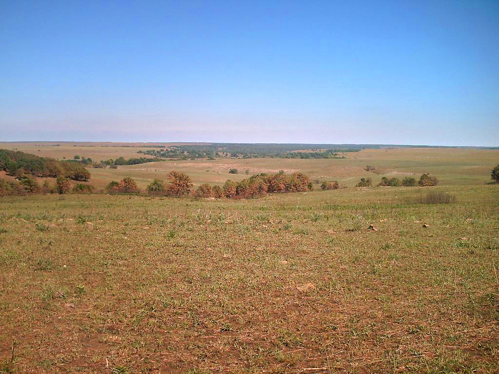
The decreasing patch and core area size and increasing edge and IJI were thought to have major implications for the conservation of grassland vegetation. Many of the grassland biota are sensitive to the minimum core area and the presence of nearby woodland vegetation. The expanding woodlands exacerbated the human‐caused influences on grassland fragmentation. The preservation of the remaining areas of native grasslands is a major conservation effort in the Great Plains of North America (Figure 8.10).

Figure 8.10 The Tallgrass Prairie Preserve, in Osage County, Oklahoma, is protected and managed by Nature Conservancy as the largest tract of remaining tallgrass prairie in the world.
Source: https://upload.wikimedia.org/wikipedia/commons/e/e6/Tallgrass_Prairie_Preserve.jpg.
In a study in the Great Basin of western USA, where the woodland development was more advanced, Bunting and others13 noted a decrease in IJI as woodland vegetation developed. The IJI decreased as smaller and mid‐sized woodland patches coalesced into larger patches of older juniper‐dominated woodland. They also noted that these changes threatened the biota of the nearby nonwoodland vegetation.
Different indices reveal different characteristics of landscape configuration. In this chapter we demonstrated how some of the most common indices are calculated and how they are interrelated. We also saw how configuration indices complement composition indices in the assessment of landscape patterns. These indices all refer to landscapes as they are at a specific moment in time. The dynamic nature of landscapes will be considered in the following chapter.
Key Points
- Landscape patterns are important for understanding landscape processes. Landscape patterns can be described by composition and configuration.
- The composition of a landscape is generally measured by different diversity indices. The simplest measure of landscape composition is richness, the number of habitats present in the landscape. Other diversity indices take into account the proportions of the different habitats.
- Landscape diversity is high when landscape classes become equally abundant while landscape diversity is low when one class becomes dominant in the landscape. Landscape evenness, another measure of landscape composition, can be computed by dividing landscape diversity with its richness.
- Landscape configuration describes the arrangement of patches in the landscape. The simplest configuration metrics describe patch size, number of patches, perimeter, and shape. Shape metrics are generally computed as a ratio of perimeter to area.
- Edge contrast metrics differentiate between different types of edge, accounting for the adjacency of different patch types.
- Configuration can be quantified by cell or patch adjacency. These metrics describe the diversity or evenness of edge types. One common index for describing edge type evenness between patches is the interspersion and juxtaposition index (IJI). IJI is high when patches are interspersed, that is, patch types are likely to neighbor all other patch types in the landscape.
- Contagion is a measure of cell adjacency. Contagion is high when cells of the same type are neighboring each other and decreases when cell type interspersion increases.
- Landscape composition and configuration are important for species occupancy and landscape pattern analysis can assist in the understanding of a species habitat needs. Some species prefer large interior patches while others occupy edges or more fragmented landscapes.