7

CONTROL-SYSTEM DESIGN EXAMPLES: COMPLETE CASE STUDIES

7.1. INTRODUCTION

In the preceding chapters of this book, we have analyzed and designed control systems from specific viewpoints. For example, the Nyquist and Bode diagrams and the root-locus method were applied to linear control systems in Chapter 1, and Chapters 2 and 3, and extended to digital control systems in Chapter 4. The describing function, phase-plane, circle criterion, Liapunov's and Popov's methods were applied to the analysis and design of nonlinear control systems in Chapter 5. How do we take a global viewpoint of a control-system design problem and look at it from both linear and nonlinear viewpoints? We must also consider reliability, cost size, weight, and power consumption. We must design a working control system that meets all the specifications, that can be sold at a profit, that can be built on schedule, and that satisfies the customer's requirements.

In this chapter on complete case studies, we will employ the methods of the preceding chapters to design the following:

1. Design for the positioning system of a tracking radar which illustrates both linear and nonlinear design considerations jointly.
2. Design of the angular control system for a robot's joint.
3. State-variable design for the controller and full-order estimator for a space satellite.
4. Digital control system design for a microcomputer-controlled temperature control system.
5. Robust control system design for controlling the flaps of a hydrofoil.

These examples will illustrate the use of the appropriate methods presented in the book which are needed to design the control system for the intended applications. The design examples will convey the overall approach and methodology used for designing control systems for a good cross section of applications.

7.2. OUTLINE OF PROCEDURE FOR DESIGNING A CONTROL SYSTEM [1, 2]

Due to the availability of a large number of techniques to solve the great variety of control-system problems present, the element of experience is very important to the approach used for the solution of a specific problem. Assuming that the control-system engineer has had some experience with the techniques described, then by logically considering the problem, the many methods described previously in this book provide a very powerful capability. An outline of a logical step-by-step procedure for designing a control system from its conception through the final hardware stage is illustrated in Figure 7.1 and described as follows:

1. Obtain a complete understanding of the job requirements with respect to
   1. a general description of the problem;
   2. the overall control-system performance and accuracy with respect to the steady-state and transient phases;
   3. identification of the transfer function of the controlled process;
   4. miscellaneous requirements as to reliability, schedule, cost, maintainability, size, weight, and available power.
2. Consider several alternative solutions, including electric and hydraulic power servo drives (see Sections 3.4^‡ and 3.5^‡, respectively), the use of continuous control or digital control, etc.
3. Choose the most desired approach based on the specifications, requirements, and elements fixed by the customer.
4. Interpret these requirements in terms of such closed-loop design characteristics as frequency and transient response.
5. Establish the approximate open-loop characteristics that will satisfy the closed-loop requirements.
6. Design the system and select the sensors, actuators, amplifier, and stabilization required (analog or digital) in order to satisfy step 5.
7. Review, refine, and simplify steps 5 and 6.
8. Simulate the system on a computer, including its linear and nonlinear characteristics, to check the design. Make any necessary changes to the design.
9. Build a prototype, and check the design experimentally. Make any necessary changes to the design.
10. Refine the design in order to optimize performance and minimize cost.

Observe from this approach that the procedure is an iterative one, and is itself a feedback process, as illustrated in Figure 7.1

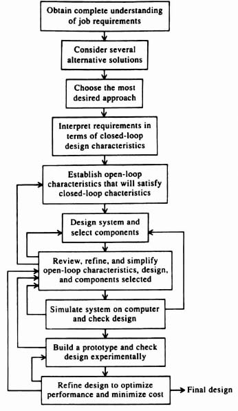
Figure 7.1 Procedure for designing a control system.

7.3. EXAMPLE 1: DESIGN FOR THE POSITIONING SYSTEM OF A TRACKING RADAR USING LINEAR AND NONLINEAR TECHNIQUES JOINTLY [1]

For our first case study, we will design the positioning system of a tracking radar using conventional linear and nonlinear techniques jointly. The demand for precise and smooth positioning of large loads, such as that of a tracking radar, has placed increased emphasis on synthesizing optimum positioning configurations. For example, low resonant frequencies, nonlinear friction, and large opposing wind torques are major problems associated with tracking radars using rotatable antennas (as opposed to tracking radars using electronic scanning) and other positioning systems [1, 3, 4].

Large antennas and associated supporting structures present obstacles to the design of an accurate and smooth tracker. Large masses associated with the load result in relatively low mechanical resonant frequencies, excessive frictional nonlinearities in the form of both Coulomb and static friction (see Section 5.8), and large opposing wind torques. The low resonant frequencies of the tracker necessitate low bandwidths and correspondingly small gain constants that adversely affect accuracy. In addition, the low mechanical resonant frequencies and nonlinear friction can also cause system instability. Assuming that a radome (sheltering structure for a radar antenna) is not used, the large opposing wind torques adversely affect accuracy and require high-power servo ratings. A radome may be undesirable for some applications because of its cost and resulting bore sight shift.

For this application, we will assume that the structural resonance has its first peaking at 4 Hz of 13 dB, and there are higher resonance peaks at greater frequencies. The allowable resonances are shown on the Bode diagram in Figure 7.2. This type of structural resonance limits the dynamic accuracy of the friction-stabilization inner loop and, consequently, the auto-track outer loop. Assuming a minimum gain margin of 6 dB and a structural resonance peaking of 13 dB at 4 Hz, a system containing two pure integrations in the auto-track loop could result in an acceleration constant K_a equal to 1, as shown in Figure 7.2. This is insufficient for our design. Therefore, we want to go to an auto-track loop that has three pure integrations and provides for an infinite K_a.

In addition, we will assume that this tracking system must contend with three forms of friction. These are viscous, Coulomb, and static friction (stiction), which were analyzed in Section 5.8 from the describing-function method. We will analyze the effect of Coulomb and static friction on the system from a nonlinear, describing function viewpoint.

Let us consider the possibility of using N pure integrations in the auto-tracking loop to track d^N–1 θ/dt^N–1 dynamics perfectly, and to overcome the structural resonance limitation [3, 4]. Conventional linear theory indicates that it is feasible to stabilize a positioning loop containing N pure integrations, where N can be equal to or greater than 3. These techniques also illustrate that the use of these systems in the presence of multiple nonlinearities does present nonlinear stability problems that must be solved. Let us examine the effects of five different auto-tracking loop types ranging from type 0 (contains zero pure integrations) to type-4 (contains four pure integrations) on the overall tracking-system stability and accuracy when operating in the presence of multiple frictional nonlinearities. A comprehensive analysis is performed on a single-loop tracking configuration and then extend to the case of the multiple-feedback loop. The concept is then extended to the design of a practical tracking radar system employing three pure integrations (type 3) in the auto-track loop. The tracking system, which is also analyzed from a nonlinear viewpoint, exhibits velocity and acceleration constants of infinity and, therefore, easily solves the accuracy problem introduced by low resonant frequencies. In addition, a highly damped rate-feedback loop further isolates the frictional nonlinearities, thereby preventing limit cycles due to nonlinear friction. It is shown that the practical tracking configuration utilizing multiple-feedback loops is completely stable from both a linear and nonlinear viewpoint, and exhibits very high accuracy.

Figure 7.2 The resonance problem in a tracking radar using a rotatable antenna.

To evaluate the effect of system type (the number of pure integrations in the positioning auto-track loop), consider the simple one-loop configuration containing a nonlinear element in Figure 7.3. Assuming that H(s) = 1, then Figure 7.4 shows how a positioning loop can be designed containing zero (type 0) to four pure integrations (type 4) in which the system is stable. All the systems have a 65° phase margin from purely linear considerations. Bode's first weighting-function theorem verifies the linear stabilization of type-N configurations (see Section 2.6).

To completely determine the stability of type-n positioning (tracking) loops, it is also necessary to analyze the system from a nonlinear viewpoint. All practical tracking and positioning systems must contend with the realistic nonlinear characteristics of Coulomb friction and stiction (see Section 5.8).

The characteristic equation of the single-loop configuration of Figure 7.4 can be written in the form of Eq. (7.1), from which stability can be readily determined:

In this equation, G(jω)H(jω) represents the linear portion of the loop gain and N(M, ω) represents the describing function of the nonlinearity as a function of its input signal amplitude M and frequency ω. From Eq. (5.81), the criterion for nonlinear instability of the single-loop configuration is given by

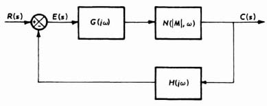
Figure 7.3 General nonlinear system.

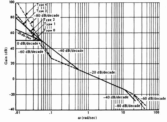
Figure 7.4 Bode diagrams of linearly stable type 0 through type 4 configurations.

The gain-phase diagram will be used to perform this describing-function analysis as described in Sections 5.7–5.12. The describing function for the combined case of Coulomb friction and stiction [see Eq. (5.75)] has been used for analysis shown in Figure 7.5, where the effect of this combined nonlinearity on positioning loops having the type 0 through type 4 configurations illustrated in Figure 7.5 are shown. It is concluded that type 0, type 1, and type 2 single-loop configurations containing nonlinear friction are completely stable from nonlinear considerations. However, the type 3 and type 4 single-loop configurations are shown to exhibit limit cycles. The type 4 configuration clearly shows an intersection on the gain-phase diagram, whereas the type 3 configuration loci approach the describing-function loci at very low frequencies. However, the margin of stability of the type 3 system is negligible at moderate frequencies and borders on instability. Thus, for all practical purposes, it must be considered unstable.

Although single-loop systems greater than type 2 are unstable in single-loop configurations because of frictional nonlinearities, multiple-feedback loops can improve the situation. Therefore, the synthesis of a type 3 system using multiple loops, which is stable from both linear and nonlinear considerations, is described in this design.

Figure 7.5 Describing-function analysis of type 0 through type 4 conligurations.

The key to the successful synthesis of high-order systems is the proper design of the inner feedback loops. Great care must be exercised in isolating the nonlinear elements by a very heavily damped inner loop or loops. As an example of this approach, a type 3 tracking positioning system will be designed that contains the nonlinear frictional characteristics of Coulomb friction and stiction.

The basic multiple-loop configuration can be constructed around an analysis using describing-function and signal-flow graphs (see Sections 2.14–2.16^‡). A method of accomplishing the design is illustrated with the aid of Figure 7.6, and the corresponding signal-flow graph is shown in Figure 7.7. Using Mason's theorem, given Eq. (2.135)^‡, the overall system transfer function is given by Eq. (7.3).

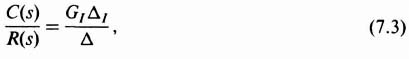
Figure 7.6 Representative multiple-feedback control system containing a nonlinearity common to all feedback paths.

Figure 7.7 Signal-flow diagram for system shown in Figure 7.6.

where

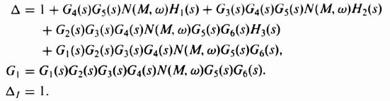
Therefore,

Stability for this system can be determined from the zeros of the characteristic equation:

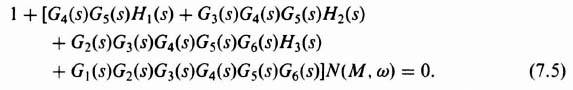
From this step, stability can then be determined using the gain-phase diagram.

For the particular problem of a tracking radar containing a rotatable antenna, the general configuration in Fig. 6.6 applies. Therefore, we now have a technique readily applicable to the analysis of nonlinearities in a type 3 multiple-feedback system. The particular configuration to which this method will be applied consists of a tracking radar that uses a Ward-Leonard power drive system (see Section 3.4^‡), having armature current and field current feedback to decrease the armature and field time constants (see Problem 3.7^‡).

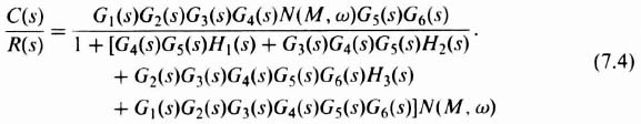
Figure 7.8 illustrates the equivalent configuration of the tracking radar control system. Notice that the hypothetical system considered in Figure 7.6 corresponds to the proposed structure. Therefore, the system stability can be studied from a gain-phase plot of Eq. (7.5). The values for G₄(s), G₅(s), G₆(s), H₁(s), H₂(s), and H₃(s) are dictated by practical considerations. It remains for the control-systems engineer to choose G₁(s), G₂(s) and G₃(s).

The primary function of the rate feedback, H₃(s), is to prevent oscillations due to the nonlinear friction characteristics of stiction and Coulomb friction. It is designed specifically with a very high damping ratio to overcome this problem.

The describing function analysis of this type 3 system is illustrated in Figure 7.9, which considers the case where Coulomb fraction F_c and stiction F, are both present. It is extremely important for the control system to remain stable when the tracking loop is open and closed. When the tracking loop is open, the radar-system tracking is interrupted. This condition can be shown by removing G₁(s) and its corresponding feedback path in Figure 7.8.

The values for G₂(s) and G₃(s) are dictated primarily from nonlinear considerations as shown on the gain-phase diagrams of Figure 7.9, while the value of G₁(s) is dictated primarily from linear considerations as shown on the Bode diagram of Figure 7.10. However, there is some interdependence, and a trial-and-error solution is required. The resultant gain-phase diagram of Figure 7.9 in conjunction with the Bode diagram of Figure 7.10 indicate that the system is completely stable from a linear and nonlinear viewpoint when

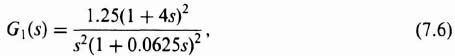
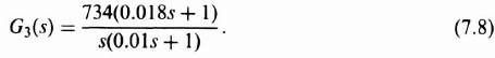
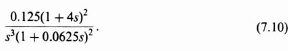
The open-loop transfer function for the Bode diagram of Figure 7.10 was obtained by assuming that the gain of the inner loop containing H₃(s) as feedback in Figure 7.8 has a high gain over the frequencies of interest and, therefore, the auto-track loop sees its transfer function as [see Eq. (2.122)^‡]

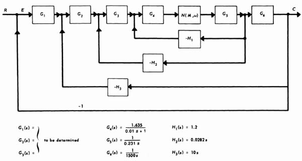
Figure 7.8 Equivalent representation of the tracking radar control system.

Figure 7.9 Describing-function analysis for Coulomb friction and static friction [1].

Therefore, the open-loop transfer function of the auto-track loop is given by

This design has resulted in a type 3 ninth-order practical system that has zero steady-state error resulting from inputs of position, velocity, and acceleration.

Figure 7.10 Tracking loop: open-loop frequency characteristics [1].

It is important to recognize that although this design problem focused on positioning a tracking radar containing a rotatable antenna, the approach is equally valid for the positioning control problem of any large load containing nonlinear friction.

7.4. EXAMPLE 2: DESIGN OF AN ANGULAR CONTROL SYSTEM FOR A ROBOT'S JOINT

Robots are playing an increasingly important role in manufacturing and other applications. Figure 7.11 shows an example of the use of robots to manufacture automobiles at the Ford Motor Company where a robot is used to automatically mate a hood inner panel to the outer panel for a Ford Taurus at its Woodhaven (MI) Stamping Plant.

For the second design example, the angular control system of a robot's joint will be designed. The specifications for this application are as follows:

1. steady-state error due to a velocity input of 3.2 rad/sec should equal or be less than 0.1 rad; steady-state error of zero due to position inputs;
2. phase margin greater than 60°;
3. settling time of less than 1 sec;
4. percent overshoot of less than 8%.

Figure 7.11 Robot being used to automatically mate a hood inner panel to the outer panel for a Ford Taurus at Ford Motor Company's Woodhaven (MI) Stamping Plant. (Courtesy of the Ford Molor Company)

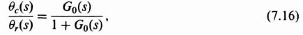
The block diagram for controlling the robot's joint is illustrated in Figure 7.12, It will be assumed that the transfer function θ_c(s)/E_A(s) in this problem can be approximated by*

Because this transfer function has one pure integration, the specification requirement of zero steady-state error due to position inputs will be met (see Appendix C), Nonlinearities in this control system are assumed to be negligible,

As the first step in the design, the value of the amplifier gain K_A to satisfy the steady-state accuracy will be obtained, Assuming that G(s) = 1 for this part of the analysis, the forward function θ_c(s)/E(s) is found to be

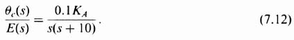
Figure 7.12 Block diagram for controlling a robot's joint,

From the specifications, the value of the desired velocity constant K_ν is given by

Therefore, the value of the amplifier gain K_A is given by (assuming G_c(s) = 1) and

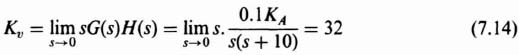
and

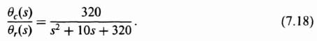
With this value of amplifier gain and without any compensation, G_c(s), the phase margin, percent overshoot, and settling time will be determined. The closed-loop transfer function of this second-order system is given by

where

Therefore,

Using Eq. (B.2), the undamped natural frequency ω_n and damping ratio ζ are found to be

From Eq. (B.33), the maximum percent overshot for ζ = 0.28 is 40.01%, much higher than the specification maximum of 8%. From Eq. (5.41)^‡, the settling time for ζ = 0.28 is 0.798 sec and is within the specification value of 1 sec. The Bode diagram of this uncompensated system is illustrated in Figures 7.13a and b, and shows a phase shift of −148.9° at gain crossover frequency and a phase margin of only 31.10, which is much less than the specified phase margin of 60° minimum. Figures 7.13a and b were obtained using MATLAB (see Section 1.7) and contained in the M-file which is part of the Advanced Modern Control System Theory and Design (AMCSTD) Toolbox and can be retrieved free from The MathWorks, Inc. anonymous FTP server at ftp://ftp.mathworths.com/pub/books/advshinners. Therefore, we must compensate this system to meet the specifications.

Figure 7.13 Bode diagram of uncompensated control system for robot.

A phase-lead or phase-lag network can be selected for the design based on the specifications. However, from the tradeoffs between the two networks discussed in Section 2.10, a phase-lag network is selected, because it is less expensive (an increase in the amplifier gain is needed with a phase-lead network due to its de attenuation), provides the compensated system with a smaller bandwidth and, therefore, the resulting system has less noise and the output response has less “jitter.”

Using the approach discussed in Section 2.6, the following phase-lag network was selected:

Therefore, the open-loop transfer function is obtained from Eqs. (7.17) and (7.21) to be

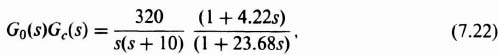
and its Bode diagram is drawn in Figures 7.14a and b. These figures were obtained using MATLAB (see Section 1.7) and are also contained in the M-file which is part of the AMCSTD Toolbox. The phase shift at gain crossover frequency of the compensated system is −119.2°, with a resulting phase margin of 60.8°, and this satisfies the specification on phase margin (60° minimum).

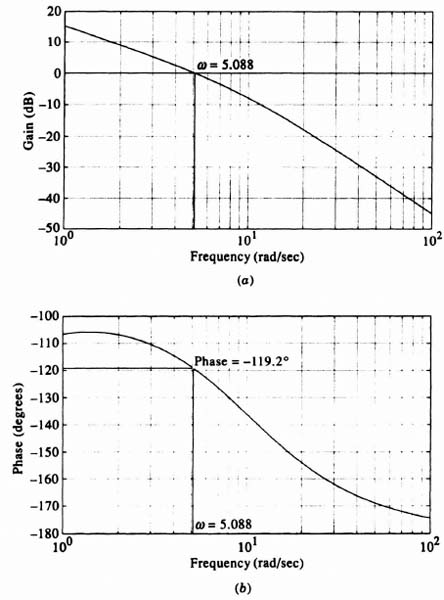
Figure 7.14 Bode diagram of compensated control system for robot.

Having met the stability and accuracy specification of the design, the resulting transient response must be checked. The closed-loop transfer function of the compensated system is

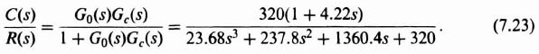
Factoring the denominator, we obtain

Thus, the dominant pair of complex-conjugate roots are given by s = −4.90 ± j5.57. As shown in Figure B.3, the corresponding value of ω_n is given by 7.42. Therefore, the value of the damping ratio ζ for the compensated system can be obtained from Eq. (8.18) as

Therefore,

Note that the damping ratio of the uncompensated system was 0.28 [see Eq. (7.20)]. From Eq. (8.33), the maximum percent overshoot for the compensated system for a damping ratio of 0.66 is reduced to 6.33%, and this satisfies the specification that it be less than 8 percent. From Eq. (5.41)^‡, the settling time of the compensated system for a damping ratio of 0.66 is 0.82 sec, and this also satisfies the specification that it be less than 1 sec.

In conclusion, the phase-lag network of Eq. (7.21) in conjunction with the amplifier gain given by Eq. (7.15) meet all of the steady-state error, stability, and transient specifications for this design. Table 7.1 summarizes the specification requirements, and the uncompensated and compensated values for these parameters.

Table 7.1. Comparison of Design Parameters for Specification, Uncompensated System and Compensated System

7.5. EXAMPLE 3: DESIGN OF THE CONTROLLER AND FULL-ORDER ESTIMATOR FOR A SPACE SATELLITE'S ATTITUDE-CONTROL SYSTEM WITH POLE PLACEMENT USING LINEAR-STATE-VARIABLE FEEDBACK

For the third design example, the controller and full-order estimator of a satellite's attitude control system will be designed with pole placement using linear-state-variable feedback.

The attitude-control problem is illustrated in Figure 7.15. The satellite is assumed to be rigid, operating in a frictionless environment, and disturbing forces are negligible. It is desired that the angle θ(t) be zero. However, the satellite will drift with time, and jets aboard the satellite will be fired so that θ(t) is driven to zero. The dynamics of the system are similar to the space attitude-control problem analyzed in Section 6.6. Assuming that the torque T(t) due to the jet firings is the input to the system and the attitude angle θ(t) is the output, then the differential equation relating input and output is given by

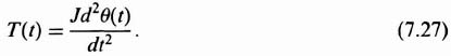
By defining

then Eq. (7.27) can be written as

Using dot notation, Eq. (7.29) simplifies to

The design specifications for this attitude-control system are as follows:

1. The system's controller must be critically damped.
2. The settling time of the system's controller must be 1 sec or less.

   

   Figure 7.15 Control of space satellite's attitude.

3. The estimator must also be critically damped, an it must be two and one half times faster than the controller (e.g., ).

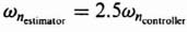The controller will be assumed to have the following form:

where u(t) is the input torque, x₁(t) is the attitude angle, and x₂(t) is the attitude velocity.

The form of the controller's closed-loop transfer function is given by

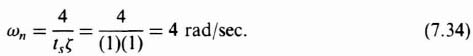
The value of ω_n can be determined by substituting the specification values of critical damping (ζ = 1) and settling time (t_s) of 1 sec into Eq. (5.41)^‡:

Solving for ω_m

Therefore, the numerator and denominator's constant of Eq. (7.32) are given by

and Eq. (7.32) can be written as

The resulting characteristic equation of this system is given by

To find the controller gain K, Eq. (3.167) will be used:

The state-equation representation of Eq. (7.30) is given by

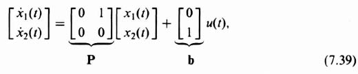
Substituting the values of P and b from Eq. (7.39) into Eq. (7.38), the following is obtained:

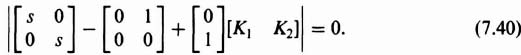
This simplifies to

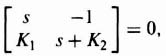
from which we obtain the characteristic equation of the controller:

Comparing like coefficients in Eqs. (7.37) and (7.41), solutions of K₁ = 16 and K₂ = 8 are obtained. Therefore,

and the controller's characteristic equation is given by

The controller is given by

which is the form of the controller specified [see Eq. (7.31)].

For the next part of the design, the full-order estimator will be designed. Because the estimator is specified to be 2.5 times faster than the controller,

Because

The estimator is specified to be critically damped. Therefore, the characteristic equation of the estimator is given by

To find the estimator, Eq. (8.173) will be used:

Substituting for P and L from Eq. (7.39) into Eq. (7.48), the following is obtained:

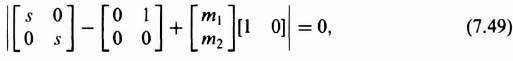
which reduces to

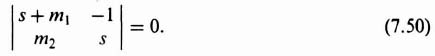
The resulting characteristic equation of the estimator in terns of m₁ and m₂ is given by

Setting like coefficients in Eqs. (7.47) and (7.51) equal to each other, the following is obtained: m₁ = 20; m₂ = 100. Therefore,

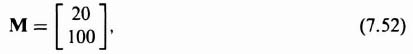
and the characteristic equation of the estimator is given by

Having designed the controller and estimator, the transfer function of the compensator will next be determined from Eq. (3.162) and Figure 3.19:

Substituting Eqs. (7.39), (7.42), and (7.52) into Eq. (7.54), the following is obtained:

This reduces to

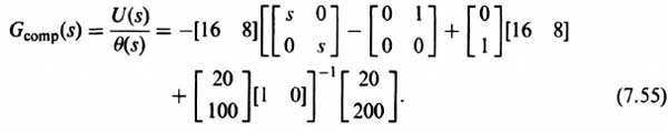
The inverse matrix portion of Eq. (7.56) is given by

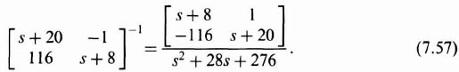
Substitution of Eq. (7.57) into (7.56) results in the following:

Factoring the denominator, the following transfer function is obtained:

The transfer function of the satellite can be represented by [see Eq. (7.30)]

Therefore, the open-loop transfer function of the complete system is given by

To check the resulting design, the root locus and Bode diagram will be used. For the root-locus design, the specific gain will be replaced with the variable gain K:

which is shown in Figure 7.16. Observe that the root locus goes through the roots selected in Eqs. (7.43) and (7.53). These roots are shown in Figure 7.16 by asterisks. Note that K = 1120 at these roots. This figure was obtained using MATLAB (see Section 1.7), and is contained in the M-file which is part of the AMCSTD Toolbox and can be retrieved free from The MathWorks. Inc. anonymous FTP server at ftp://ftp.mathworks.com/pub/books/advshinners.

To draw the Bode diagram, the modified form of Eq. (7.62) is analyzed:

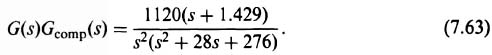
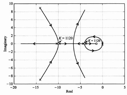
Figure 7.16 Root locus for compensated attitude-control system.

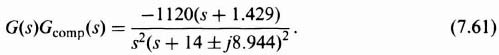
The resulting Bode diagram is drawn from the following modification to Eq. (7.63):

The quadratic poles in the denominator have a natural resonance frequency ω_n and a damping ratio ζ given by

The resulting Bode diagram is shown in Figure 7.17. This figure was obtained using MATLAB (see Section 1.7), and is also contained in the M-file which is part of the AMCSTD Toolbox.

It is concluded that the uncompensated transfer function.

has its phase margin increased from 0° to 46.78° (measured at gain crossover frequency of 4.174 rad/sec), and its gain margin is increased from −∞ to 15.41 dB (measured at the phase crossover frequency of 15.36 rad/sec) for the compensator of Eq. (7.59). Notice that the gain crossover frequency of 4.174 rad/sec is approximately consistent with the controller's closed-loop roots of ω_n = 4 and ζ = 1. This is a reasonable result, as the slower roots of the controller are more dominant than the faster estimator roots on the system response.

Figure 7.17 Bode diagram of compensated attitude-control system.

7.6. EXAMPLE 4: DESIGN OF A SAMPLED-DATA CONTROL SYSTEM FOR CONTROLLING THE TEMPERATURE OF A LIQUID IN A TANK

For the fourth design example in this chapter, the closed-loop temperature digital control system illustrated in Figure 7.18a will be designed. The microcomputer output controls the position of a solenoid valve, which then controls the quantity of steam into the tank coil. Feedback is obtained from a thermocouple in the tank, whose signal is amplified and then converted to a digital signal, for use by the microcomputer. In this manner, the microcomputer controls the temperature of the liquid contained in the tank in a closed-loop manner. The resulting block diagram of this thermal control system is illustrated in Figure 7.18b. The microcornputer will be represented by D(z), the zero-order hold by G_H(s), and the transfer function of the thermal process for heating the liquid in the tank is given by [5]

Figure 7.18 Temperature control system. (From Phillips and Nagle (5). (Reprinted by permission of Prentice-Hall, Englewood Cliffs, NJ)

Observe that the transfer function of the thermal process G_p(s) is of the same form as derived in Section 3.6^‡, Eq. (3.152^‡), for heating water in a tank.

The specifications for this design problem are as follows:

1. The steady-state error for a step input of 10°C temperature should be less than or equal to 2%.
2. The system should have a minimum phase margin of 60°.
3. The sampling time is 0.5 sec.

The design problem is to determine the value of D(z) to meet these specifications.

The system will first be analyzed without any compensation [D(z) = 1]. The closed-loop transfer function of the uncompensated system is given by the following:

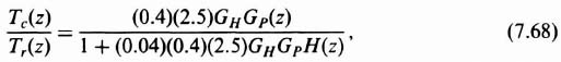
where T_r(z) and T_c(z) represent the z transform of the desired input and actual output temperature, respectively, and

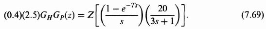
For the T = 0.5 sec, this reduces to the following:

In addition, the feedback sensor's transfer function H(z) = 0.04. Therefore,

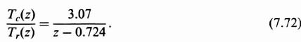
Substituting Eqs. (7.70) and (7.71) into Eq. (7.68), the following closed-loop transfer function is obtained:

For a step input of 10°C,

The output response is obtained by substituting Eq. (7.73) into (7.72):

Simplifying Eq. (7.74), the following is obtained:

In terms of negative powers of z,

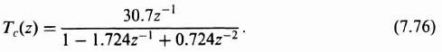
To find the time-domain solution, the denominator of Eq. (7.76) is divided into its numerator and the following series is obtained:

Taking the inverse z transform of Eq. (7.77), the following series is obtained in the discrete-time domain:

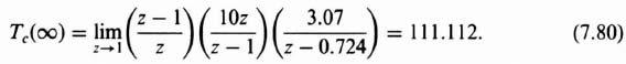
The result is plotted in Figure 7.19 for terms taken out to 100 sec. From this plot, it is seen that the system is very overdamped and slow. It takes approximately 15 sec to reach its steady-state value of 111.112. To find the steady-state value, the final-value theorem of Eq. (4.61) will be applied to Eq. (7.74):

Substituting Eq. (7.74) into Eq. (7.79), the following equation is obtained for the steady-state value:

The percent steady-state error for a step input of 10°C can be determined from

Substituting Eq. (7.71) and

Figure 7.19 Transient response of uncompensated temperature control system.

into Eq. (7.81), the following is obtained:

Therefore, applying the final-value theorem of Eq. (4.61) to Eq. (7.83), the following is obtained:

This reduces to

Therefore, the steady-state error for the step input of 10 e is 55.5% which greatly exceeds the specification level of 2%. From the transient response of Figure 7.19, the final value of 111.112 is in error by 55.5% of the expected value of 250 (which is the reciprocal of the feedback transfer function of 0.04 times the 10° step input of temperature, or 250).

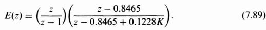
In the next stage of the design, the value of K will be determined, which results in a 2% error to a step input which is a specification requirement. With D(z) = K, the value of K can be determined as follows:

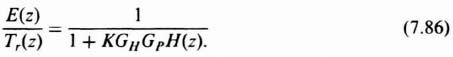
Substituting Eq. (7.71) into Eq. (7.86), the following is obtained:

For a unit step input of temperature,

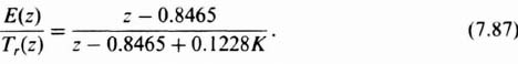
Substituting Eq. (7.88) into Eq. (7.87), the following expression for error is obtained:

To satisfy a 2% steady-state error requirement for a unit step input, the final-value theorem is applied to Eq. (7.89) as follows (note that the percent error is the same for any constant input with T = 0.5 sec):

Solving for K.

Therefore, a gain of D(z) = K = 61.25 is needed to keep the steady-state error at 2%. It is interesting to analyze the stability of this system with D(z) = K = 61.25. The closed-loop transfer function is given by

Substituting Eq. (7.71) into Eq. (7.92), the following is obtained:

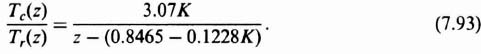
With K = 61.25, this simplifies to

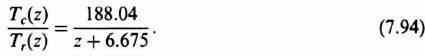
Note that the characteristic equation obtained from Eq. (7.94) is given by

and indicates a root outside the unit circle at −6.675 in the z-plane. Therefore, this incompensated system will be unstable.

A digital controller will next be designed which has K = 61.25 and contains compensation to satisfy the specification requirements of a minimum phase margin of 60°. The open-loop transfer function of the system with K = 61.25 is given by [see Eq. (7.71)]

Transforming Eq. (7.95) into the w-plane, we use Eq. (4.175),

Substituting Eq. (7.96) with T = 0.5 sec into Eq. (7.95), the following is obtained:

To compensate the system, a zero will be added to cancel the pole term in Eq. (7.97). To achieve the desired phase margin, a pole term (1 + ω/0.039), was added as follows:

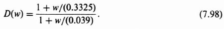
Therefore, the open-loop transfer function of the compensated system is obtained by multiplying Eqs. (7.97) and (7.98). The result is as follows:

Figure 7.20 shows a Bode diagram of the compensated system, which has a phase margin of 62.32° and an infinite gain margin. Therefore, the specification on stability has been achieved. This Bode diagram was drawn using MATLAB (see Section 1.7), and is contained in the M-file that is part of the AMCSTD Toolbox which can be retrieved by the reader free from The MathWorks, Inc. anonymous FTP server at ftp://ftp.mathworks.com/pub/books/advshinners.

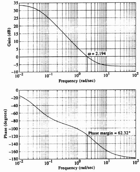
Figure 7.20 Bode diagram of compensated temperature control system.

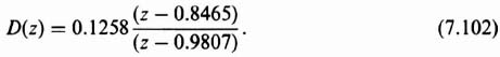
The compensating network of Eq. (7.98) will be converted back into the z plane using Eq. (4.167):

Because T = 0.5 sec, this reduces to

Substituting Eq. (7.101) into Eq. (7.98), the following is obtained:

Incorporating the gain of K = 61.25 [see Eq. (7.91) into the digital controller, the total transfer function of the digital controller is given by

which reduces to

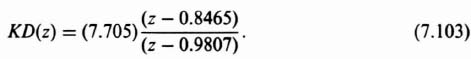
Therefore, the open-loop transfer function of the temperature control system can be obtained from Eq. (7.71) and (7.103) as follows:

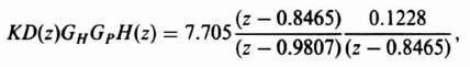
which reduces to

The steady-state error of the resulting compensated system can be checked to determine that it meets the steady-state error specification as follows:

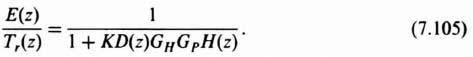
Substituting Eqs. (7.88) and (7.104) into Eq. (7.105), the following is obtained:

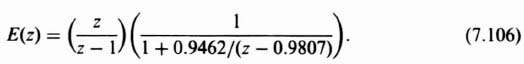
Applying the final-value theorem to Eq. (7.106)

Therefore, the compensated system has a 2% steady-state error to a unit step input, and satisfies the specification requirement on steady-state error.

To complete the design, the transient response of the compensated system will be determined. The closed-loop transfer function of the compensated system is given by

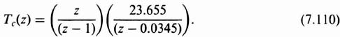
Substituting Eq. (7.104) into Eq. (7.108) and accounting for the fact that H(z) = 0.04, the following is obtained:

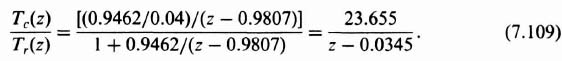
Substituting a unit step input of temperature (the transient response can be determined using a unit step as well as an input of 10°C) for T_r(z) in Eq. (7.109), the following expression of the output temperature is obtained:

From the following expression,

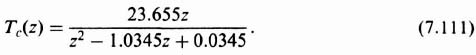
T_c(z)'s series output is obtained by dividing denominator into numerator:

In the time domain, this series is given by

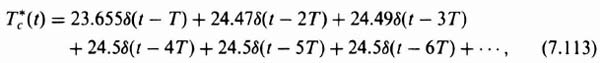
where T = 0.5sec. The result is shown in Figure 7.21. From this graph, it can be seen that the system's respon se has improved dramatically compared to that of the uncompensated system shown in Figure 7.19. In approximately 2 sec, the system reaches its steady-state value of 24.5. This results in a 2% error with the ideal value of 25 (unit input divided by the feedback element's transfer function of 0.04).

In conclusion, this design has achieved all of its design specifications. The uncompensated system was stable, but it had a very large steady error and was very sluggish. Increasing its gain to meet the steady-state accuracy requirement made the system unstable. By compensating it with the digital controller, it was stabilized, met its accuracy requirements, and its transient response was greatly improved.

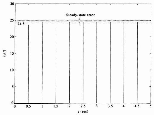
Figure 7.21 Transient response of compensated temperature control system.

7.7. EXAMPLE 5: DESIGN OF A ROBUST CONTROL SYSTEM FOR CONTROLLING THE FLAPS OF A HYDROFOIL [6–10]

In the fifth design example in this chapter, we wish to control the flaps of a hydrofoil. Consider the conceptual illustration in Figure 7.22 which illustrates sea waves hitting the flaps of the hydrofoil. This causes large resultant torques that try to turn the flaps from their desirable positions. These torques can be viewed as the torque disturbances D(S) illustrated in the equivalent block diagram of the two-degrees-of-freedom robust control system for controlling the angular flap position shown in Figure 7.23. In the real world, sea waves and their resultant torque are a stochastic process. However, we will assume in this design example that the torque disturbances due to sea waves can be averaged for the environment in which the hydrofoil will operate and can be represented deterministically as a unit step input.

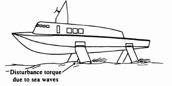
Figure 7.22 A hydrofoil boat illustrating sea waves causing disturbance torques.

We wish to design the robust control system for controlling the angular position of the hydrofoil's flaps as illustrated in Figure 7.23 to minimize the effects of the disturbance torques D(s) and with gain variations from K = 40 to 10 and 100.

The two-degrees-of-freedom control system illustrated in Figure 7.23 was analyzed thoroughly in Section 3.10 in the discussion of robust control systems. It was shown that since the transfer function C(s)/D(s) [given by Eq. (3.198]) and the sensitivity of H(s) with respect to K [given by Eq. (3.201)] are identical, then the same control system techniques can be used to suppress the effect of the disturbance D(s) and achieve robustness (insensitivity) with respect to variations of K. The transfer function of the hydrofoil dynamics will be assumed in this case study to be given by the following transfer function:

We will first assume that G_c1(s) = G_c2(s) = 1, and we will investigate the effect of the variation of K where K = 10, 40, and 100. Therefore,

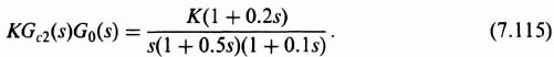
Figure 7.24 illustrates the unit step response of the system when K = 10, 40, and 100. Table 7.2 lists the damping ratio of the unit step transient responses and the characteristic equation roots of this control system which were obtained using MATLAB. Observe that the variations in K = 10, 40, and 100 result in considerable variation in the transient responses of this control system. Figure 7.25 illustrates the root loci and location of the closed-loop, complex-conjugate roots of the cases being analyzed.

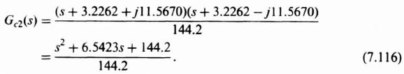
As discussed in Section 3.10, the design approach for this robust controller, G_c2(s), is to place two zeros at (or near) the desired complex-conjugate loop poles at −3.2262 ± j11.5670 for the nominal gain case of 40. Therefore,

Figure 7.23 The equivalent block diagram for control of the hydroloil boat of Figure 7.22 using a two-degrees-of-freedom robust controller.

Figure 7.24 Unit step response of Figure 7.23 with KG_c2(s)G₀(s) give n by Eq. (7.115) and G_c1(s) = 1.

Table 7.2. Characteristics of the Control System Illustrated in Figure 7.23 where KG_c2(s)G₀(s) is given by Eq. (7.115) and G_c1(s) = 1

Figure 7.25 Root-locus for system of Figure 7.23 with KG_c2(s)G₀(s) given by Eq. (7.115) and G_c1(s) = 1.

The forward-path transfer function of this control system with KG₀(s) given by Eq. (7.115) and G_c2(s) given by Eq. (7.116) is:

Table 7.3 lists the characteristics of the damping ratio and the characteristic equation roots of this control system, obtained using MATLAB, with the forward-loop transfer function given by Eq. (7.117). Observe that the damping ratios are much closer (0.317 to 0.483) than they were before the addition of the robust controller G_c2(s) as shown in Table 7.2 (where the damping ratio previously varied from 0.173 to 0.431).

Figure 7.26 illustrates the root loci with the robust controller G_c2(s) added, and the location of the closed-loop, complex-conjugate roots for the three cases. Observe from this root locus that by locating the two zeros of the forward-loop controller G_c2(s) near the desired characteristic equation complex-conjugate roots, then the sensitivity of this control system is much better. The result is that the sensitivity of the system as K varies is much better than before.

Table 7.3. Characteristics of the Control System Illustrated in Figure 7.23 with the Forward-Loop Controller G_c2(s) Added and where KG_c2(s)G₀(s) is given by Eq. (7.117)

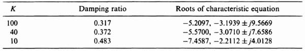
Figure 7.26 Root-locus for system shown in Figure 7.23 with KG_c2(s)G₀(s) given by Eq. (7.117) and G_c1(s) = 1.

As was shown in Section 3.10 on robust control systems, it is necessary to add the series controller G_c1(s) whose transfer function is the reciprocal of that given by G_c2(s):

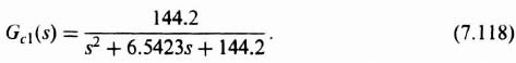
The unit step respon se of this control system with the forward-path transfer function of the control system given by Eq. (7.117), with K = 10, 40, and 100, and with the series controller transfer function given by Eq. (7.118), is illustrated in Figure 7.27. Comparing these unit step responses with those in Figure 7.24, we conclude that this control system has been made to be much less sensitive to variations in K. The maximum percent overshoots to a unit step input ranged from 30% to 61% in Figure 7.24 for the original system, and only 23% to 38% for the robust design in Figure 7.27. In addition, as was pointed out before, the robustness with respect to variations in K will also provide disturbance suppression using the same control techniques as the two-degrees-of-freedom control system shown in Figure 7.23.

Figure 7.27 Unit step response for system of Figure 7.23 with KG_c2(s)G₀(s) given by Eq. (7.117) and G_c1(s) given by E1. (7.118).

PROBLEMS

1. 7.1. We wish to design a hydrofoil ship, which is conceptually illustrated in Figure P7.1a, and whose block diagram is illustrated in Figure P7.1b. As illustrated, sea waves hitting the flaps cause large resultant torques that try to turn the flaps from their desirable positions. In effect, the sea waves can be viewed to be a torque disturbance U_r(s), as shown in Figure P7.1b. Although sea waves and their resultant torque are a stochastic process, we will assume in this problem that the torque disturbance due to sea waves can be averaged for the environment in which this hydrofoil will operate to be a unit step input. The specifications for this hydrofoil control system are that the steady-state error due to a unit step input U_T(s) shall not exceed a steady-state error at E(s) of 0.1 and the stability requirement for the stabilized control system is a minimum phase margin of 50° and a minimum gain margin of 20 dB. In addition, a minimum gain crossover of 8 rad/sec is required to achieve the desired response time.

   

   Figure P7.1 A hydrofoil boat illustrating sea waves causing disturbance torques (a), and its equivalent block diagram (b).

   1. With the compensation network G_c(s) set equal to 1 and K set equal to 1, determine the phase and gain margins of this system.
   2. With the compensation network G_c(s) set equal to 1, determine the gain K required to achieve the steady-state error requirement of 0.1 due to a unit torque disturbance at U_T(s).
   3. With the gain K found in part (b), determine the resulting phase and gain margins of the systems.
   4. Design the compensation network G_c(s) that will achieve the stability requirements.
2. 7.2 It is desired to design the positioning system of the tracking radar illustrated in Figure P7.2a which does not have a radome (sheltering structure for a radar antenna) to prevent wind from causing torque disturbances. It has been shown in Reference 1 that winds having velocities of 50 knots can cause wind torque disturbances of approximately 4000 ft lb on a parabolic reflector of 16 ft in diameter. Wind and wind gust occurrence and its resultant wind torque disturbances on the positioning control system is a stochastic problem. However, for this problem, we will design for an average wind where this radar will be operating. It will be assumed that the average wind can be represented as a step of 10 units. The specifications for the design of this positioning loop require that the steady-state error of E(s) due to a step input of 10 units at U_T(s) should be 1.25. Stability requirements are that the compensated system shall have a minimum phase margin of 50 and a minimum gain margin of 20 dB. In addition, to minimize the effects of tracking jitter caused by noise in the tracking loop, we wish to limit the maximum gain crossover frequency to 1.5 rad/sec.

   

   Figure P7.2 A tracking radar conceptually illustrating disturbance torques due to wind forces (a), and the equivalent block diagram of the tracking radar's positioning loop (b).

   1. With the compensation network G_c(s) in Figure P7.2b, set equal to 1, find the gain K needed to achieve the steady-state error requirement of 1.25 due to the torque step disturbances at U_T(s) of 10 units.
   2. With the value of K found in part (a), draw the Bode diagram of this system and find the resulting phase and gain margins.
   3. Design the compensation network G_c(s) that will achieve the specified phase and gain margins.
   4. Determine the transient response of the uncompensated system of part (b) and the compensated system of part (c) to a unit step input.
3. 7.3. Figure P7.3a shows a conceptual illustration of a robot performing a welding task in the manufacture of an automobile, which is a common application of robots. Suppose it is desired to design the angular positioning system for such a robot. Figure 7.3b illustrates the block diagram of the system. The specifications for the design of this system are that the positioning system have a damping ratio of 0.707, a position constant K_p of infinity, and a velocity constant K_ν equal to 10.

   

   Figure P7.3 A conceptual illustration of a robot performing a welding task in the manufacture of an automobile (a), and an equivalent block diagram of the angular positioning system (b).

   1. With the compensation network G_c(s) set equal to one, draw the root locus of the system.
   2. Find the value of gain K that will result in a damping ratio of 0.707, and indicate it on the root locus.
   3. Find the compensation G_c(s) that will achieve a velocity constant of 10. Draw the resulting root locus.
   4. Find the transient response of the compensated system to a unit step input.
   5. How does the transient response of part (d) compare with the desired damping ratio of 0.707?
4. 7.4. Repeat Problem 7.3 if the desired damping ratio is 0.5 instead of 0.707.
5. 7.5. We wish to design an autopilot for controlling the roll of an airplane. In practice, the following three surfaces of an airplane are controlled in order to achieve the desired attitude of an aircraft: ailerons, elevators, and rudder, as illustrated in Figure P7.5a. The autopilot for controlling the roll of an aircraft can be controlled by adjusting the angle of the aileron's surface, which causes a torque to be developed because of the air pressure acting on it. This, in turn, causes the aircraft to roll. The autopilot acts to compare the actual roll angle θ_actual(s) with the desired roll angle θ_reference(s). Any differences between these two quantities creates the actuating signal, which is amplified and drives the actuator until these two quantities are equal. Figure P7.5b is a simplified block diagram in which we assume that roll is independent of pitch and heading. (In practice, it is not.) Rate and attitude gyros are used to feed back rate and position information, respectively. The dynamics of the aircraft are approximated as

   

   

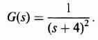
   Figure P7.5 (a) Location of rudder, elevators, and ailerons on an airplane. (b) Simplified block diagram to control the roll of the airplane.

   1. Draw the root locus of this system assuming that the compensator's transfer function G_c(s) = 1.
   2. With G_c(s) = 1, determine the gain K from the root-locus diagram in order that the system has a damping ratio of 0.95. Assume that the transient behavior of the system is controlled by a pair of dominant complex-conjugate roots.
   3. It is desired that the system have a velocity constant of 40. Determine the increase in gain and the phase-lag network required to obtain a velocity constant of 40 and maintain a 0.95 damping ratio.
   4. Redraw the root locus for the compensated system. What is the new value of K for the compensated system? How does this affect the compensation G_c(s) determined in part (c)?
6. 7.6. We wish to design a combined compensator of a regulator that includes a controller and an estimator for a chemical process control system. Assume that the transfer function of the chemical process to be controlled is given by

   

   Assume that the design specification of the controller is that it be critically damped with an ω_n = 2 rad/sec, and that the estimator is also critically damped but with an ω_n = 10 rad/sec,

   1. Find the controller's gain coefficients' matrix.
   2. Find the estimator's coefficients' vector.
   3. Design the compensator for the combined controller and estimator.
   4. Draw the root locus of the compensated system, and find the location of all the roots of the compensated system.
   5. Draw the Bode diagram for the compensated system,. Find its gain crossover frequency, phase margin, phase crossover frequency, and gain margin.
   6. How does the gain crossover frequency of part (e) compare with the controller's and estimator's closed-loop roots specified? Is this reasonable?
   7. Determine the transient response of the compensated system to a unit step input.
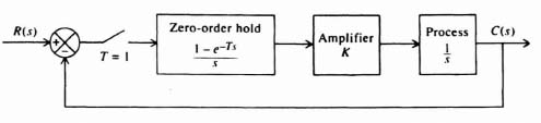
7. 7.7. A student is experimenting with a simple sampled-data control system in the laboratory for the first time. The block diagram of the system he is experimenting with is shown in Figure P7.7. To determine the effect of the amplifier gain K on system stability, the student increases the gain K from zero to three. What kind of response to a unit step input will the student find for the following values of gain K:
   1. K = 0.5;
   2. K = 1;
   3. K = 2;
   4. K = 3.

   

   Figure P7.7

8. 7.8. The design of the positioning system of a tracking radar is a very interesting control-system problem. Figure P7.8a illustrates a tracking radar which has wind torque disturbances acting on it, and the equivalent block diagram for one axis of the tracking radar's positioning loop is illustrated in Figure P7.8b. The block diagram illustrated represents a two-degrees-of-freedom robust control system which has the dual capability of minimizing the effects of the wind torque disturbance D(s) while also being robust (insensitive) to variations in the gain K. The transfer function for the forward-loop transfer function for the tracking radar G₀(s) is given by

   

   

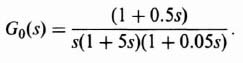
   Figure P7.8 A tracking radar conceptually illustrating disturbance torques due to wind forces (a) and the equivalent block diagram of the tracking radar's positioning loop (b).

   1. Determine the transient response of this control system to a unit step input at R(s) assuming that G_c1(s) = G_c2(s) = 1 and K has a nominal value of 130, but can also be as low as 20 or as high as 200.
   2. Draw the root locus for the conditions in part (a). Determine the location of the closed roots for K = 20, 130, and 200, and determine the damping ratio for the dominant complex-conjugate roots for these three cases.
   3. Design G_c2(s) so that it contains the zeros which cancel the complex-conjugate roots for the case of nominal gain of 130.
   4. Draw the root locus for the conditions of part (c). Determine the location of the closed-loop roots for K = 20, 130, and 200, and determine the damping ratio for the dominant complex-conjugate roots for these three cases.
   5. Design the series controller G_c1(s) and plot the resulting transient response of this control system containing G_c1(s) and G_c2(s) which was designed in part (c).
   6. How do the transient responses of part (e) compare with the transient responses of part (a)? Discuss the robustness of your resulting design to variations in the gain K.

REFERENCES

1. S. M. Shinners, Techniques of System Engineering, Chapter 8. McGraw-Hili, New York, 1967.

2. S. M. Shinners, A Guide to Systems Engineering and Management. Lexington Books, Lexington, MA, 1976.

3. P. M. Lowitt and S. M. Shinners, “Integrated optimal synthesis for a tracking radar.” In Proceedings of the 7th National Military Electronics Convention, Washington, DC. 74–78 September, 1963.

4. P. M. Lowitt and S. M. Shinners, “‘Type-N integral space tracking configurations.” IEEE Trans. Mil. Electron. 416–424 (1965).

5. C. L. Phillips and H. T. Nagle, Jr., Digital Control System Analysis and Design. Prentice-Hall, Englewood Cliffs, NJ, 1984.

6. R. Y. Chiang and M. G. Safonou, “Modern CACSD Using the Robust Control Toolbox.” Proc. Canf. on Aerospace and Computational Control, Oxnard, CA, August 28–30, 1989.

7. P. Dorato, Robust Control. IEEE Press, New York, 1987.

8. P. Dorato, “Case Studies in Robust Control Design.” IEEE Proc. Decision and Control Conf., December, 1990.

9. B. C. Kuo, Automatic Control Systems. Prentice Hall, Englewood Cliffs, NJ, 1995.

10. P. A. Ioannou and J. Sun, Robust Adaptive Control. Prentice Hall Professional Technical Reference, Des Moines, IA, 1995.