Chapter 2
The Physics of Light Transport
The goal of rendering algorithms is to create images that accurately represent the appearance of objects in scenes. For every pixel in an image, these algorithms must find the objects that are visible at that pixel and then display their “appearance” to the user. What does the term “appearance” mean? What quantity of light energy must be measured to capture “appearance”? How is this energy computed? These are the questions that this chapter will address.
In this chapter, we present key concepts and definitions required to formulate the problem that global illumination algorithms must solve. In Section 2.1, we present a brief history of optics to motivate the basic assumptions that rendering algorithms make about the behavior of light (Section 2.2). In Section 2.3, we define radiometric terms and their relations to each other. Section 2.4 describes the sources of lights in scenes; in Section 2.5, we present the bidirectional distribution function, which captures the interaction of light with surfaces. Using these definitions, we present the rendering equation in Section 2.6, a mathematical formulation of the equilibrium distribution of light energy in a scene. We also formulate the notion of importance in Section 2.7. Finally, in Section 2.8, we present the measurement equation, which is the equation that global illumination algorithms must solve to compute images. In the rest of this book, we will discuss how global illumination algorithms solve the measurement equation.
2.1 Brief History
The history of the science of optics spans about three thousand years of human history. We briefly summarize relevant events based mostly on the history included by Hecht and Zajac in their book Optics [68]. The Greek philosophers (around 350 B.C.), including Pythagoras, Democritus, Empedocles, Plato, and Aristotle among others, evolved theories of the nature of light. In fact, Aristotle’s theories were quite similar to the ether theory of the nineteenth century. However, the Greeks incorrectly believed that vision involved emanations from the eye to the object perceived. By 300 B.C. the rectilinear propagation of light was known, and Euclid described the law of reflection. Cleomedes (50 A.D.) and Ptolemy (130 A.D.) did early work on studying the phenomenon of refraction.
The field of optics stayed mostly dormant during the Dark Ages with the exception of the contribution of Ibn-al-Haitham (also known as Al-hazen); Al-hazen refined the law of reflection specifying that the angles of incidence and reflection lie in the same plane, normal to the interface. In fact, except for the contributions of Robert Grosseteste (1175–1253) and Roger Bacon (1215–1294) the field of optics did not see major activity until the seventeenth century.
Optics became an exciting area of research again with the invention of telescopes and microscopes early in the seventeenth century. In 1611, Johannes Kepler discovered total internal reflection and described the small angle approximation to the law of refraction. In 1621, Willebrord Snell made a major discovery: the law of refraction; the formulation of this law in terms of sines was later published by Ren´e Descartes. In 1657, Pierre de Fermat rederived the law of refraction from his own principle of least time, which states that a ray of light follows the path that takes it to its destination in the shortest time.
Diffraction, the phenomenon where light “bends” around obstructing objects, was observed by Grimaldi (1618–1683) and Hooke (1635–1703). Hooke first proposed the wave theory of light to explain this behavior. Christian Huygens (1629–1695) considerably extended on the wave theory of light. He was able to derive the laws of reflection and refraction using this theory; he also discovered the phenomenon of polarization during his experiments.
Contemporaneously, Isaac Newton (1642–1727) observed dispersion, where white light splits into its component colors when it passes through a prism. He concluded that sunlight is composed of light of different colors, which are refracted by glass to different extents. Newton, over the course of his research, increasingly embraced the emission (corpuscular) theory of light over the wave theory.
Thus, in the beginning of the nineteenth century, there were two conflicting theories of the behavior of light: the particle (emission/corpuscular) theory and the wave theory. In 1801, Thomas Young described his principle of interference based on his famous double-slit experiment, thus providing experimental support for the wave theory of light. However, due to the weight of Newton’s influence, his theory was not well-received. Independently, in 1816, Augustin Jean Fresnel presented a rigorous treatment of diffraction and interference phenomena showing that these phenomena can be explained in terms of the wave theory of light. In 1821, Fresnel presented the laws that enable the intensity and polarization of reflected and refracted light to be calculated.
Independently in the field of electricity and magnetism, Maxwell (1831-1879) summarized and extended the empirical knowledge on these subjects into a single set of mathematical equations. Maxwell concluded that light is a form of electromagnetic wave. However, in 1887, Hertz accidentally discovered the photoelectric effect: the process whereby electrons are liberated from materials under the action of radiant energy. This effect could not be explained by the wave model of light. Other properties of light also remained inexplicable in the wave model: black body radiation (the spectrum of light emitted by a heated body), the wavelength dependency of the absorption of light by various materials, fluorescence1, and phosphorescence2, among others. Thus, despite all the supporting evidence for the wave nature of light, the particle behavior of light had to be explained.
In 1900, Max Karl Planck introduced a universal constant called Planck’s constant to explain the spectrum of radiation emitted from a hot black body: black body radiation. His work inspired Albert Einstein, who, in 1905, explained the photoelectric effect based on the notion that light consists of a stream of quantized energy packets. Each quantum was later called a photon. Each photon has a frequency ν associated with it. The energy associated with a photon is E = ħν, where ħ is Planck’s constant.
The seemingly conflicting behavior of light as a stream of particles and waves was only reconciled by the establishment of the field of quantum mechanics. By considering submicroscopic phenomena, researchers such as Bohr, Born, Heisenberg, Schrödinger, Pauli, de Broglie, Dirac, and others were able to explain the dual nature of light. Quantum field theory and quantum electrodynamics further explained high-energy phenomena; Richard Feynman’s book on quantum electrodynamics (QED) [49] gives an intuitive description of the field.
2.2 Models of Light
The models of light used in simulations try to capture the different behaviors of light that arise from its dual nature: certain phenomena, for example, diffraction and interference, can be explained by assuming that light is a wave; other behavior, such as the photoelectric effect, can be better explained by assuming that light consists of a stream of particles.
2.2.1 Quantum Optics
Quantum optics is the fundamental model of light that explains its dual wave-particle nature. The quantum optics model can explain the behavior of light at the submicroscopic level, for example, at the level of electrons. However, this model is generally considered to be too detailed for the purposes of image generation for typical computer graphics scenes and is not commonly used.
2.2.2 Wave Model
The wave model, a simplification of the quantum model, is described by Maxwell’s equations. This model captures effects, such as diffraction, interference, and polarization, that arise when light interacts with objects of size comparable to the wavelength of light. These effects can be observed in everyday scenes, for example, in the bright colors seen in oil slicks or birds’ feathers. However, for the purposes of image generation in computer graphics, the wave nature of light is also typically ignored.
2.2.3 Geometric Optics
The geometric optics model is the simplest and most commonly used model of light in computer graphics. In this model, the wavelength of light is assumed to be much smaller than the scale of the objects that the light interacts with. The geometric optics model assumes that light is emitted, reflected, and transmitted. In this model, several assumptions are made about the behavior of light:
- Light travels in straight lines, i.e., effects such as diffraction where light “bends around” objects are not considered.
- Light travels instantaneously through a medium; this assumption essentially requires light to unrealistically travel at infinite speed. However, it is a practical assumption because it requires global illumination algorithms to compute the steady-state distribution of light energy in scenes.
- Light is not influenced by external factors, such as gravity or magnetic fields.
In most of this book, we ignore effects that arise due to the transmission of light through participating media (for example, fog). We also do not consider media with varying indices of refraction. For example, mirage-like effects that arise due to varying indices of refraction caused by temperature differentials in the air are not considered. How to deal with these phenomena is discussed in Section 8.1.
2.3 Radiometry
The goal of a global illumination algorithm is to compute the steady-state distribution of light energy in a scene. To compute this distribution, we need an understanding of the physical quantities that represent light energy. Radiometry is the area of study involved in the physical measurement of light. This section gives a brief overview of the radiometric units used in global illumination algorithms.
It is useful to consider the relation between radiometry and photometry. Photometry is the area of study that deals with the quantification of the perception of light energy. The human visual system is sensitive to light in the frequency range of 380 nanometers to 780 nanometers. The sensitivity of the human eye across this visible spectrum has been standardized; photometric terms take this standardized response into account. Since photometric quantities can be derived from the corresponding radiometric terms, global illumination algorithms operate on radiometric terms. However, Section 8.2 will talk about how the radiometric quantities computed by global illumination algorithms are displayed to an observer.
2.3.1 Radiometric Quantities
Radiant Power or Flux
The fundamental radiometric quantity is radiant power, also called flux. Radiant power, often denoted as Φ, is expressed in watts (W) (joules/sec). This quantity expresses how much total energy flows from/to/through a surface per unit time. For example, we can say that a light source emits 50 watts of radiant power, or that 20 watts of radiant power is incident on a table. Note that flux does not specify the size of the light source or the receiver (table), nor does it include a specification of the distance between the light source and the receiver.
Irradiance
Irradiance (E) is the incident radiant power on a surface, per unit surface area. It is expressed in watts/m2:
E=dΦdA. (2.1)
For example, if 50 watts of radiant power is incident on a surface that has an area of 1.25 m2, the irradiance at each surface point is 40 watts/m2 (assuming the incident power is uniformly distributed over the surface).
Radiant Exitance or Radiosity
Radiant exitance (M), also called radiosity (B), is the exitant radiant power per unit surface area and is also expressed in watts/m2:
M=B=dΦdA. (2.2)
For example, consider a light source, of area 0.1 m2, that emits 100 watts. Assuming that the power is emitted uniformly over the area of the light source, the radiant exitance of the light is 1000 W/m2 at each point of its surface.
Radiance
Radiance is flux per unit projected area per unit solid angle (watts/(steradian · m2)). Intuitively, radiance expresses how much power arrives at (or leaves from) a certain point on a surface, per unit solid angle, and per unit projected area. Appendix B gives a review of solid angles and hemispherical geometry.
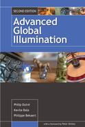
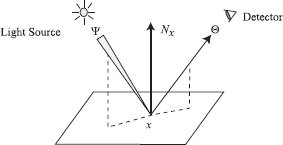
Radiance is a five-dimensional quantity that varies with position x and direction vector Θ, and is expressed as L(x, Θ) (see Figure 2.1):
L=d2ΦdωdA⊥=d2ΦdωdAcos θ. (2.3)
Definition of radiance L(x, Θ): flux per unit projected area dA⊥ per unit solid angle dω.
Radiance is probably the most important quantity in global illumination algorithms because it is the quantity that captures the “appearance” of objects in the scene. Section 2.3.3 explains the properties of radiance that are relevant to image generation.
Intuition for cosine term. The projected area A⊥ is the area of the surface projected perpendicular to the direction we are interested in. This stems from the fact that power arriving at a grazing angle is “smeared out” over a larger surface. Since we explicitly want to express power per (unit) projected area and per (unit) direction, we have to take the larger area into account, and that is where the cosine term comes from. Another intuition for this term is obtained by drawing insights from transport theory.
Transport Theory
This section uses concepts from transport theory to intuitively explain the relations between different radiometric terms (see Chapter 2, [29]). Transport theory deals with the transport or flow of physical quantities such as energy, charge, and mass. In this section, we use transport theory to formulate radiometric quantities in terms of the flow of “light particles” or “photons.”
Let us assume we are given the density of light particles, p(x), which defines the number of particles per unit volume at some position x. The number of particles in a small volume dV is p(x)dV. Let us consider the flow of these light particles in some time dt across some differential surface area dA. Assume that the velocity of the light particles is →c, where |→c| is the speed of light and the direction of →c is the direction along which the particles are flowing. Initially, we assume that the differential surface area dA is perpendicular to the flow of particles. Given these assumptions, in time dt, the particles that flow across the area dA are all the particles included in a volume cdtdA. The number of particles flowing across the surface is p(x)cdtdA.

We now relax the assumption that the particle flow is perpendicular to the surface area dA (as shown in Figure 2.2). If the angle between the flow of the particles and dA is θ, the perpendicular area across which the particles flow is dA cos θ. Now, the number of particles flowing across the surface is p(x)cdtdA cos θ.
The derivation above assumed a fixed direction of flow. Including all possible directions (and all possible wavelengths) along which the particles can flow gives the following number of particles N that flow across an area dA,
N=p(x,ω,λ)cdtdA cos θdωdλ,
where dω is a differential direction (or solid angle) along which particles flow and the density function p varies with both position and direction.
Flux is defined as the energy of the particles per unit time. In this treatment, flux is computed by dividing the number of particles by dt and computing the limit as dt goes to zero:
Φ∝p(x,ω,λ)dAcos θdωdλ,ΦdAcos θdω∝p(x,ω,λ)dλ.
Let us assume these particles are photons. Each photon has energy E = ħν. The wavelength of light λ is related to its frequency by the following relation: λ = c/ν, where c is the speed of light in vacuum. Therefore, E=ℏcλ. Nicodemus [131] defined radiance as the radiant energy per unit volume, as follows:
L(x,ω)=∫p(x,ω,λ)ℏcλdλ.
Relating this equation with the definition of Φ above, we get a more intuitive notion of how flux relates to radiance, and why the cosine term arises in the definition of radiance.
2.3.2 Relationships between Radiometric Quantities
Given the definitions of the radiometric quantities above, the following relationships between these different terms can be derived:
Φ=∫A∫ΩL(x→Θ) cosθ dωΘ dAx,(2.4)E(x)=∫ΩL(x←Θ) cosθ dωΘ,(2.5)B(x)=∫ΩL(x→) cosθ dωΘ,(2.6)
where A is the total surface area and Ω is the total solid angle at each point on the surface.
We use the following notation in this book: L(x → Θ) represents radiance leaving point x in direction Θ. L(x ← Θ) represents radiance arriving at point x from direction Θ.
Wavelength Dependency
The radiometric measures and quantities described above are not only dependent on position and direction but are also dependent on the wavelength of light energy. When wavelength is explicitly specified, for example, for radiance, the corresponding radiometric quantity is called spectral radiance. The units of spectral radiance are the units of radiance divided by meters (the unit of wavelength). Radiance is computed by integrating spectral radiance over the wavelength domain covering visible light. For example,
L(x→Θ)=∫spectrumL(x→Θ,λ)dλ.
The wavelength dependency of radiometric terms is often implicitly assumed to be part of the global illumination equations and is not mentioned explicitly.
2.3.3 Properties of Radiance
Radiance is a fundamental radiometric quantity for the purposes of image generation. As seen in Equations 2.4–2.6, other radiometric terms, such as flux, irradiance, and radiosity can be derived from radiance. The following properties of radiance explain why radiance is important for image generation.
Property 1: Radiance is invariant along straight paths.
Mathematically, the property of the invariance of radiance is expressed as
L(x→y)=L(y←x),
which states that the radiance leaving point x directed towards point y is equal to the radiance arriving at point y from the point x. This property assumes that light is traveling through a vacuum, i.e., there is no participating medium.
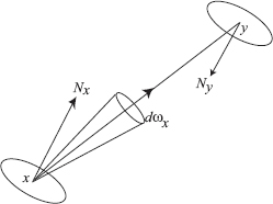
This important property follows from the conservation of light energy in a small pencil of rays between two differential surfaces at x and y, respectively. Figure 2.3 shows the geometry of the surfaces. From the definition of radiance, the total (differential) power leaving a differential surface area dAx, and arriving at a differential surface area dAy, can be written as

L(x→y)=d2Φ(cosθxdAx)dωx←dAy;(2.7)d2Φ=L(x→y) cosθxdωx←dAy dAx,(2.8)
where we use the notation that dωx ← dAy is the solid angle subtended by dAy as seen from x.
The power that arrives at area dAy from area dAx can be expressed in a similar way:
L(y←x)=d2Φ(cosθydAy)dωy←dAx;(2.9)d2Φ=L(y←x) cosθydωy←dAx dAy.(2.10)
The differential solid angles are:
dωx←dAy=cosθydAyr2xy;dωy←dAx=cosθxdAxr2xy.
We assume that there are no external light sources adding to the power arriving at dAy. We also assume that the two differential surfaces are in a vacuum; therefore, there is no energy loss due to the presence of participating media. Then, by the law of conservation of energy, all energy leaving dAx in the direction of the surface dAy must arrive at dAy,
L(x→y) cosθxdωx←dAy dAx=L(y←x) cosθydωy←dAx dAy;L(x→y) cosθxcosθydAyr2xy dAx=L(y←x) cosθycosθxdAxr2xy dAy,
and thus,
L(x→y) = L(y←x). (2.11)
Therefore, radiance is invariant along straight paths of travel and does not attenuate with distance. This property of radiance is only valid in the absence of participating media, which can absorb and scatter energy between the two surfaces.
From the above observation, it follows that once incident or exitant radiance at all surface points is known, the radiance distribution for all points in a three-dimensional scene is also known. Almost all algorithms used in global illumination limit themselves to computing the radiance values at surface points (still assuming the absence of any participating medium). Radiance at surface points is referred to as surface radiance by some authors, whereas radiance for general points in three-dimensional space is sometimes called field radiance.
Property 2: Sensors, such as cameras and the human eye, are sensitive to radiance.
The response of sensors (for example, cameras or the human eye) is proportional to the radiance incident upon them, where the constant of proportionality depends on the geometry of the sensor.
These two properties explain why the perceived color or brightness of an object does not change with distance. Given these properties, it is clear that radiance is the quantity that global illumination algorithms must compute and display to the observer.
2.3.4 Examples
This section gives a few practical examples of the relationship between the different radiometric quantities that we have seen.
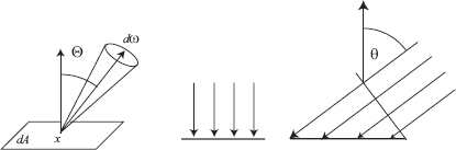
Example (Diffuse Emitter)
Let us consider the example of a diffuse emitter. By definition, a diffuse emitter emits equal radiance in all directions from all its surface points (as shown in Figure 2.4). Therefore,
L(x→Θ)=L.
The power for the diffuse emitter can be derived as
Φ=∫A∫ΩL(x→Θ)cos θdωΘdAx=∫A∫ΩLcos θdωΘdAx=L(∫AdAx)(∫Ωcos θdωΘ)=πLA,
where A is the area of the diffuse emitter, and integration at each point on A is over the hemisphere, i.e., Ω is the hemisphere at each point (see Appendix B).
The radiance for a diffuse emitter equals the power divided by the area, divided by π. Using the above equations, it is straightforward to write down the following relationship between the power, radiance, and radiosity of a diffuse surface:
Φ=LAπ=BA. (2.12)
Example (Nondiffuse Emitter)
Consider a square area light source with a surface area measuring 10 × 10 cm2. Each point on the light source emits radiance according to the following distribution over its hemisphere:
L(x→Θ)=6000cos θ(W/sr.m2).
Remember that the radiance function is defined for all directions on the hemisphere and all points on a surface. This specific distribution is the same for all points on the light source. However, for each surface point, there is a fall-off as the direction is farther away from the normal at that surface point.
The radiosity for each point can be computed as follows:
B=∫ΩL(x→Θ)cos θdωΘ =∫Ω6000 cos 2θdωΘ =6000∫2π0∫π/20 cos 2θsin θdθdϕ =6000·2π·[−cos 3θ3]π/20 =4000π W/m2 =12566 W/m2.
The power for the entire light source can then be computed as follows:
Φ=∫A∫ΩL(x→Θ)cos θdωΘdAx =∫A(∫ΩLcos θdωΘ)dAx =∫AB(x)dAx =4000π W/m2 ·0.1 m·0.1 m =125.66 W.
Example (Sun, Earth, Mars)
Now let us consider the example of an emitter that is very important to us: the Sun. One might ask the question, if the radiance of the Sun is the same irrespective of the distance from the Sun, why is the Earth warmer than Mars?
Consider the radiance output from the Sun arriving at the Earth and Mars (see Figure 2.5). For simplicity, let us assume that the Sun is a uniform diffuse emitter. As before, we assume that the medium between the Earth, Sun, and Mars is a vacuum. From Equation 2.12,

Φ=πLA.
Given that the total power emitted by the Sun is 3.91 × 1026 watts, and the surface area of the Sun is 6.07 × 10¹⁸ m2, the Sun’s radiance equals
L(Sun)=ΦAπ=3.91×1026π6.07×1018=2.05×10⁷ W/sr·m2.
Now consider a 1 × 1 m2 patch on the surface of the Earth; the power arriving at that patch is
P(Earth←Sun)=∫A∫ΩLcos θdωdA.
Let us also assume that the Sun is at its zenith (i.e., cosθ = 1), and that the solid angle subtended by the Sun is small enough that the radiance can be assumed to be constant over the patch:
P(Earth←Sun)=ApatchLω.
The solid angle ω subtended by the Sun as seen from the Earth is
ωEarth←sun=A⊥sundiskdistance2=6.7×10⁻⁵sr.
Note that the area of the Sun considered for the computation of the radiance of the Sun is its surface area, whereas the area of the Sun in the computation of the solid angle is the area of a circular section (disc) of the Sun; this area is 1/4th the surface area of the Sun:
P(Earth←Sun)=(1×1 m2)(2.05×10⁷ W/(sr·m2))(6.7×10−5sr) =1373.5 W.
Similarly, consider a 1 × 1 m2 patch on the surface of Mars, the power arriving at that patch can be computed in the same way. The solid angle subtended by the Sun as seen from Mars is
ωMars←sun=A⊥sundiskdistance2=2.92×10⁻⁵sr.
The total power incident on the patch on Mars is given by
P(Mars←Sun)=(1×1 m2)(2.05×10⁷ W/( sr·m2))(2.92×10⁻⁵sr) =598.6 W.
Thus, even though the radiance of the Sun is invariant along rays and is the same as seen from the Earth and Mars, the solid angle measure ensures that the power arriving at the planets drops off as the square of the distance (the familiar inverse square law). Therefore, though the Sun will appear equally bright on the Earth and Mars, it will look larger on the Earth than on Mars and, therefore, warm the planet more.
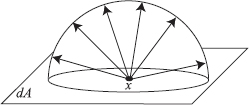
Example (Plate)
A flat plate is placed on top of Mount Everest with its normal pointing up (See Figure 2.6). It is a cloudy day, and the sky has a uniform radiance of 1000 W/(sr · m2). The irradiance at the center of the plate can be computed as follows:
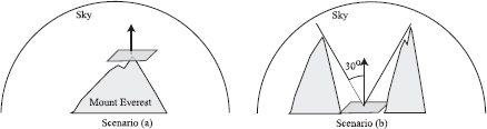
Plate with different constraints on incoming hemisphere. Scenario (a): plate at top of peak; Scenario (b): plate in valley with 60° cutoff.
E=∫L(x←Θ)cosθdω =1000∫∫cosθ sinθdθdϕ =1000∫2π0dϕ ∫π/20cosθsinθdθ =1000⋅2π⋅[−cos2θ2]π/20 =1000⋅2π⋅12 =1000⋅π W/m2⋅
Now assume the plate is taken to an adjoining valley where the surrounding mountains are radially symmetric and block off all light below 60°. The irradiance at the plate in this situation is
E=∫L(x←Θ)cosθdω =1000∫∫cosθ sinθdθdϕ =1000∫2π0dϕ ∫π/60cosθsinθdθ =1000⋅2π⋅[−cos2θ2]π/60 =1000⋅π⋅(1−34) =250⋅πW/m2⋅
2.4 Light Emission
Light is electromagnetic radiation produced by accelerating a charge. Light can be produced in different ways; for example, by thermal sources such as the sun, or by quantum effects such as fluorescence, where materials absorb energy at some wavelength and emit the energy at some other wavelength. As mentioned in previous sections, we do not consider a detailed quantum mechanical explanation of light for the purposes of computer graphics. In most rendering algorithms, light is assumed to be emitted from light sources at a particular wavelength and with a particular intensity.
The computation of accurate global illumination requires the specification of the following three distributions for each light source: spatial, directional, and spectral intensity distribution. For example, users, such as lighting design engineers, require accurate descriptions of light source distributions that match physical light bulbs available in the real world. Idealized spatial distributions of lights assume lights are point lights; more realistically, lights are modeled as area lights. The directional distributions of typical luminaires is determined by the shape of their associated light fixtures. Though the spectral distribution of light could also be simulated accurately, global illumination algorithms typically simulate RGB (or a similar triple) for efficiency reasons. All these distributions could be specified either as functions or as tables.
2.5 Interaction of Light with Surfaces
Light energy emitted into a scene interacts with the different objects in the scene by getting reflected or transmitted at surface boundaries. Some of the light energy could also be absorbed by surfaces and dissipated as heat, though this phenomenon is typically not explicitly modeled in rendering algorithms.
2.5.1 BRDF
Materials interact with light in different ways, and the appearance of materials differs given the same lighting conditions. Some materials appear as mirrors; others appear as diffuse surfaces. The reflectance properties of a surface affect the appearance of the object. In this book, we assume that light incident at a surface exits at the same wavelength and same time. Therefore, we are ignoring effects such as fluorescence and phosphorescence.
In the most general case, light can enter some surface at a point p and incident direction Ψ and can leave the surface at some other point q and exitant direction Θ. The function defining this relation between the incident and reflected radiance is called the bidirectional surface scattering reflectance distribution function (BSSRDF) [131]. We make the additional assumption that the light incident at some point exits at the same point; thus, we do not discuss subsurface scattering, which results in the light exiting at a different point on the surface of the object.
Given these assumptions, the reflectance properties of a surface are described by a reflectance function called the bidirectional reflectance distribution function (BRDF). The BRDF at a point x is defined as the ratio of the differential radiance reflected in an exitant direction (Θ), and the differential irradiance incident through a differential solid angle (dωΨ,). The BRDF is denoted as fr (x, Ψ → Θ):
fr(x, Ψ→Θ)=dL(x→Θ)dE(x←Ψ)(2.13)=dL(x→Θ)L(x←Ψ) cos(Nx, Ψ) dωΨ,(2.14)
where cos(Nx, Ψ) is the cosine of the angle formed by the normal vector at the point x, Nx, and the incident direction vector Ψ.
Strictly speaking, the BRDF is defined over the entire sphere of directions (4π steradians) around a surface point. This is important for transparent surfaces, since these surfaces can “reflect” light over the entire sphere. In most texts, the term BSDF (bidirectional scattering distribution function) is used to denote the reflection and transparent parts together.
2.5.2 Properties of the BRDF
There are several important properties of a BRDF:
- Range. The BRDF can take any positive value and can vary with wavelength.
Dimension. The BRDF is a four-dimensional function defined at each point on a surface; two dimensions correspond to the incoming direction, and two dimensions correspond to the outgoing direction.
Generally, the BRDF is anisotropic. That is, if the surface is rotated about the surface normal, the value of fr will change. However, there are many isotropic materials for which the value of fr does not depend on the specific orientation of the underlying surface.
Reciprocity. The value of the BRDF remains unchanged if the incident and exitant directions are interchanged. This property is also called Helmholtz reciprocity; intuitively, it means that reversing the direction of light does not change the amount of light that gets reflected:
fr(x,Ψ→Θ)=fr(x,Θ→Ψ).
Because of the reciprocity property, the following notation is used for the BRDF to indicate that both directions can be freely interchanged:
fr(x,Θ↔Ψ).
Relation between incident and reflected radiance. The value of the BRDF for a specific incident direction is not dependent on the possible presence of irradiance along other incident angles. Therefore, the BRDF behaves as a linear function with respect to all incident directions. The total reflected radiance due to some irradiance distribution over the hemisphere around an opaque, non-emissive surface point can be expressed as:
dL(x→Θ)=fr(x, Ψ→Θ)dE(x←Ψ);(2.15)L(x→Θ)=∫Ωxfr(x, Ψ→Θ)dE(x←Ψ);(2.16)L(x→Θ)=∫Ωxfr(x, Ψ→Θ)L(x←Ψ) cos(Nx, Ψ)dωΨ.(2.17)
Energy conservation. The law of conservation of energy requires that the total amount of power reflected over all directions must be less than or equal to the total amount of power incident on the surface (excess power is transformed into heat or other forms of energy). For any distribution of incident radiance L(x ← Ψ) over the hemisphere, the total incident power per unit surface area is the total irradiance over the hemisphere:
E=∫ΩxL(x←Ψ)cos(Nx,Ψ)dωΨ. (2.18)
The total reflected power M is a double integral over the hemisphere. Suppose we have a distribution of exitant radiance L(x → Θ) at a surface. The total power per unit surface area leaving the surface, M, is
M=∫ΩxL(x→Θ)cos(Nx,Θ)dωΘ. (2.19)
From the definition of the BRDF, we know
dL(x→Θ)=fr(x,Ψ→Θ)L(x←Ψ)cos(Nx,Ψ)dωΨ.
Integrating this equation to find the value for L(x → Θ) and combining it with the expression for M gives us
M=∫Ωx∫Ωxfr(x,Ψ→Θ)L(x←Ψ)cos(Nx,Θ)cos(Nx,Ψ)dωΨdωΘ. (2.20)
The BRDF satisfies the constraint of energy conservation for reflectance at a surface point if, for all possible incident radiance distributions L(x ← Ψ), the following inequality holds: M ≤ E, or
∫Ωx∫Ωxfr(x,Ψ→Θ)L(x←Ψ)cos(Nx,Θ)cos(Nx,Ψ)dωΨdωΘ∫ΩxL(x←Ψ)cos(Nx,Ψ)dωΨ≤1. (2.21)
This inequality must be true for any incident radiance function. Suppose we take an appropriate δ-function for the incident radiance distribution, such that the integrals become simple expressions:
L(x←Ψ)=Linδ(Ψ−Θ),
then, the above equation can be simplified to
∀Ψ:∫Ωxfr(x,Ψ→Θ)cos(Nx,Θ)dωΘ≤1. (2.22)
The above equation is a necessary condition for energy conservation, since it expresses the inequality for a specific incident radiance distribution. It is also a sufficient condition because incident radiance from two different directions do not influence the value of the BRDF; therefore, conservation of energy is valid for any combination of incident radiance values. If the value of the BRDF is dependent on the intensity of the incoming light, the more elaborate inequality from Equation 2.21 holds.
Global illumination algorithms often use empirical models to characterize the BRDF. Great care must be taken to make certain that these empirical models are a good and acceptable BRDF. More specifically, energy conservation and Helmholtz reciprocity must be satisfied to make an empirical model physically plausible.
Satisfying Helmholtz reciprocity is a particularly important constraint for bidirectional global illumination algorithms; these algorithms compute the distribution of light energy by considering paths starting from the light sources and paths starting from the observer at the same time. Such algorithms explicitly assume that light paths can be reversed; therefore, the model for the BRDF should satisfy Helmholtz’s reciprocity.
2.5.3 BRDF Examples
Depending on the nature of the BRDF, the material will appear as a diffuse surface, a mirror, or a glossy surface (see Figure 2.8). The most commonly encountered types of BRDFs are listed below.
Diffuse Surfaces
Some materials reflect light uniformly over the entire reflecting hemisphere. That is, given an irradiance distribution, the reflected radiance is independent of the exitant direction. Such materials are called diffuse reflectors, and the value of their BRDF is constant for all values of Θ and Ψ. To an observer, a diffuse surface point looks the same from all possible directions. For an ideal diffuse surface,
fr(x,Ψ↔Θ)=ρdπ. (2.23)
The reflectance ρd represents the fraction of incident energy that is reflected at a surface. For physically-based materials, ρd varies from 0 to 1. The reflectance of diffuse surfaces is used in radiosity calculations as will be seen in Chapter 6.
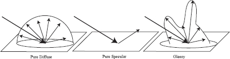
Specular Surfaces
Perfect specular surfaces only reflect or refract light in one specific direction.
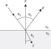
Specular reflection. The direction of reflection can be found using the law of reflection, which states that the incident and exitant light direction make equal angles to the surface’s normal, and lie in the same plane as the normal. Given that light is incident to the specular surface along direction vector Ψ, and the normal to the surface is N, the incident light is reflected along the direction R:
R=2(N⋅Ψ)N−Ψ. (2.24)
A perfect specular reflector has only one exitant direction for which the BRDF is different from 0; the implication is that the value of the BRDF along that direction is infinite. The BRDF of such a perfect specular reflector can be described with the proper use of δ-functions. Real materials can exhibit this behavior very closely, but are nevertheless not ideal reflectors as defined above.
Specular refraction. The direction of specular refraction is computed using Snell’s law. Consider the direction T along which light that is incident from a medium with refractive index η1 to a medium with refractive index η2 is refracted. Snell’s law specifies the following invariant between the angle of incidence and refraction and the refractive indices of the media:
η1 sinθ1=η2 sinθ2, (2.25)
where θ1 and θ2 are the angles between the incident and transmitted ray and the normal to the surface.
The transmitted ray T is given as:
T=−η1η2Ψ+N(η1η2cos θ1−√1−(η1η2)2(1−cos θ21)), =−η1η2Ψ+N(η1η2(N⋅Ψ)−√1−(η1η2)2(1−(N⋅Ψ)2)), (2.26)
since cosθ1 = N · Ψ, the inner product of the normal and the incoming direction.
When light travels from a dense medium to a rare medium, it could get refracted back into the dense medium. This process is called total internal reflection; it arises at a critical angle θc, also known as Brewster’s angle, which can be computed by Snell’s law:
η1sinθc=η2sinπ2;sinθc=η2η1⋅
We can derive the same condition from Equation 2.26, where total internal reflection occurs when the term under the square root, 1−(η1η2)2(1−cos θ21), is less than zero.
Figure 2.9 shows the geometry of perfect specular reflections and refractions.
Reciprocity for transparent surfaces. One has to be careful when assuming properties about the transparent side of the BSDF; some characteristics, such as reciprocity, may not be true with transparent surfaces as described below. When a pencil of light enters a dense medium from a less dense (rare) medium, it gets compressed. This behavior is a direct consequence of Snell’s law of refraction (rays “bend” towards the normal direction). Therefore, the light energy per unit area perpendicular to the pencil direction becomes higher; i.e., the radiance is higher. The reverse process takes place when a pencil of light leaves a dense medium to be refracted into a less dense medium. The change in ray density is the square ratio of the refractive indices of the media [203, 204]: (η2/η1)2. When computing radiance in scenes with transparent surfaces, this weighting factor should be considered.
Fresnel equations. The above equations specify the angles of reflection and refraction for light that arrives at a perfectly smooth surface. Fresnel derived a set of equations called the Fresnel equations that specify the amount of light energy that is reflected and refracted from a perfectly smooth surface.
When light hits a perfectly smooth surface, the light energy that is reflected depends on the wavelength of light, the geometry at the surface, and the incident direction of the light. Fresnel equations specify the fraction of light energy that is reflected. These equations (given below) take the polarization of light into consideration. The two components of the polarized light, rp and rs, referring to the parallel and perpendicular (senkrecht in German) components, are given as
rp=η2 cosθ1–η1 cosθ2η2 cosθ1+η1 cosθ2; (2.27)rs=η1 cosθ1–η2 cosθ2η1 cosθ1+η2 cosθ2, (2.28)
where η1 and η2 are the refractive indices of the two surfaces at the interface.
For unpolarized light, F=|rp|2+|rs|22. Note that these equations apply for both metals and nonmetals; for metals, the index of refraction of the metal is expressed as a complex variable: n + ik, while for nonmetals, the refractive index is a real number and k = 0.
The Fresnel equations assume that light is either reflected or refracted at a purely specular surface. Since there is no absorption of light energy the reflection and refraction coefficients sum to 1.
Glossy Surfaces
Most surfaces are neither ideally diffuse nor ideally specular but exhibit a combination of both reflectance behaviors; these surfaces are called glossy surfaces. Their BRDF is often difficult to model with analytical formulae.
2.5.4 Shading Models
Real materials can have fairly complex BRDFs. Various models have been suggested in computer graphics to capture the complexity of BRDFs. Note that in the following description, Ψ is the direction of the light (the input direction) and Θ is the direction of the viewer (the outgoing direction). Lambert’s model. The simplest model is Lambert’s model for idealized diffuse materials. In this model, the BRDF is a constant as described earlier:
fr(x,Ψ↔Θ)=kd=ρdπ,
where ρd is the diffuse reflectance (see Section 2.5.3).
Phong model. Historically, the Phong shading model has been extremely popular. The BRDF for the Phong model is:
fr(x,Ψ↔Θ)=ks=(R⋅Θ)nN⋅Ψ+kd,

where the reflected vector R can be computed from Equation 2.24.
Blinn-Phong model. The Blinn-Phong model uses the half-vector H, the halfway vector between Ψ and Θ, as follows:
fr(x,Ψ↔Θ)=ks(N⋅H)nN⋅Ψ+kd.
Modified Blinn-Phong model. While the simplicity of the Phong model is appealing, it has some serious limitations: it is not energy conserving, it does not satisfy Helmholtz’s reciprocity, and it does not capture the behavior of most real materials. The modified Blinn-Phong model addresses some of these problems:
fr(x,Ψ↔Θ)=ks(N⋅H)n+kd.
Physically Based Shading Models
The modified Blinn-Phong model is still not able to capture realistic BRDFs. Physically based models, such as Cook-Torrance [33] and He [67], among others, attempt to model physical reality. We provide a brief description of the Cook-Torrance model below. For details, refer to the original paper [33]. The He model [67] is, to date, the most comprehensive and expensive shading model available; however, it is beyond the scope of this book to present this model.
Cook-Torrance model. The Cook-Torrance model includes a microfacet model that assumes that a surface is made of a random collection of small smooth planar facets. The assumption in this model is that an incoming ray randomly hits one of these smooth facets. Given a specification of the distribution of microfacets for a material, this model captures the shadowing effects of these microfacets. In addition to the facet distribution, the Cook-Torrance model also includes the Fresnel reflection and refraction terms:
fr(x,Ψ↔Θ)=F(β)πD(θh)G(N⋅Ψ)(N⋅Θ)+kd,
where the three terms in the nondiffuse component of the BRDF are the Fresnel reflectance F, the microfacet distribution D, and a geometric shadowing term G. We now present each of these terms.
The Fresnel terms, as given in Equation 2.27 and Equation 2.28, are used in the Cook-Torrance model. This model assumes that the light is unpolarized; therefore, F=|rp|2+|rs|22. The Fresnel reflectance term is computed with respect to the angle β, which is the angle between the incident direction and the half-vector: cos β = Ψ · H = Θ · H. By the definition of the half-vector, this angle is the same as the angle between the outgoing direction and the half-vector.
The distribution function D specifies the distribution of the microfacets for the material. Various functions can be used to specify this distribution. One of the most common distributions is the distribution by Beckmann:
D(θh)=1m2cos 4θhe−(tan θhm)2,
where θh is the angle between the normal and the half-vector and cos θh = N · H. Also, m is the root-mean-square slope of the microfacets, and it captures surface roughness.
The geometry term G captures masking and self-shadowing by the microfacets:
G=min {1, 2(N⋅H)(N⋅Θ)Θ⋅H,2(N⋅H)(N⋅Ψ)Θ⋅H}.
Empirical Models
Models such as Ward [221] and Lafortune [105] are based on empirical data. These models aim at ease of use and an intuitive parameterization of the BRDF. For isotropic surfaces, the Ward model has the following BRDF:
fr(x,Ψ↔Θ)=ρdπ+ρse−tan 2θhα24πα2√(N⋅Ψ)(N⋅Θ).
where θh is the angle between the half-vector and the normal.
The Ward model includes three parameters to describe the BRDF: ρd, the diffuse reflectance; ρs, the specular reflectance; and α, a measure of the surface roughness. This model is energy conserving and relatively intuitive to use because of the small set of parameters; with the appropriate parameter settings, it can be used to represent a wide range of materials. Lafortune et al. [105] introduced an empirically based model to represent measurements of real materials. This model fits modified Phong lobes to measured BRDF data. The strength of this technique is that it exploits the simplicity of the Phong model while capturing realistic BRDFs from measured data. More detailed descriptions of several models can be found in Glassner’s books [54].
2.6 Rendering Equation
Now we are ready to mathematically formulate the equilibrium distribution of light energy in a scene as the rendering equation. The goal of a global illumination algorithm is to compute the steady-state distribution of light energy. As mentioned earlier, we assume the absence of participating media. We also assume that light propagates instantaneously; therefore, the steady-state distribution is achieved instantaneously. At each surface point x and in each direction Θ, the rendering equation formulates the exitant radiance L(x → Θ) at that surface point in that direction.
2.6.1 Hemispherical Formulation
The hemispherical formulation of the rendering equation is one of the most commonly used formulations in rendering. In this section, we derive this formulation using energy conservation at the point x. Let us assume that Le(x → Θ) represents the radiance emitted by the surface at x and in the outgoing direction Θ, and Lr(x → Θ) represents the radiance that is reflected by the surface at x in that direction Θ.
By conservation of energy, the total outgoing radiance at a point and in a particular outgoing direction is the sum of the emitted radiance and the radiance reflected at that surface point in that direction. The outgoing radiance L(x → Θ) is expressed in terms of Le(x → Θ) and Lr(x → Θ) as follows:
L(x→Θ)=Le(x→Θ)+Lr(x→Θ).
From the definition of the BRDF, we have
fr(x, Ψ→Θ)=dLr(x→Θ)dE(x←Ψ),Lr(x→Θ)=∫Ωxfr(x, Ψ→Θ)L(x←Ψ)cos (Nx,Ψ)dωΨ.
Putting these equations together, the rendering equation is
L(x→Θ)=Le(x→Θ)+∫Ωxfr(x, Ψ→Θ)L(x←Ψ)cos (Nx,Ψ)dωΨ. (2.29)
The rendering equation is an integral equation called a Fredholm equation of the second kind because of its form: the unknown quantity, radiance, appears both on the left-hand side of the equation, and on the right, integrated with a kernel.
2.6.2 Area Formulation
Alternative formulations of the rendering equation are sometimes used depending on the approach that is being used to solve for global illumination. One popular alternative formulation is arrived at by considering the surfaces of objects in the scene that contribute to the incoming radiance at the point x. This formulation replaces the integration over the hemisphere by integration over all surfaces visible at the point.
To present this formulation, we introduce the notion of a ray-casting operation. The ray-casting operation, denoted as r(x,Ψ), finds the point on the closest visible object along a ray originating at point x and pointing in the direction Ψ. Efficient ray-casting techniques are beyond the scope of this book; hierarchical bounding volumes, octrees, and BSP trees are data structures that are used to accelerate ray casting in complex scenes [52].
r(x,Ψ)={y : y=x+tintersectionΨ};tintersection=min {t : t>0, x+tΨ∈A},
where all the surfaces in the scene are represented by the set A. The visibility function V(x, y) specifies the visibility between two points x and y and is defined as follows:
∀x, y∈A : V(x, y)={1if x and y are mutually visible,0if x and y are not mutually visible.
The visibility function is computed using the ray-casting operation r(x, Ψ): x and y are mutually visible if there exists some Ψ such that r(x, Ψ) = y.
Using these definitions, let us consider the terms of the rendering equation from Equation 2.29. Assuming nonparticipating media, the incoming radiance at x from direction Ψ is the same as the outgoing radiance from y in the direction – Ψ:
L(x←Ψ)=L(y→−Ψ).
Additionally, the solid angle can be recast as follows (see Appendix B):
dωΨ=dωx←dAy=cos (Ny,−Ψ)dAyr2xy.
Substituting in Equation 2.29, the rendering equation can also be expressed as an integration over all surfaces in the scene as follows:
L(x→Θ)=Le(x→Θ)+∫Afr(x, Ψ→Θ)L(y→−Ψ)V(x, y)cos (Nx, Ψ)cos (Ny−Ψ)r2xydAy.
The term G(x,y), called the geometry term, depends on the relative geometry of the surfaces at point x and y:
G(x,y)=cos (Nx,Ψ)cos (Ny,−Ψ)r2xy;L(x→Θ)=Le(x→Θ) +∫Afr(x, Ψ→Θ)L(y→−Ψ)V(x, y)G(x, y)dAy.
This formulation recasts the rendering equations in terms of an integration over all the surfaces in the scene.
2.6.3 Direct and Indirect Illumination Formulation
Another formulation of the rendering equation separates out the direct and indirect illumination terms. Direct illumination is the illumination that arrives at a surface directly from the light sources in a scene; indirect illumination is the light that arrives after bouncing at least once off another surface in the scene. It is often efficient to sample direct illumination using the area formulation of the rendering equation, and the indirect illumination using the hemispherical formulation.
Splitting the integral into a direct and indirect component gives the following form of the rendering equation:
L(x→Θ)=Le(x→Θ)+Lr(x→Θ);Lr(x→Θ)=∫Ωxfr(x, Ψ→Θ)L(x←Ψ)cos (Nx, Ψ)dωΨ =Ldirect+Lindirect;Ldirect=∫Afr(x, →xy→Θ)Le(y→→yx)V(x, y)G(x, y)dAy;Lindircet=∫Ωxfr(x,Ψ→Θ)Li(x←Ψ)cos (Nx, Ψ)dωΨ;Li(x←Ψ)=Lr(r(x,Ψ)→−Ψ).
Thus, the direct term is the emitted term from the surface y visible to the point x along direction →xy: y=r(x,→xy).. The indirect illumination is the reflected radiance from all points visible over the hemisphere at point x: r(x, Ψ).
2.7 Importance
The problem that a global illumination algorithm must solve is to compute the light energy that is visible at every pixel in an image. Each pixel functions as a sensor with some notion of how it responds to the light energy that falls on the sensor. The response function captures this notion of the response of the sensor to the incident light energy. This response function is also called the potential function or importance by different authors.
The response function is similar in form to the rendering equation:
W(x→Θ)=We(x→Θ)(2.30)+∫Ωxfr(x, Ψ←Θ)W(x←Ψ) cos(Nx, Ψ)dωΨ.
Importance flows in the opposite direction as radiance. An informal intuition for the form of the response function can be obtained by considering two surfaces, i and j. If surface i is visible to the eye in a particular image, then We(i) will capture the extent to which the surface is important to the image (some measure of the projected area of the surface on the image). If surface j is also visible in an image and surface i reflects light to surface j, then, due to the importance of j, i will indirectly be even more important. Thus, while energy flows from i to j, importance flows from j to i.
2.8 The Measurement Equation
The rendering equation formulates the steady-state distribution of light energy in the scene. The importance equation formulates the relative importance of surfaces to the image. The measurement equation formulates the problem that a global illumination algorithm must solve. This equation brings the two fundamental quantities, importance and radiance, together as follows.
For each pixel j in an image, Mj represents the measurement of radiance through that pixel j. The measurement function M is
Mj=∫W(x←Ψ)L(x←Ψ)cos (Nx,Ψ)dAxdωΨ. (2.31)
We assume here that the sensors are part of the scene so that we can integrate over their surface.
2.9 Summary
This chapter presented the formulation of the fundamental problems that global illumination must solve: the rendering equation and the measurement equation. We discussed a model of the behavior of light, definitions from radiometry, and a description of how light interacts with materials in a scene. For more details on the behavior of light, refer to standard physics textbooks in the field of optics [68]. References for radiative transport theory are Chandrasekhar’s Radiative Transfer [22] and Ishimaru’s Wave Propagation and Scattering in Random Media [75]. Glassner’s books [54] present a range of different shading models used in computer graphics.
2.10 Exercises
- A flat plate (measuring 0.5 meter by 0.5 meter) is placed on the highest mountain in the landscape, exactly horizontal. It is a cloudy day, such that the sky has a uniform radiance of 1000 W/m2sr. What is the irradiance at the center point of the plate?
- The plate has a uniform Lambertian reflectance ρ = 0.4. What is the exitant radiance leaving the center point of the plate in a direction 45 degrees from the normal? In a direction normal to the surface?
- Consider the sun being a diffuse light source with a diameter of 1.39 · 109 meters at a distance of 1.5 · 1011 meters and emitting a radiance of 8 · 106 W/m2sr. What is the radiance at the center point of the plate, expressed as a function of the angle between the position of the sun and the normal to the plate (the zenith)?
- Using the Web, look up information on the following: the irradiance spectrum of the sun (irradiance as a function of wavelength) reaching the Earth; and the reflectivity of a chosen material, also as a function of wavelength. Sketch the approximate spectrum of the reflected light from the plate as a function of wavelength.
- Implement the specular term of the Cook-Torrance BRDF model. For nickel at 689 nm wavelength, use the following parameters: microfacet distribution m = 0.3; refractive index n = 2.14 and k = 4.00. Plot graphs of the following terms: the Fresnel reflectance; the geometry term G; the full BRDF in the plane of incidence. Look up parameters for some additional materials and make similar plots.
1Fluorescence is the phenomenon by which light absorbed at one frequency is emittedat a different frequency.
2Phosphorescence is the phenomenon by which light absorbed at one frequency atsome time is emitted at a different frequency and time.