Chapter 8
The Quest for Ultimate Realism and Speed
In this last chapter, we cover a number of topics that are the subject of ongoing research. Indeed, the quest for realism and speed has not yet come to an end.
While deriving the rendering equation in Chapter 2, several restrictions were imposed on light transport. We assumed that wave effects could be ignored and that radiance is conserved along its path between mutually visible surfaces. We also assumed that light scattering happens instantaneously; that scattered light has the same wavelength as the incident beam; and that it scatters from the same location where it hits a surface. This is not always true. We start this chapter with a discussion of how to deal with participating media, translucent objects, and phenomena such as polarization, diffraction, interference, fluorescence, and phosphorescence, which do not fall within our assumptions. We need to refine our light transport model in order to obtain high realism when these phenomena come into play. Fortunately, most of the algorithms previously covered in this book can be extended rather easily to handle these phenomena, although some new and specific approaches exist as well.
Radiometry is, however, only part of the story, albeit an important part. Most often, computer graphics images are consumed by human observers, looking at a printed picture or a computer screen, or watching a computer graphics movie in a movie theater. Unfortunately, current display systems are not nearly capable of reproducing the wide range of light intensities that occurs in nature and that results from our accurate light transport simulations. These radiometric values need to be transformed in some way to display colors. For good realism, this transformation should take into account the response of the human vision system, which is known to be sophisticated and highly nonlinear. Human visual perception can also be exploited to avoid computing detail that one wouldn’t notice anyway, thus saving computation time.
The last part of this chapter deals with rendering speed. We cover how frame-to-frame coherence can be exploited in order to more rapidly render computer animation movies or walk-throughs of nondiffuse static environments. Very recently a number of approaches have appeared that go even further on this track and achieve interactive global illumination, without predefined animation script or camera path.
8.1 Beyond the Rendering Equation
8.1.1 Participating Media
We assumed in Chapter 2 that radiance is conserved along its path between unoccluded surfaces. The underlying idea was that all photons leaving the first surface needed to land on the second one because nothing could happen to them along their path of flight. As everyone who has ever been outside in mist or foggy weather conditions knows, this is not always true. Photons reflected or emitted by a car in front of us on the road for instance, will often not reach us. They will rather be absorbed or scattered by billions of tiny water or fog droplets immersed in the air. At the same time, light coming from the sky above will be scattered towards us. The net effect is that distant objects fade away in gray. Even clear air itself causes photons to be scattered or absorbed. This is evident when looking at a distant mountain range, and it causes an effect known as aerial perspective. Clouds in the sky scatter and absorb sunlight strongly, although they don’t have a real surface boundary separating them from the air around. Surfaces are also not needed for light emission, as in the example of a candle flame.
Our assumption of radiance conservation between surfaces is only true in a vacuum. In that case, the relation between emitted radiance and incident radiance at mutually visible surface points x and y along direction Θ is given by the simple relation
L(x→Θ)=L(y←−Θ). (8.1)
If a vacuum is not filling the space between object surfaces, this will cause photons to change direction and to transform into other forms of energy. In the case of the candle flame, other forms of energy are also transformed into visible light photons. We now discuss how these phenomena can be integrated into our light transport framework. We start by studying how they affect the relation (Equation 8.1) between emitted radiance and incident radiance at mutually visible surface points x and y.
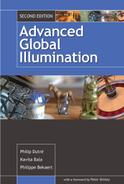
We distinguish four processes: volume emission (Section 8.1.2), absorption (Section 8.1.3), out-scattering (Section 8.1.4), and in-scattering (Section 8.1.5). Figure 8.1 illustrates these processes. This will allow us to generalize the rendering equation of Chapter 2 (Section 8.1.6). Once a good basic understanding of the physics of the problem has been gained, it is quite easy to extend most of the global illumination algorithms previously described in this book to handle participating media (Section 8.1.7).
A participating medium affects radiance transfer along the line from x to y through four processes: absorption (top right) and out-scattering (bottom left) remove radiance; volume emission (top left) and in-scattering (bottom right) add radiance. These processes are explained in more detail in the following sections.
8.1.2 Volume Emission
The intensity by which a medium, like fire, glows can be characterized by a volume emittance function ∊(z) (units [W/m3]). A good way to think about the volume emittance function is as follows: it tells us basically how many photons per unit of volume and per unit of time are emitted at a point z in three-dimensional space. Indeed, there is a close relationship between the number of photons and energy: each photon of a fixed wavelength λ carries an energy quantum equal to 2πħc/λ, where ħ is a fundamental constant in physics, known as Planck’s constant, and c is the speed of light. Of course, the intensity of the glow may vary from point to point in space. Many interesting graphics effects, not only fire, are possible by modeling volume light sources.
Usually, volume emission is isotropic, meaning that the number of photons emitted in any direction around z is equal to ∊(z)/4π (units [W/m3sr]).
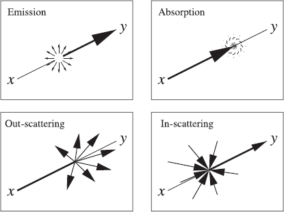
Now consider a point z = x + s · Θ along a thin pencil connecting mutually visible surface points x and y (see Figure 8.2). The radiance added along direction Θ due to volume emission in a pencil slice of infinitesimal thickness ds at z is
dLe(z→Θ)=e(z)4πds. (8.2)
8.1.3 Absorption
Photons traveling along our pencil from x to y will collide with the medium, causing them to be absorbed or change direction (scattering). Absorption means that their energy is converted into a different kind of energy, for instance, kinetic energy of the particles in the medium. Transformation into kinetic energy is observed at a macroscopic level as the medium heating up by radiation. Strong absorption of microwave radiation by water allows you to boil water in a microwave oven.
The probability that a photon gets absorbed in a volume, per unit of distance along its direction of propagation, is called the absorption coefficient σa(z) (units [1/m]). This means that a photon traveling a distance Δs in a medium has a chance σa ∙ Δs of being absorbed. Just like the emission density, the absorption coefficient can also vary from place to place. In cigarette smoke, for example, absorption varies because the number of smoke particles per unit volume varies from place to place. In addition, absorption is usually isotropic: a photon has the same chance of being absorbed regardless of its direction of flight. This is rarely true for absorption by a single particle, but in most media, particles are randomly oriented so that their average directional absorption (and also scattering) characteristics are observed.
Absorption causes the radiance along the thin pencil from x to y to decrease exponentially with distance. Consider a pencil slice of thickness Δs at z = x + sΘ (see Figure 8.2). The number of photons entering the slice at z is proportional to the radiance L(z → Θ) along the pencil. Assuming that the absorption coefficient is equal everywhere in the slice, a fraction σa(z)Δs of these photons will be absorbed. The radiance coming out on the other side of the slice at z + ΔsΘ will be
L(z+Δs⋅Θ→Θ)=L(z→Θ)−L(z→Θ)σa(z)Δs,
or equivalently
L(z+Δs⋅Θ→Θ)−L(z→Θ)Δs=−σa(z)L(z→Θ).
Taking the limit for Δs → 0 yields the following differential equation1:
dL(z→Θ)ds=−σa(z)L(z→Θ) with z = x + sΘ.
In a homogeneous nonscattering and nonemissive medium, the reduced radiance at z along the pencil will be
L(z→Θ)=L(x→Θ)e−σas.
This exponential decrease of radiance with distance is sometimes called Beer’s Law. It is a good model for colored glass, for instance, and has been used for many years in classic ray tracing [170]. If the absorption varies along the considered photon path, Beer’s Law looks like this:
L(z→Θ)=L(x→Θ)exp (−∫s0σa(x+tΘ)dt).
8.1.4 Out-Scattering, Extinction Coefficient, and Albedo
The radiance along the pencil will, in general, not only reduce because of absorption, but also because photons will be scattered into other directions by the particles along their path. The effect of out-scattering is almost identical to that of absorption—one just needs to replace the absorption coefficient by the scattering coefficient σs(z) (units [1/m]), which indicates the probability of scattering per unit of distance along the photon path.
Rather than using σa(z) and σs(z), it is sometimes more convenient to describe the processes in a participating medium by means of the total extinction coefficient σt(z) and the albedo α(z).
The extinction coefficient σt(z) = σa(z) + σs(z) (units [1/m]) gives us the probability per unit distance along the path of flight that a photon collides (absorbs or scatters) with the medium. It allows us to write the reduced radiance at z as
Lr(z→Θ)=L(x→Θ)τ(x,z) with τ(x,z)=exp(−∫rx z0σt(x+tΘ)dt). (8.3)
In a homogeneous medium, the average distance between two subsequent collisions can be shown to be 1/σt (units [m]). The average distance between subsequent collisions is called the mean free path.
The albedo α(z) = σs(z)/σt(z) (dimensionless) describes the relative importance of scattering versus absorption. It gives us the probability that a photon will be scattered rather than absorbed when colliding with the medium at z.
The albedo is the volume equivalent of the reflectivity ρ at surfaces. Note that the extinction coefficient was not needed for describing surface scattering since all photons hitting a surface are supposed to scatter or to be absorbed. In the absence of participating media, one could model the extinction coefficient by means of a Dirac delta function along the photon path: it is zero everywhere, except at the first surface boundary met, where scattering or absorption happens for sure.
8.1.5 In-Scattering, Field-and Volume-Radiance, and the Phase Function
The out-scattered photons change direction and enter different pencils between surface points. In the same way, photons out-scattered from other pencils will enter the pencil between the x and y we are considering. This entry of photons due to scattering is called in-scattering.
Similar to volume emission, the intensity of in-scattering is described by a volume density Lvi(z → Θ) (units [W/m3sr]). The amount of in-scattered radiance in a pencil slice of thickness ds will be
dLi(z→Θ)=Lvi(z→Θ)ds.
A first condition for in-scattering at a location z is that there is scattering at z at all, in other words, that σs(z) = α(z)σt(z) ≠ 0. The amount of in-scattered radiance further depends on the field radiance L(z, Ψ) along other directions Ψ at z, and the phase function p(z, Ψ ↔ Θ).
Field radiance is our usual concept of radiance. It describes the amount of light energy flux in a given direction per unit of solid angle and per unit area perpendicular to that direction. The product of field radiance with the extinction coefficient Lv(z, Ψ) = L(z, Ψ)σt(z) describes the number of photons entering collisions with the medium at z per unit of time. Being a volume density, it is sometimes called the volume radiance (units [1/m3sr]).
Note that the volume radiance will be zero in empty space. The field radiance, however, does not need to be zero and fulfills the law of radiance conservation in empty space.
Note also that for surface scattering, no distinction is needed between field radiance and surface radiance, since all photons interact at a surface.
Of these photons entering collision with the medium at z, a fraction α(z) will be scattered. Unlike emission and absorption, scattering is usually not isotropic. Photons may scatter with higher intensity in certain directions than in others. The phase function p(z, Ψ ↔ Θ) at z (units [1/sr]) describes the probability of scattering from direction Ψ into Θ. Usually, the phase function only depends on the angle between the two directions Ψ and Θ. Some examples of phase functions are given below.
The product α(z)p(z, Ψ ↔ Θ) plays the role of the BSDF for volume scattering. Just like BSDFs, it is reciprocal, and energy conservation must be satisfied. It is convenient to normalize the phase function so that its integral over all possible directions is one:
∫Ωp(z,Ψ↔Θ)dωΨ=1.
Energy conservation is then clearly satisfied, since α(z) < 1.
Putting this together, we arrive at the following volume scattering equation:
L υi(z→Θ)=∫Ωα(z)p(z, Ψ↔Θ)⋅L υ(z→Ψ)dωΨ =σs(z)∫Ωp(z, Ψ↔Θ)L(z→Ψ)dωΨ.(8.4)
The volume scattering equation is the volume equivalent of the surface scattering equation introduced in Section 2.5.1. It describes how scattered volume radiance is the integral over all directions of the volume radiance Lv(z → Ψ), weighted with α(z)p(z, Ψ ↔ Θ). The former is the volume equivalent of surface radiance, and the latter is the equivalent of the BSDF.
Examples of Phase Functions
The equivalent of diffuse reflection is called isotropic scattering. The phase function for isotropic scattering is constant and equal to
p(z,Ψ↔Θ)=14π. (8.5)
An often used nonisotropic phase function is the following Henyey-Greenstein phase function, which was introduced to model light scattering in clouds:
p(z,Ψ↔Θ)=14π1−g21+g2−2g cos(Ψ, Θ)3/2. (8.6)
The parameter g allows us to control the anisotropy of the model: it is the average cosine of the scattering angle. With g > 0, particles are scattered with preference in forward directions. With g < 0, they are scattered mainly backward. g = 0 models isotropic scattering (see Figure 8.3).

Polar plots of the Henyey-Greenstein phase function for anisotropy parameter value g = 0.0 (isotropic, left), g = −0.2, −0.5, −0.9 (dominant backward scattering, top row), and g = +0.2, +0.5, +0.9 (dominant forward scattering, bottom row). These plots show the intensity of scattering as a function of the angle between forward and scattered direction.
Other common nonisotropic phase functions are due to Lord Rayleigh and Blasi et al. Rayleigh’s phase function [22, Chapter 1] describes light scattering at very small particles, such as air molecules. It explains why a clear sky is blue above and more yellow-reddish towards the horizon.
Blasi et al. have proposed a simple-to-use, intuitive, and efficient-to-evaluate phase function for use in computer graphics [17].
8.1.6 The Rendering Equation in the Presence of Participating Media
We are now ready to describe how the radiance L(x → Θ) gets modified along its way to y. Equation 8.2 and Equation 8.4 model how volume emission and in-scattering add radiance along a ray from x to y. Equation 8.3, on the other hand, describes how radiance is reduced due to absorption and out-scattering. Not only the surface radiance L(x → Θ) inserted into the pencil at x is reduced in this way, but also all radiance inserted along the pencil due to in-scattering and volume emission is reduced. The combined effect is
L(y←−Θ)=L(x→Θ)τ(x,y)+∫rxy0L+(z→Θ)τ(z,y)dr. (8.7)
For compactness, we let z = x + rΘ and
L+(z→Θ)=ε(z)/4π+Lvi(z→Θ) (units [W/m3sr]).
The transmittance τ(z, y) indicates how radiance is attenuated between z and y:
τ(z,y)=exp(−∫rzy0σt(z+sΘ)ds). (8.8)
Equation 8.7 replaces the law of radiance conservation (Equation 8.1) in the presence of participating media.
Recall that the rendering equation in Chapter 2 was obtained by using the law of radiance conservation in order to replace the incoming radiance L(x ← Ψ) in
L(x→Θ)=Le(x→Θ)+∫Ωfr(x,Θ↔Ψ)L(x←Ψ)cos(Ψ,Nx)dωΨ
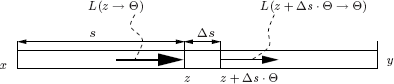
by the outgoing radiance L(y → −Ψ) at the first surface point y seen from x in the direction Ψ. Doing a similar substitution here, using Equation 8.7 instead, yields the following rendering equation in the presence of participating media (see Figure 8.4):
L(x→Θ)=Le(x→Θ) +∫ΩL(y→−Ψ)τ(x,y)fr(x,Θ↔Ψ)cos (Ψ,Nx)dωΨ +∫Ω(∫rxxy0L+(z→−Ψ)τ(z,y)dr)fr(x,Θ↔Ψ)cos (Ψ,Nx)dωΨ. (8.9)
The in-scattered radiance Lvi in L+(z → −Ψ) = є(z)/4π + Lvi(z → −Ψ) is expressed in terms of field radiance by Equation 8.4. In turn, field radiance is expressed in terms of surface radiance and volume emitted and in-scattered radiance elsewhere in the volume by Equation 8.7.
These expressions look much more frightening than they actually are. The important thing to remember is that participating media can be handled by extending the rendering equation in two ways:
- Attenuation of radiance received from other surfaces: the factor τ(x, y) given by Equation 8.8 in the former integral.
- A volume contribution: the latter (double) integral in Equation 8.9.
Spatial Formulation
In order to better understand how to trace photon trajectories in the presence of participating media, it is instructive to transform the integrals above to a surface and volume integral, respectively. The relation r2xy dωΨ=V(x, y) cos(–Ψ, Ny)dAy between differential solid angle and surface was derived in Section 2.6.2. A similar relationship exists between drdωΨ and differential volume: r2xz drdωΨ=V(x, z) dVz. This results in
L(x→Θ)=Le(x→Θ) +∫Sfr(x, Θ↔Ψ)L(y→–Ψ)τ(x, y)V(x, y)cos(Ψ, Nx) cos(–Ψ, Ny)r2xydAy +∫Vfr(x, Θ↔Ψ)L +(z→–Ψ)τ(x, y)V(x, z)cos(Ψ, Nx)r2xzdVz. (8.10)
The two integrands are very similar: the volume integral contains L+(z →−Ψ) [W/m3sr] rather than surface radiance L(y → −Ψ) [W/m2sr], but also, surface points always come with a cosine factor, while volume points don’t.
The correspondences and differences between volume and surface scattering quantities and concepts are summarized in Figure 8.5.
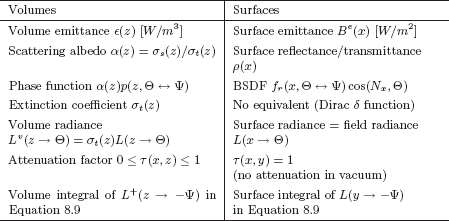
This table summarizes the main correspondences and differences in volume and surface scattering and emission.
8.1.7 Global Illumination Algorithms for Participating Media
Rendering participating media has received quite some attention since the end of the 1980s. Proposed approaches include deterministic methods and stochastic methods. Classic and hierarchical radiosity methods have been extended to handle participating media by discretizing the volume integral above into volume elements and assuming that the radiance in each volume element is isotropic [154, 174]. Many other deterministic approaches have been proposed as well, based on spherical harmonics (PN methods) and discrete ordinates methods. An overview is given in [143]. Deterministic approaches are valuable in relatively “easy” settings, for instance, homogeneous media with isotropic scattering, or simple geometries.
Various authors, including Rushmeier, Hanrahan, and Pattanaik, have proposed extensions to path tracing to handle participating media. These extensions have been used for some time in other fields such as neutron transport [183, 86]. They are summarized in Section 8.1.8. The extension of bidirectional path tracing to handle participating media has been proposed in [104]. As usual, these path-tracing approaches are flexible and accurate, but they become enormously costly in optically thick media, where photons suffer many collisions and trajectories are long.
A good compromise between accuracy and speed is offered by volume photon density estimation methods. In particular, the extension of photon mapping to participating media [78] is a reliable and affordable method capable of rendering highly advanced effects such as volume caustics. Volume photon density estimation is described in more detail in Section 8.1.9.
Monte Carlo and volume photon density estimation are methods of choice for optically thin media, in which photons undergo only relatively few collisions. For optically thick media, they become intractable. Highly scattering optically thick media can be handled with the diffusion approximation, covered concisely in Section 8.1.10.
For the special case of light scattering and attenuation in the Earth’s atmosphere, an analytical model has been proposed [148]. It plausibly reproduces the color variations of the sky as a function of sun position and adds great realism to outdoor scenes without costly simulations.
Figure 8.6 shows some example renderings of participating media using techniques covered here.
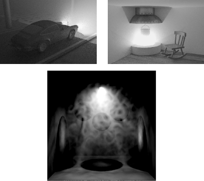
Some renderings of participating media. The top images have been rendered with bidirectional path tracing.
(Courtesy of Eric Lafortune, Katholieke Universiteit Leuven, Belgium.) The bottom image was rendered with volume photon mapping. Note the volume caustics cast on this inhomogeneous medium behind the colored spheres. (Courtesy of Frederik Anrys and Karl Vom Berge, Katholieke Universiteit Leuven, Belgium.) (See Plate XI.).
8.1.8 Tracing Photon Trajectories in Participating Media
Most algorithms discussed so far in this book are based on the simulation of the trajectory of photons or potons, potential particles originating at the eye rather than at light sources. We discuss here how to extend photon- or poton-trajectory tracing to deal with participating media.
Sampling volume emission. Light particles may not only be emitted at surfaces, but also in midspace. First, a decision needs to be made whether to sample surface emission or volume emission. This decision can be a random decision based on the relative amount of self-emitted power by surfaces and volumes, for instance. If volume emission is to be sampled, a location somewhere in midspace needs to be selected, based on the volume emission density є(z): bright spots in the participating media shall give birth to more photons than dim regions. Finally, a direction needs to be sampled at the chosen location. Since volume emission is usually isotropic, a direction can be sampled with uniform probability across a sphere. Just like with surface emission sampling, this is a spatial position and a direction result.
Sampling a next collision location. In the absence of participating media, a photon emitted from point x into direction Θ always collides on the first surface seen from x along the direction Θ. With participating media, however, scattering and absorption may also happen at every location in the volume along a line to the first surface hit. Note that both surface and volume collisions may take place, regardless of whether x is a surface or a volume point. A good way to handle this problem is to sample a distance along the ray from x into Θ, based on the transmittance factor (Equation 8.8). For instance, one draws a uniformly distributed random number ζ ∈ [0, 1) (including 0, excluding 1) and finds the distance r corresponding to
exp(−∫r0σt(x+sΘ)ds)=1−ζ ⇔ ∫r0σt(x+sΘ)ds=−log(1−ζ).
In a homogeneous medium, r = — log(1 — ζ)/σt. In a heterogeneous medium, however, sampling such a distance is less trivial. It can be done exactly if the extinction coefficient is given as a voxel grid, by extending ray-grid traversal algorithms. For procedurally generated media, one can step along the ray in small, possibly adaptively chosen, intervals [78]. If the selected distance becomes greater than or equal to the distance to the first surface hit point of the ray, surface scattering shall be selected as the next event. If the sampled distance is nearer, volume scattering is chosen (see Figure 8.7).
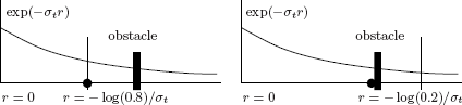
Sampling a next photon collision location along a ray. First, a distance r is sampled using the attenuation τ(x, z) as a PDF (τ (x, z) = exp(—σtrxz) in a homogeneous medium). If this distance is less than the distance to the nearest surface (left), then volume scattering or absorption is chosen as the next event. If r is further than the nearest surface (right), surface absorption or scattering is selected at the nearest surface.
Sampling scattering or absorption. Sampling scattering or absorption in a volume is pretty much the same as for surfaces. The decision whether to scatter or absorb will be based on the albedo α(z) for volumes just like the reflectivity ρ(z) is used for surfaces. Sampling a scattered direction is done by sampling the phase function p(z, Θ ↔ Ψ) for volumes. For surfaces, one ideally uses fr(z, Θ ↔ Ψ) cos(Nx, Ψ)/ρ(z).
Connecting path vertices. Algorithms such as path tracing and bidirectional path tracing require us to connect path vertices, for instance, a surface or volume hit with a light source position for a shadow ray. Without participating media, the contribution associated with such a connection between points x and y is
V(x,y)cos(Nx, Θ)cos(Ny, −Θ)r2xy.
In the presence of participating media, the contribution shall be
τ(x,y)V(x, y)r2xyCx(Θ)Cy(−Θ),
with Cx(Θ) = cos(Nx, Θ) if x is a surface point or 1 if it is a volume point (similarly for Cy(—Θ)).
8.1.9 Volume Photon Density Estimation
The photon density estimation algorithms of Section 6.5 computed radiosity on surfaces by estimating the density of photon hit points on surfaces. In order to render participating media, it is also necessary to estimate the volume density of photons colliding with the medium in midspace. Any of the techniques described in Section 6.5 can be extended for this purpose in a straightforward manner. A histogram method, for instance, would discretize the space into volume bins and count photon collisions in each bin. The ratio of the number of photon hits over the volume of the bin is an estimate for the volume radiance in the bin. Photon mapping has been extended with a volume photon map, a third kd-tree for storing photon hit points, in the same spirit as the caustic and global photon map discussed in Section 7.6 [78]. The volume photon map contains the photons that collide with the medium in midspace. Rather than finding the smallest disc containing a given number N of photon hit points, as was done on surfaces, one will search for the smallest sphere containing volume photons around a query location. Again, the ratio of the number of photons and the volume of the sphere yields an estimate for the volume radiance.
Viewing Precomputed Illumination in Participating Media
Due to the law of conservation of radiance, viewing precomputed illumination using ray tracing in the absence of participating media takes nothing more than finding what surface point y is visible through each pixel on the virtual screen and querying the illumination at that point.
In the presence of participating media, conservation of radiance does not hold, and the radiance coming in at the observer through each pixel will be an integral over an eye ray, according to Equation 8.7. A good way to evaluate this integral is by ray marching [78]: by stepping over the ray in small, potentially adaptively chosen, intervals (see Figure 8.8). At every visited location along the ray, precomputed volume radiance is queried, and volume emission and single scattered radiance evaluated. Of course, the surface radiance at the first hit object should not be overlooked. All radiance contributions are appropriately attenuated towards the eye.
Using precomputed volume radiance for rendering a view can best be done with a technique called ray marching. One marches over an eye ray, with fixed or adaptive step size. At every step, precomputed volume radiance is queried. Self-emitted and single scattered (“direct”) volume radiance is calculated on the spot. Finally, the surface radiance at the first hit surface is taken into account. All gathered radiance is properly attenuated.
8.1.10 Light Transport as a Diffusion Process
The rendering equation (Equation 8.9) is not the only way light transport can be described mathematically. An interesting alternative is to consider the flow of light energy as a diffusion process [75, Chapter 9]. This point of view has been shown to result in efficient algorithms for dealing with highly scattering optically thick participating media, such as clouds [185]. The diffusion approximation is also at the basis of recently proposed models for subsurface scattering [80]; see Section 8.1.11. We present it briefly here.
The idea is to split field radiance in a participating media into two contributions, which are computed separately:
L(x→Θ)=Lr(x→Θ)+Ld(x→Θ).
The first part, Lr(x → Θ), called reduced radiance, is the radiance that reaches point x directly from a light source, or from the boundary of the participating medium. It is given by Equation 8.7 and needs to be computed first.
The second part, Ld(x → Θ), is radiance scattered one or more times in the medium. It is called diffuse radiance. In a highly scattering optically thick medium, the computation of diffuse radiance is hard to do according to the rendering equation (Equation 8.9). Multiple scattering, however, tends to smear out the angular dependence of diffuse radiance. Indeed, each time a photon scatters in the medium, its direction is randomly changed as dictated by the phase function. After many scattering events, the probability of finding the photon traveling in any direction will be nearly uniform.
For this reason, one approximates diffuse radiance by the following function, which varies only a little with direction:
Ld(x→Θ)=Ud(x)+34π(→Fd(x)⋅Θ).
Ud(x) represents the average diffuse radiance at x:
Ud(x)=14π∫ΩLd(x,Θ)dωΘ.
The vector →Fd(x), called the diffuse flux vector, models the direction and magnitude of the multiple-scattered light energy flow through x. It is defined by taking Θ equal to the unit vector in X, Y, and Z directions in the following equation:
(→Fd(x)⋅Θ)=∫ΩL(x→Ψ) cos(Ψ, Θ)dωΨ.
In this approximation, it can be shown that the average diffuse radiance Ud fulfills a so-called steady-state diffusion equation:
∇2Ud(x)−σ2trUd(x)=−Q(x). (8.11)
The driving term Q(x) can be computed from reduced radiance [185, 80, 75, Chapter 9]. The diffusion constant equals σ2tr=3σaσ′t with σ′t = σ′s + σa and σ′s = σs(1 — g). g is the average scattering cosine (see Section 8.1.5) and models the anisotropy of scattering in the medium.
Once the diffusion equation has been solved, the reduced radiance and the gradient of Ud(x) allow us to compute the flux vector →Fd(x) wherever it is needed. The flux vector, in turn, yields the radiosity flowing through any given real or imaginary surface boundary.
For simple cases, such as a point source in an infinite homogeneous medium, the diffusion equation can be solved analytically [80, 75, Chapter 9]. In general, however, solution is only possible via numerical methods. Stam proposed a multigrid finite difference method and a finite element method based on blobs [185]. In any case, proper boundary conditions need to be taken into account, enforcing that the net influx of diffuse radiance at the boundary is zero (because there is no volume scattering outside the medium).
A different alternative for the rendering equation, based on principles of invariance [22], has been described in [145]. It is, however, significantly more involved.
8.1.11 Subsurface Scattering
In the derivation of the rendering equation (Chapter 2), it was also assumed that light hitting an object surface is reflected or refracted from the spot of incidence. This assumption is not always true. Consider, for instance, the small marble horse sculpture in Figure 8.9. Marble, but also other materials including fruits, leaves, candle wax, milk, human skin, etc., are translucent materials. Photons hitting such materials will enter the object, scatter below the surface, and emerge at a different place (see Figure 8.10). Because of this, such materials have a distinct, soft appearance. Figure 8.9 illustrates that a BRDF, which models only local light reflection, cannot capture this soft appearance.
![Figure showing two renderings of a small marble horse sculpture (5 cm head-to-tail). Left: using a BRDF model; right: taking into account subsurface scattering. A BRDF does not capture the distinct, soft appearance of materials such as marble. The right figure has been computed using the model and the path-tracing extension proposed in [80]. These images also illustrate that translucency is an important visual cue for estimating the size of objects.](http://imgdetail.ebookreading.net/software_development/6/9781439864951/9781439864951__advanced-global-illumination__9781439864951__image__270x001.png)
Two renderings of a small marble horse sculpture (5 cm head-to-tail). Left: using a BRDF model; right: taking into account subsurface scattering. A BRDF does not capture the distinct, soft appearance of materials such as marble. The right figure has been computed using the model and the path-tracing extension proposed in [80]. These images also illustrate that translucency is an important visual cue for estimating the size of objects.
(See Plate XII.).

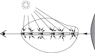
Subsurface scattering. Photons entering a translucent material will undergo a potentially very large number of scattering events before they reappear at a different location on the surface.
In principle, translucency can be handled using any of the previously discussed algorithms for participating media. Materials such as marble and milk are, however, highly scattering and optically thick. A photon entering a marble object for instance, will scatter hundreds of times before being absorbed or reappearing at the surface. Algorithms based on photon trajectory tracing are very inefficient in this case. The diffusion approximation, however, can be used.
Translucency can also be treated in a more macroscopic way, by extending the model for light reflection introduced in Section 2.5.1, so that light can reflect off a different location than where it entered the material:
L(y→Θ)=∫s∫Ω+xL(x←Ψ)S(x,Ψ↔y,Θ)cos(Nx,Ψ)dωΨdAx. (8.12)
The function S(x, Ψ ↔ y, Θ) is called the bidirectional surface scattering reflectance distribution function (BSSRDF, units [1/m2sr]). It depends on two surface positions rather than one, but other than that it plays exactly the same role, and has a similar meaning as the BRDF.
Practical models for the BSSRDF have been proposed by Hanrahan et al. [63] and Jensen et al. [80]. The former model is based on an analytic solution of the rendering equation (Equation 8.9) in a planar slab of a homogeneous medium, taking into account only single scattering. The latter model is based on an approximate analytic solution of the diffusion equation (Equation 8.11) in an infinitely thick planar slab filled with a homogeneous medium. It looks like this:
S(x, Θ↔y, Ψ) = 1πFt(η, Θ)Rd(x, y)Ft(η, Ψ) Rd(x, y) = α′4π[zr(1+σtrdr)e–σtrdrd3r+(1+σtrdυ)e–σtrdυd3υ] . (8.13)
Ft(η, Θ) and Ft(η, Ψ) denote the Fresnel transmittance for incident/ outgoing directions Θ at x and ψ at y (see Section 2.8). The parameters η (relative index of refraction), α′ = σ′s/σ′t, and σtr=√3σaσ′t are material properties (σ′s, σ′t, and σtr were introduced in Section 8.1.10). zr and zv are the distance a pair of imaginary point sources are placed above and below x (see Figure 8.11). dr and dv are the distance between y and these source points. zr and zv are to be calculated from the material parameters [80]. Jensen et al. also proposed practical methods for determining the material constants σa and σ′s, and they give values for several interesting materials like marble and human skin [80, 76].
![Figure showing jensen BSSRDF model is based on a dipole source approximation: A pair of imaginary point sources sr and sv are placed one above and one below the surface point x. The distance zr and zv at which these sources are placed with regard to x are calculated from the reduced scattering coefficient σ’s and the absorption coefficient σa of the medium inside the object (see [80]). The BSSRDF model further depends on the distance dr and dv between a surface point y and these point sources. The graphs at the bottom show the diffuse reflectance due to subsurface scattering Rd for a measured sample of marble using parameters from [80]. Rd(r) indicates the radiosity at a distance r [mm] in a plane, due to unit incident power at the origin. The graphs illustrate that subsurface scattering is significant up to a distance of several millimeters in marble. The graphs also explain the strong color filtering effects observed at larger distances. The right image in Figure 8.9 was computed using this model.](http://imgdetail.ebookreading.net/software_development/6/9781439864951/9781439864951__advanced-global-illumination__9781439864951__image__272x001.png)
Jensen BSSRDF model is based on a dipole source approximation: A pair of imaginary point sources sr and sv are placed one above and one below the surface point x. The distance zr and zv at which these sources are placed with regard to x are calculated from the reduced scattering coefficient σ’s and the absorption coefficient σa of the medium inside the object (see [80]). The BSSRDF model further depends on the distance dr and dv between a surface point y and these point sources.
The graphs at the bottom show the diffuse reflectance due to subsurface scattering Rd for a measured sample of marble using parameters from [80]. Rd(r) indicates the radiosity at a distance r [mm] in a plane, due to unit incident power at the origin. The graphs illustrate that subsurface scattering is significant up to a distance of several millimeters in marble. The graphs also explain the strong color filtering effects observed at larger distances. The right image in Figure 8.9 was computed using this model.
Several algorithms have been proposed for rendering images with this BSSRDF model. In path-tracing and similar algorithms, computing direct illumination at a point x on a translucent object takes tracing a shadow ray at a randomly sampled other location y on the object surface, rather than at x [80]. The factor Rd(x, y) = Rd(r) in Equation 8.13 at the heart of Jensen’s model depends only on the distance r between points x and y. Rd(r) can be used as a PDF for sampling a distance r. The point y is then chosen on the object surface, at this distance r from x. The right image in Figure 8.9 was rendered in this way.
The extension to full global illumination with algorithms such as photon mapping has been proposed in [76]. In [109], a radiosity-like approach can be found, which allows us to interactively change viewing and lighting conditions after some preprocessing.
8.1.12 Polarization, Interference, Diffraction, Fluorescence, Phosphorescence and Nonconstant Media
So far in this chapter, we have discussed how to extend the rendering equation in order to deal with participating media and nonlocal light reflection. Here, we cover how some more approximations made in Chapter 2 can be overcome.
Nonconstant Media: Mirages and Twinkling Stars and Such
The assumption that light travels along straight lines is not always true. Gradual changes in the index of refraction of the medium cause light rays to bend. Temperature changes in the earth’s atmosphere, for instance, affect the index of refraction and cause midair reflections such as mirages. Another example is the twinkling of stars in a clear, but turbulent, night sky. Several efficient techniques to trace rays in such nonconstant media can be found in [184].
Fluorescence and Phosphorescence: Reflection at a Different Wavelength and a Different Time
We assumed that reflected light has the same wavelength as incident light and that scattering is instantaneous. This allows us to solve the rendering equation independently and in parallel for different wavelengths, and at different time instances.
Some materials, however, absorb electromagnetic radiation to reradiate it at a different wavelength. For instance, ultraviolet or infrared radiation can be reradiated as visible light. If reradiation happens (almost) immediately, such materials are called fluorescent materials. Examples of fluorescent objects include fluorescent light bulbs, Post-It notes, and certain detergents that “wash whiter than white.”
Other materials reradiate only at a significantly later time. Such materials are called phosphorescent materials. Phosphorescent materials sometimes store light energy for hours. Some examples are the dials of certain wrist watches and small figures, such as decorations for children’s bedrooms, that reradiate at night the illumination captured during the day.
Fluorescence and phosphorescence can be dealt with by extending the BRDF to a matrix, describing cross-over between different wavelengths in scattering. Delay effects in phosphorescence can be modeled adequately by extending the notion of self-emitted radiation, keeping track of incident illumination in the past [53, 226].
Interference: Soap Bubbles and Such
When two waves of the same frequency meet at some place, they will cancel or amplify each other depending on their phase difference. This effect is called interference and can be observed, for instance, in water surface waves in a (not too crowded) swimming pool. Electromagnetic radiation, and thus light, also has wave properties (see Section 2.1) and may suffer from interference. Interference of radio waves, for instance, due to two radio stations broadcasting at the same shortwave frequency, is very well known to radio amateurs and causes an effect sometimes called the Mexican dog. Interference of light waves can be observed in reflections at transparent thin films, and causes a colorful effect called Newton rings. This happens, for instance, in soap bubbles or gas spills on the road.
Interference is explained by addition of wave amplitudes, taking into account wave phase correctly. The transport theory of electromagnetic radiation, which leads to the rendering equation, is based on the addition of power, rather than amplitudes, and ignores phase effects. It is, however, possible to extend ray tracing to take phase effects into account. Gondek et al. [55] have used such a ray tracer as a virtual gonio-reflectometer to calculate BRDFs that are capable of reproducing interference effects (see Figure 8.12).

Interference of light at a transparent thin film coating causes colorful reflections on these sunglasses. The BRDF model used for rendering this image has been calculated using a wave-phase–aware ray tracer.
(Image courtesy of Jay Gondek, Gary Meyer, and John Newman, University of Oregon.) (See Plate XIII.)
Diffraction: Compact Discs and Brushed Metals
Diffraction is the cause of other colorful light-scattering effects, such as at the surface of a compact disc or brushed metals. Diffraction can be viewed as interference of coherent secondary spherical waves originating at nearby locations. It is observed when light is scattered at surface features with size comparable to the wavelength of light (around 0.5 micrometers). The holes on a CD-ROM surface, for instance, are of this size. They are also regularly spaced so that they form a so-called diffraction grating. Since diffraction is a wave effect as well, it is not accounted for in the transport theory of light. Diffraction observed in reflections at certain rough surfaces can be modeled by means of an appropriate BRDF [186]. Figure 8.13 shows an image rendered with such a diffraction shader.

The colorful reflections on this CD-ROM are caused by diffraction. Like other effects due to the wave nature of light, diffraction is not accounted for in the transport theory of light. Diffraction in reflections at certain rough surfaces can, however, be incorporated in a BRDF model.
(Image courtesy of Jos Stam, Alias|Wavefront.) (See Plate XIV.).
Polarization
Polarization of light is an effect well known to outdoor photographers, who use polarization filters to make the sky appear more pure in their pictures. It can play an important role whenever multiple specular reflections and refractions occur at smooth surfaces. Examples are optical instruments, multifaceted crystal objects, and gemstones.
Polarization can be explained by considering electromagnetic radiation as a superposition of two transverse waves, which oscillate in directions perpendicular to each other and to the direction of propagation.
Often, there is no correlation between the phases of these waves, so that average properties are observed. Such light is called unpolarized or natural light. Most light sources emit natural light. Light usually becomes polarized due to scattering. The Fresnel equations (Section 2.8), for instance, demonstrate how the two components reflect and refract with different intensities at smooth surface boundaries. Rayleigh’s phase function [22, Chapter 1] models how light scattered at air molecules gets polarized. Outdoor photographers take advantage of the latter.
In order to describe the polarization state of light completely, four parameters are needed. Often in optics literature, amplitude and phase correlation functions of the two component waves are used. In transport theory, it is more convenient to use a different parametrization, due to Stokes (see, for instance, [75, Chapter 7] and [22, Chapter 1]).
From the point of view of a global illumination practitioner, the main issue is that polarized light is characterized by four radiance functions, rather than just one. Surface and volume scattering is described by a 4 × 4 matrix of BSDF or phase functions that model the cross-over between any of the four radiance components before and after scattering. Wilkie et al. [226] have implemented this in a stochastic ray tracer. Some of their renderings are reproduced in Figure 8.14.

These images illustrate polarization of light reflected in the glass block on the left (Fresnel reflection). The same scene is shown, but with a different filter in front of the virtual camera: a horizontal polarization filter (left), vertical polarization filter (middle); and a 50% neutral gray (nonpolarizing) filter (right).
(Image courtesy of A. Wilkie, Vienna University of Technology, Austria.) (See Plate XV.)
8.2 Image Display and Human Perception
Most of the discussion in this book so far has focused on computing the correct radiometric values for each pixel in the final image. These values are measured in radiance, which expresses the amount of energy per surface area per solid angle that can be measured at a specific point in space and in a specific direction. However, these physically based radiance values do not adequately express how brightly the human eye perceives different illumination levels. The human visual system does not respond linearly to changing levels of illumination. By knowing how the human visual system reacts to light incident on the eye’s receptors, aspects such as the display of images or the computation of the light transport distribution can be improved.
A global illumination solution for a typical scene might contain many different levels of illumination. The most typical example is a scene in which the sun is present. This very bright light source has a radiance level much higher than any other surface in the scene (except for perhaps other artificial, unnatural light sources that might be present). For some scenes, the ratio between the lowest and highest radiance levels could be as high as 105. Figure 8.16 shows a logarithmic plot of the environment map shown in Figure 8.15, and 5 orders of magnitude are present in this picture. The same scene rendered by daylight, artificial light, or lit by a night sky might also yield very different levels of illumination. Typical luminance levels vary from 10—3 candela per square meter for starlight to 105 candela per square meter for bright sunlight. It is therefore important to design procedures that can map these different intensity ranges on the desired output device, while preserving the perceived realism of the high intensity ratios present in the radiometrically accurate image.

Various tone-mapping operators. (a) Linear scaling; (b) gamma scaling; (c) simple model of lightness sensitivity; (d) complex model for the human visual system.
(See Plate XVI.)
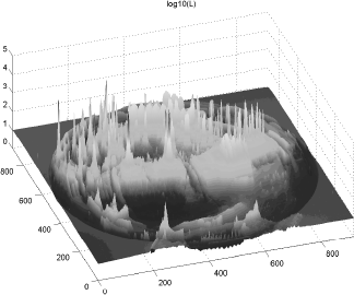
Luminance values for the high dynamic range photograph of an environment reflected in a scene shown in Figure 8.15.
As we all experience every day, the human eye can quickly adapt to such varied levels of illumination. For example, we might be in a dark room and see the features of the room, and at the same time see the brightly lit scene outdoors when looking through the window. Car drivers can adapt quickly from darkness to sunlight when exiting a tunnel or vice versa. This process is known as visual adaptation. Different mechanism are responsible for the visual adaption of the human eye:
- Receptor types. There are two types of receptors in the human retina, named after their respective shapes: cones and rods. The cone receptors are mostly sensitive to color and bright illumination; the rods are sensitive to vision in the lower illumination ranges. By having two types of receptors being sensitive to different illumination conditions, the human visual system is able to adapt between various levels of illumination.
- Photopigment bleaching. When a receptor reacts to incident light, bright light might make the receptor less sensitive. However, this loss of sensitivity is restored after a short period of time, when the receptor has adapted to the new illumination level.
- Neural mechanisms. Most visual neurons respond linearly within only a very narrow band of the entire range of incoming illumination.
Visual adaptation is also highly dependent on the background illumination intensity. When exposed to a high background illumination, the photoreceptors become saturated and lose their sensitivity to any further increments of the intensity. However, after some time, the response gradually returns to its former levels, and the sensitivity returns to its previous levels. As such, the level of background illumination, or the adaptation luminance, is an important factor in defining the state of the visual adaption.
All these factors have been acquired by experimental data. There is a large amount of psychophysical data available, quantifying the performance of the human visual system under different conditions.
8.2.1 Tone Mapping
Tone-mapping operators solve the problem of how to display a high dynamic range picture on a display device that has a much lower range of available displayable intensities. For example, a typical monitor can display only luminance values from 0.1 up to 200 cd/m2. Depending on the type of monitor, the dynamic range (the ratio between the highest and lowest possible emitted intensities) can be 1 : 1000 to 1 : 2000; although with the introduction of new high-dynamic range display technology, this ratio is steadily growing. Mapping the vast range of luminance values that can be present in high dynamic range images to this very limited display range therefore has to be carried out accurately in order to maintain the perceptual characteristics of the image, such that a human observer receives the same visual stimuli when looking at the original image or at the displayed image.
A very simple solution for displaying the different illumination ranges in the image is by linearly scaling the intensity range of the image into the intensity range of the display device. This is equivalent to setting the exposure of a camera by adjusting the aperture or shutter speed, and results in the image being shown as if it would have been photographed with these particular settings. This, however, is not a viable solution, since either bright areas will be visible and dark areas will be underexposed, or dark areas will be visible and the bright areas will be overexposed. Even if the dynamic range of the image falls within the limits of the display, two images that only differ in their illumination levels by a single scale factor will still map to the same display image due to the simple linear scaling. It is therefore possible that a virtual scene illuminated by bright sunlight will produce the same image on the display compared to the same scene illuminated by moonlight or starlight. Rather, effects such as differences in color perception and visual acuity, which change with various levels of illumination, should be maintained.
A tone-mapping operator has to work in a more optimal way than just a linear scaling, by exploiting the limitations of the human visual system in order to display a high dynamic range image. Generally, tone-mapping operators create a scale factor for each pixel in the image. This scale factor is based on the local adaptation luminance of the pixel, together with the high dynamic range value of the pixel. The result is typically an RGB value that can be displayed on the output device. Different tone-reproduction operators differ in how they compute this local adaptation luminance for each pixel. Usually, an average value is computed in a window around each pixel, but some algorithms translate these computations to the vertices present in the scene.
Different operators can be classified in various categories [74]:
- Tone-mapping operators can be global or local. A global operator uses the same mapping function for all pixels in an image, as opposed to a local operator, where the mapping function can be different for each pixel or group of pixels in the image. Global operators are usually inexpensive to compute but do not always handle large dynamic range ratios very well. Local operators allow for better contrast reduction and therefore a better compression of the dynamic range, but they can introduce artifacts in the final image such as contrast reversal, resulting in halos near high contrast edges.
- A second distinction can be made between empirical and perceptually based operators. Empirical operators try to strive for effects such as detail preservation, avoidance of artifacts, or compression of the dynamic range. Perceptually based operators try to generate images that look perceptually the same as the real scene when observed by the human visual system. These operators take into account effects such as the loss of visual acuity or color sensitivity under different illumination levels.
- A last distinction can be made between static or dynamic operators, depending on whether one wants to map still images only or a video sequence of moving images. Time-coherency obviously is an important part of a dynamic operator. Effects such as sudden changes from dim to bright environments (the classic example being a car driver entering or leaving a tunnel) can be modeled with these dynamic operators.
Commonly used tone-mapping operators include the following:
- The Tumblin-Rushmeier tone-mapping operator [199] was the first to be used in computer graphics. This operator preserves the perceived brightness in the scene by trying to match the perceived brightness of a certain area in the image to the brightness of the same area on the output display. It behaves well when brightness changes are large and well above the threshold at which differences in brightness can be perceived.
- The tone-mapping operator developed by Ward [222] preserves threshold visibility and contrast, rather than brightness, as is the case in the Tumblin-Rushmeier operator. This technique preserves the visibility at the threshold of perception (see also the TVI function below). A similar operator was developed by Ferwerda et al. [47] that also preserves contrast and threshold visibility but at the same time tries to reproduce the perceived changes in colors and visual acuity under different illumination conditions.
- Ward [51] also has developed a histogram-based technique that works by redistributing local adaptation values such that a monotonic mapping utilizing the whole range of display luminance is achieved. This technique is somewhat different from previous approaches, in that the adaptation luminance is not directly used to compute a scale factor. Rather, all adaptation and luminance values are used to construct a mapping function from scene luminance to display luminance values.
- Several time-dependent tone operators [141] that take into account the time-dependency of the visual adaptation have also been developed, such that effects such as experiencing a bright flash when walking from a dark room into the bright sunlight can be simulated. These operators explicitly model the process of bleaching, which is mainly responsible for these changing effects due to the time-dependency of the visual adaptation level.
Figure 8.15 shows the result of applying some tone-mapping operators on a high dynamic range picture of an environment reflected in a sphere, of which the actual luminance values are plotted in Figure 8.16. Figure 8.15(a) shows the resulting image when the original high dynamic range picture is scaled linearly to fit into the luminance range of the display device. Figure 8.15(b) applies a simple gamma scaling, in which the displayed intensity is proportional to Luminance1/γ. Figure 8.15(c) uses a simple approximation of the sensitivity to lightness of the human eye, by making the displayed values proportional to 3√Lum/Lumref, with Lumref proportional to the average luminance in the scene, such that the average luminance would be displayed at half the intensity of the display. This model preserves saturation at the expense of image contrast. Figure 8.15(d) uses a more complicated model of the human visual system (Ward’s histogram method), incorporating some of the factors described above.
Research into tone-mapping operators is still continuing, making use of new understanding of how the human visual system perceives images, and driven by the availability of new display technology. A good overview of various operators can be found in [37]. In [108], an evaluation of various tone-mapping operators using a high dynamic range display is presented, using user studies to determine what operators operate best under different conditions.
8.2.2 Perception-Based Acceleration Techniques
Knowledge of the human visual system cannot only be used to design tone-mapping operators but can also help to accelerate the global illumination computations themselves. As an example, consider that the ability to detect changes in illumination drops with increasing spatial frequency and speed of movement. Thus, if these factors are known, it is possible to compute a margin within which errors in the computed illumination values can be tolerated without producing a noticeable effect in the final images. From a physical point of view, these are errors tolerated in the radiometric values, but from a perception point of view, the human visual system will not be able to detect them. Thus, the improvements in speed originate in calculating only what the human visual system will be able to see.
Several acceleration algorithms have been proposed in literature, each trying to take advantage of a specific aspect, or combination of aspects, of the human visual system. The main limitations of human vision can be characterized by several functions, which are described below.
- Threshold versus intensity function (TVI). The threshold versus intensity function describes the sensitivity of the human visual system with regard to changes in illumination. Given a certain level of background illumination, the TVI value describes the smallest change in illumination that can still be detected by the human eye. The brighter the background illumination, the less sensitive the eye becomes to intensity differences.
- Contrast sensitivity function (CSF). The TVI function is a good predictor for the sensitivity of uniform illumination fields. However, in most situations, the luminance distribution is not uniform but is changing spatially within the visual field of view. The contrast sensitivity function describes the sensitivity of the human eye versus the spatial frequency of the illumination. The contrast sensitivity is highest for values around 5 cycles per degree within the visual field of view and decreases when the spatial frequency increases or decreases.
- Other mechanisms. There are other mechanisms that describe the workings of the human visual system, such as contrast masking, spatio-temporal contrast sensitivity, chromatic contrast sensitivity, visual acuity, etc. For a more complete overview, we refer to the appropriate literature. [47] provides a good understanding of these various mechanisms.
Visual Difference Predictor
In order to design perceptually based acceleration techniques, it is necessary to be able to compare two images and predict how differently a human observer will experience them. The best-known visual difference predictor is the one proposed by Daly [35]. Given the two images that have to be compared, various computations are carried out that result in a measure of how differently the images will be perceived. These computations take into account the TVI sensitivity, the CSF, and various masking and psychometric functions. The result is an image map that predicts local visible differences between the two images.
Maximum Likelihood Difference Scaling
A different methodology of comparing images is based on perceptual tests by observers to obtain a quality scale for a number of stimuli. The maximum likelihood difference scaling method (MLDS) presented in [117] can be used for such measurements.
When one wants to rank images on a quality scale (e.g., these could be images with various levels of accuracy for computed illumination effects such as shadows), each observer will be presented with all possible combinations of 2 pairs of images. The observer then has to indicate which pair has the largest perceived difference according to the criterion requested. This method has several advantages over previous approaches, which required the observer to sort or make pairwise comparisons between the stimuli themselves [135]. This class of methods, introduced by [114], relies on the fact that observers behave stochastically in their choices between stimuli; thus it follows that the stimuli may only differ by a few just noticeable differences. By using the perceived distance between two images itself as stimulus, this restriction is overcome, and a larger perceptual range can be studied.
Typically, two pairs of images are presented simultaneously on a monitor in a slightly darkened environment. The observers might be unaware of the goal of the tests, and all should receive the same instructions. From the resulting measurements, it is possible to compute a ranking and hence a quality scale of images. Each image will be ranked, and a quality increase or decrease can be computed. Such rankings can then be used to design rendering algorithms.
Perceptually Based Global Illumination Algorithms
Various approaches for translating the limitations of the human visual system into workable global illumination algorithms have been described in literature. Most of the work has been focused on two different goals:
- Stopping criteria. Most global illumination algorithms compute the radiance visible through a pixel by sampling the area of the pixel using a proper filter. Each sample typically spawns a random walk in the scene. Monte Carlo integration tells us that the higher the number of samples, the lower the variance, and hence less stochastic noise will be visible in the image. In practice, the number of samples is usually set “high enough” to avoid any noise, but it would be better to have the algorithm decide how much samples are enough. Perceptual metric offer criteria to decide, depending on the context of the pixel, when one can stop drawing additional samples without noticeably affecting the final image.
- Allocating resources. A second use of perceptual metrics in rendering algorithms can be introduced at a different level. A full global illumination algorithm usually employs different, often independent, strategies for computing various components of the light transport, e.g., the number of shadow rays used when computing direct illumination; or the number of indirect illumination rays are often chosen independently from each other. One can expect that in an optimal global illumination algorithm, the allocation of number of samples for each rendering component can be chosen dependent on the perceptual importance this specific lighting component has in the final image.
The first global illumination algorithms that were using perceptual error metrics were proposed by Myszkowski [122] and Bolin and Meyer [115]. These algorithms make use of TVI sensitivity, contrast sensitivity, and contrast masking. Myszkowksi employs the Daly visual difference predictor to accelerate two different algorithms: a stochastic ray tracer and a hierarchical radiosity algorithm. Both types of algorithms compute different iterations of the light transport in the scene in order to produce the final image. After each iteration, the computed image so far is compared with the image of a previous iteration. If the visual difference predictor indicates no visual differences, those areas of the image are considered to have converged, and no further work is necessary.
The approach followed by Bolin and Meyer also accelerated a stochastic ray tracer. Again, after each iteration (in which a number of samples are distributed over the pixels), a visual difference predictor produces a map that indicates at which location of the image more radiance samples are needed in order to reduce the visual difference as much as possible during the next iteration. Thus, the algorithm steers the sampling function in the image plane. The disadvantage of both these algorithms is that they require very frequent evaluations of their respective visual difference predictors and thus are very expensive, almost up to the point that the achieved perceptual acceleration was lost.
A very promising approach has been proposed by Ramasubramanian et al. [116] to solve this problem of having to carry out very expensive visual difference predictor evaluations during the global illumination computations. Instead of evaluating a visual difference predictor after various iterations during the algorithm and comparing images so far, a physically based radiometric error metric is constructed. This error metric is used only during the radiometric light transport simulation. There is no longer a conversion necessary to the perceptual domain by means of a visual difference predictor. The algorithm computes for a given intermediate image during the light transport simulation a threshold map, which indicates for each pixel what difference in radiance values will not be detectable by a human viewer. This error metric is based on the TVI function, the contrast sensitivity, and spatial masking. After each iteration, only the components that are cheap to evaluate are recomputed, in order to achieve a new threshold map. The expensive spatial-frequency effects are only computed at the start of the algorithm, by using sensible guesses of the overall ambient lighting, and by using information of the texture maps present in the scene. If the radiometric differences between the last two iterations fall within the limits of the current threshold map, the iterative light transport algorithm is stopped.
Some work has also been done in the context of moving images. An Animation Quality Metric is developed by Myszkowski in [84], in which it is assumed that the eye follows all moving objects in the scene, and thus the moving scene can be reduced to a static scene. Yee et al. [227] explicitly use temporal information. Spatiotemporal contrast sensitivity and approximations of movements and visual attention result in a saliency map. This map is computed only once and is used as an oracle to guide the image computations for each frame, avoiding the use of a very expensive visual difference predictor several times during each frame of the animation.
A perceptually driven decision theory for interactive realistic rendering is described by Dumont et al. [40]. Different rendering operations are ordered according to their perceptual importance, thereby producing images of high quality within the system constraints. The system uses map-based methods in graphics hardware to simulate global illumination effects and is capable of producing interactive walk-throughs of scenes with complex geometry, lighting, and material properties.
A new approach to high-quality global illumination rendering using perceptual metrics was introduced by Stokes et al. [187]. The global illumination for a scene is split into direct and indirect components, also based on the type of surface interaction (diffuse or glossy). For each of these components, a perceptual importance is determined, such that computation time can be allocated optimally for the different illumination components. The goal is to achieve interactive rendering and produce an image of maximum quality within a given time frame. In order to determine the perceptual importance of each illumination component, tests similar to the maximum likelihood difference scaling are carried out. A hypothetical perceptual component renderer is also presented, in which the user can allocate the resources according to the application and desired quality of the image.
In the future, we can expect to see more clever uses of perceptual criteria in rendering algorithms, not only to compute images of high quality faster, but also to render images that might not necessarily contain all possible illumination effects. For example, very soft shadows are not always necessary to correctly perceive the realism of a scene, yet they might require large computational efforts to be computed correctly. In such cases, a rendering algorithm could insert a rough approximation for this shadow, without a human observer noticing that something “is missing.” Such rendering algorithms, which take a step in the direction of rendering only those features of what-the-brain-can-see, instead of rendering what-the-eye-can-see, will definitely be investigated more rigourously in the future. The works of Sattler et al. [156] for shadow generation, Ferwerda et al. [48] for shape perception, or Rademacher et al. [150] for the influence of scene complexity on perceived realism have taken initial steps in this direction.
8.3 Fast Global Illumination
Ray tracing is a flexible, powerful paradigm to produce high-quality images. However, in the past, its performance has typically been too slow for interactive applications as compared to hardware rendering. With recent growth in processor speeds and advances in programmable graphics processors, there has been increasing interest in using ray tracing for interactive applications.
There are two types of recent approaches to accelerating ray tracing: sparse sampling and reconstruction, and fast ray-tracing systems. The first approach bridges the performance gap between processors and rendering speed by sparsely sampling shading values and reusing these shading values to reconstruct images at interactive rates when possible. These systems exploit spatial coherence (in an image) and temporal coherence (from frame to frame) to reduce the number of rays that must be traced to produce an image. The fast ray-tracing systems use highly optimized ray tracers to decrease the cost of tracing any given ray. These systems are often termed brute-force, because their focus is on tracing all rays that are needed as fast as possible. We describe recent research in both these approaches below. (See Figure 8.17 for results.)
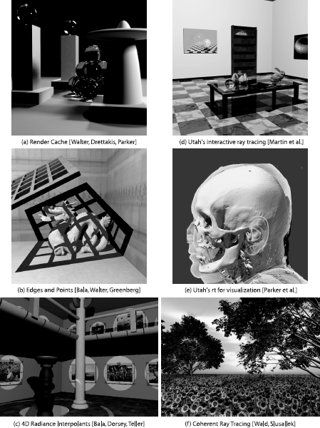
Images from interactive rendering systems. On the left are systems that use sparse sampling and interpolation: (a) render cache, (b) edges and points, and (c) 4D radiance interpolants. On the right are very fast ray tracers: (d) Utah’s interactive ray tracing, (e) Utah’s visualization of the visible female dataset, and (f) coherent ray tracing.
(See Plate XVIII.).
8.3.1 Sparse Sampling: Exploiting Coherence
Sparse sampling approaches try to decrease the huge gap in processor performance and rendering speeds by exploiting spatial and temporal coherence. These techniques sparsely sample shading values and cache these values. Images are then generated at interactive rates by interpolating these cached values when possible. Because they sparsely sample shading, and sometimes even visibility, they can substantially decrease the number of rays that must be traced per frame.
We briefly review several of these approaches. One major feature that differentiates between these approaches is how they cache and reuse samples. We categorize these algorithms as being image space, world space, or line space approaches based on how sampling and reconstruction is done.
Image Space
The render cache [211, 212] is an image-space algorithm that bridges the performance gap between processor performance and rendering speed by decoupling the display of images from the computation of shading. The display process runs synchronously and receives shading updates from a shading process that runs asynchronously. A fixed-size cache, the render cache, of shading samples (represented as three-dimensional points with color and position) is updated with the values returned by the shading process. As the user walks through a scene, the samples in the render cache are reprojected from frame to frame to the new viewpoint (similar to image-based reprojection techniques [16]). The algorithm uses heuristics to deal with disocclusions and other artifacts that arise from reprojection. The image at the new viewpoint is then reconstructed by interpolating samples in a 3 × 3 neighborhood of pixels. This interpolation filter smooths out artifacts and eliminates holes that might arise due to the inadequate availability of samples. A priority map is also computed at each frame to determine where new samples are needed. Aging samples are replaced by new samples.
The render cache produces images at interactive rates while sampling only a fraction of the pixels each frame. By decoupling the shader from the display process, the performance of the render cache depends on re-projection and interpolation and is essentially independent of the speed of the shader. This means the render cache can be used for interactive rendering with a slow (high-quality) renderer such as a path tracer. One disadvantage of the render cache is that the images could have visually objectionable artifacts because interpolation could blur sharp features in the image or reprojection could compute incorrect view-dependent effects.
The edge-and-point rendering system [9] addresses the problem of poor image quality in a sparse sampling and reconstruction algorithm by combining analytically computed discontinuities and sparse samples to reconstruct high-quality images at interactive rates. This approach introduces an efficient representation, called the edge and point image, to combine perceptually important discontinuities (edges), such as silhouettes and shadows, with sparse shading samples (points). The invariant maintained is that shading samples are never interpolated if they are separated by an edge. A render-cache–based approach is used to cache, reproject, and interpolate shading values while satisfying this edge-respecting invariant. The availability of discontinuity information further permits fast antialiasing. The edge-and-point renderer is able to produce high-quality, antialiased images at interactive rates using very low sampling densities at each frame. The edge-and-point image and the image filtering operations are well-matched for GPU acceleration [205], thus achieving greater performance.
World Space
The following techniques cache shading samples in object or world space and use the ubiquitous rasterization hardware to interpolate shading values to compute images in real time.
Tapestry [176] computes a three-dimensional world-space mesh of samples, where the samples are computed using a slow, high-quality renderer [107]. A Delaunay condition is maintained on the projection of the mesh relative to a viewpoint for robustness and image quality. A priority image is used to determine where more sampling is required. As the viewpoint changes, the mesh is updated with new samples while maintaining the De-launay condition.
Tole et al. [198] introduce the shading cache, an object-space hierarchical subdivision mesh where shading at vertices is also computed lazily. The mesh is progressively refined with shading values that, like the render cache and Tapestry, can be computed by a slow, high-quality, asynchronous shading process. The mesh is refined either to improve image quality or to handle dynamic objects. A priority image with flood filling is used to ensure that patches that require refining are given higher priority to be updated. A perceptual metric is used to age samples to account for view-dependent changes. This approach renders images in real time even with extremely slow asynchronous shaders (path tracers) and dynamic scenes.
Both these approaches use the graphics hardware to rasterize their meshes and interpolate the mesh samples to compute new images. In both techniques, visual artifacts arise while samples are accumulated and added to the meshes. However, these artifacts typically disappear as the meshes get progressively refined.
Line Space
Radiance is a function over the space of rays; this space is a five-dimensional space. However, in the absence of participating media and occluding objects, radiance does not vary along a ray. Thus, in free space, each radiance sample can be represented using four parameters; this space is called line space [57, 110]. We now discuss algorithms that cache samples in four-dimensional line space.
The radiance interpolants system [10], [8], [196] computes radiance samples lazily and caches these samples in four-dimensional line trees. Each leaf of the tree stores a radiance interpolant, a set of 16 radiance samples that can be interpolated to reconstruct radiance for any ray that lies in that leaf of the tree. One important contribution of this approach is the use of sophisticated interval-based techniques to bound the error that could arise by using interpolation to approximate shading. As the user walks around the scene, for each pixel in an image, the system uses a valid interpolant (if available) from the visible object’s line tree to approximate the pixel’s radiance. If no interpolant is available, the pixel is rendered using the ray tracer. This system achieves an order of magnitude speed-up in walk-throughs and successfully interpolates radiance for most pixels in each frame. The use of ray segment trees [7] (described below) further extends the radiance interpolant system to support dynamic scenes. While the error guarantees ensure that pixels are never incorrectly interpolated, since pixels are ray traced when a valid interpolant is not available, this system could be noninteractive for complex scenes.
The Holodeck [218] also caches samples in four-dimensional line space. These beams are stored on disk and recovered as needed to reconstruct images. Different reconstruction techniques are used based on Voronoi diagrams and Tapestry-like Delaunay triangulation of the samples.
8.3.2 Dynamic Scenes
One major challenge with caching shading values is dealing with dynamic scenes. When objects or lights move in a scene, the cached shading values could become invalid and must be updated accordingly. There are two reasons this update should be done incrementally. First, all these algorithms, to varying extents, assume the cached values accumulate over time. Recomputing all cached values from scratch would be too slow for interactive use. The second reason is that in typical interactive applications, the effect of an update (for example, an object being moved) can be quite localized.2 In such cases, updating all cached points unnecessarily is inefficient.
Some of the interactive rendering techniques, for example, the render cache and shading cache, age samples and eliminate outdated samples to ensure that all samples are recomputed from time to time. This ensures that images will eventually be correct once the moved objects are stationary for some number of frames. However, since these approaches do not explicitly find the effect of a scene change (for example, a moving shadow) and invalidate samples, they do not directly handle fully dynamic scenes.
Many techniques have been proposed to address this problem of invalidating samples in dynamic scenes. We briefly describe a few of them.
Drettakis and Sillion [39] introduce a four-dimensional line space hierarchy in the context of hierarchical radiosity to support dynamic scenes. When an object moves, this hierarchy of four-dimensional shafts is traversed at interactive rates to find the radiosity links that are affected by the object move.
Bala et al. [7] introduce a five-dimensional ray space hierarchy for updating radiance interpolants [8] in a ray-tracing context. A five-dimensional tree, called the ray segment tree, is used to rapidly find and invalidate all bundles of rays that are affected by an object movement. Their system starts to address updates in ray-traced applications but does not deal with full global illumination solutions. Selective photon tracing [38] uses the periodicity properties of quasi—Monte Carlo sampling sequences to rapidly identify and update the photons that are affected by changes in a scene. They progressively refine the global illumination solution to compute images in dynamic scenes.
All these techniques try to address the important problem of efficiently updating cached shading values in dynamic scenes. These approaches must satisfy two conflicting goals: correctness and efficiency. On the one hand, they must find all shading values that are affected by a change in the scene. On the other hand, they should avoid unnecessarily invalidating samples that remain accurate in spite of the change to the scene. While these approaches are promising, this is still an open area of research.
8.3.3 Fast Ray Tracing
The availability of increasingly fast processors and programmable GPUs is fueling research in systems for interactive ray tracing. These systems explore ray tracing as an alternative to hardware rendering because of ray tracing’s asymptotically superior performance in rendering complex scenes. When a ray tracer is supported by an acceleration structure (for example, octrees, kd-trees, or hierarchical bounding volumes), the cost of determining visibility for a single ray is typically logarithmic in scene complexity. In contrast, hardware, z-buffer algorithms render the entire scene each frame, achieving linear performance.3 Furthermore, ray tracers are extremely flexible and can support with full generality high-quality rendering effects. Thus, ray tracers are being considered as plausible alternatives for rendering complex scenes.
Parker et al. [137] implemented a highly optimized, parallel ray tracer to demonstrate the efficacy of ray tracing in interactive applications for complex scenes. They carefully tuned a shared-memory ray tracer on a 64-processor SGI Origin 2000 and exploited the fast synchronization capabilities and interconnect of the SGI Origin to achieve interactive performance. Load balancing was used to achieve linear speed-ups on the Origin. Their ray tracer was demonstrated rendering large scenes and visualizing extremely large data sets for scientific visualization, such as the visible female data set and crack propagation data sets.
Wald et al. [207, 208] have implemented interactive ray tracing in a cluster of PCs while paying careful attention to the performance of memory caches. Ray tracers, which traditionally do a depth-first traversal of rays, have poor memory access patterns. Their ray tracer exploits coherence by restructuring the order in which rays are traced to be a partial breadth-first evaluation.4 They avoid data replication over multiple processors by caching scene geometry on processors when needed. These performance optimizations give an order of magnitude speed-up and permit them to ray trace extremely large scenes at interactive rates. Subsequently, Reshetov et al. [152] introduce optimizations such as hierarchical beam tracing, to accelerate ray tracing performance in their multi level ray tracer.
8.3.4 Graphics Hardware and Precomputed Radiance Transfer
Modern graphics processing units (GPUs) are programmable parallel processors that provide flexibility by supporting vertex and pixel programma-bility. Apart from exploiting parallelism, GPUs also derive their power from their support for texturing, which requires very high memory bandwidth. In fact, the power and flexibility of GPUs has resulted in interest in GPUs as general computing systems. A branch of research called GPGPUs, for general purpose GPUs, treats GPUs as general stream processors and develops techniques to map general-purpose algorithms, for example, for sorting and linear algebra, on the GPU. On the graphics side, there has been increased interest in using the graphics hardware to integrate richer shading models and global illumination effects in rendered images. A description of these approaches is beyond the scope of this book, and the interested reader is referred to the books Real-Time Rendering [120] and Real-Time Shading [134] and the GPU Gems books [46, 144].
One deterrent to the practical application of global illumination in interactive applications is the significant time required to compute a full global illumination solution. While the advent of GPUs has decreased the cost of local pixel shading, the cost of determining visibility between two arbitrary points remains expensive. This is because this computation requires nonlocal access of data that is not cheap in the GPU model. Here, we discuss a few approaches that precompute visibility to achieve interactive rendering of high-quality illumination.
8.3.5 Ambient Occlusion
Ambient occlusion is a popular technique to “simulate” global effects in interactive applications. This approach precomputes and approximates the visibility between a point and the incoming hemisphere so that shading can be computed on the fly using this precomputed visibility term. While this technique is not accurate, it is fast and adds realism at a relatively low price. Ambient occlusion assumes rigid geometry and diffuse materials, though recent work attempts to relax the assumption of rigid geometry [20].
Ambient occlusion precomputes the visibility of the hemisphere at each point of the scene. This precomputation can be per-vertex or per-pixel, where the per-pixel information is encoded as textures. At each point (vertex or pixel), the algorithm samples the hemisphere to approximate visibility. This is where the assumption of view-independent diffuse materials comes into play. Using either uniform sampling or cosine-weighted sampling, the following integral is estimated as the ambient occlusion factor:
AO=1π∫ΩV(ω)(N⋅ω)dω. (8.14)
This precomputation is quite expensive. In the early days of the technique, several hardware-based approaches were developed to decrease the cost of this hemisphere sampling. However, with the availability of powerful ray tracers, ray tracing using Monte Carlo sampling is now the most popular and robust approach to compute the ambient occlusion.
Once the ambient occlusion values are computed, they are then used to render each point as follows. The simplest use is to modulate ambient lighting, just as its name suggests. In this case the precomputed ambient occlusion term is multiplied with a constant ambient term to achieve greater realism in the ambient shading term.
Ambient occlusion is also used, less accurately, to modulate more complex lighting environments, such as prefiltered environment maps. This is done by computing an additional value in the precomputation, the bent normal. The bent normal is the average unoccluded normal; i.e., it is the average normal of all unoccluded samples over the hemisphere. This bent normal approximates the main direction of illumination and is used when rendering the point instead of the surface normal. There are clear cases where the bent normal is inaccurate, but this approximation produces reasonable values for applications, such as movies and games, where accuracy is of less importance.
A generalization of ambient occlusion that is principled and accurate is discussed next: precomputed radiance transfer.
8.3.6 Precomputed Radiance Transfer
Precomputed radiance transfer (PRT) is a family of techniques that supports complex illumination effects by precomputing light transport and computing shading on the fly using the precomputed transport. This ability to support interactive performance with expensive shading has had a big impact on both research and practical applications such as games. We briefly introduce PRT concepts in this section and refer the reader to the original papers for details.
PRT uses precomputation to support expensive illumination effects such as interreflections, caustics, and subsurface scattering. However, to achieve interactive performance, some restrictions are imposed. PRT algorithms typically assume that the scene is static, and that lighting of the scene is from light sources that are infinitely far away, i.e., environment maps. In this section, we describe the basic PRT framework for diffuse materials lit by environment maps. We then describe the generalization of PRT concepts to support non-diffuse materials.
Diffuse PRT
The original PRT paper [177] illuminates diffuse and glossy objects lit by infinitely far away environment maps. For simplicity, let us first only consider direct illumination. The direct illumination at a point x, denoted as L0, is
L0(x→Θ)=∫ΩxLenv(x←Ψ)fr(x,Θ↔Ψ)cos(Ψ,Nx)dωΨ.
Since lighting is from a distant environment map, Lenv does not depend on position and only depends on direction. We further restrict ourselves to diffuse surfaces for now; thus, the BRDF is a constant and can be moved out of the integral:
L0(x)=ρπ∫ΩxLenυ(Ψ)V(x, Ψ) cos(Ψ, Nx)dωΨ.
The visibility V and cosine term are often combined together into a cosine-weighted visibility term.
The main insight of PRT is that this integral can be split into a pre-computed transfer function that includes the effects of self-shadowing and interreflections, and a runtime computation that efficiently combines the transfer function with the dynamically changing environment map.
To achieve this goal, PRT projects the lighting onto a set of basis functions over the sphere. The original formulation used spherical harmonics (SH). Thus, Lenv(Ψ) = ∑i liyi(Ψ), where the yi are the spherical harmonic basis functions and li are the lighting coefficients. Each li term is computed by projecting the environment map on the basis functions as follows: li = ∫Lenv (Ψ)yi (Ψ)dωΨ. Ramamoorthi [151] demonstrated that nine basis functions suffice to represent the appearance of diffuse surfaces lit by typical environment maps. For high-frequency shadowing, a potentially large set of basis functions are required. Since PRT aims at supporting shadows from relatively large area lights, the original PRT system used 25 basis functions.
Substituting the SH lighting coefficients, we get:
L0(x)=ρπ∫Ωx∑iliyi(Ψ)V(x,Ψ)cos(Ψ,Nx)dωΨ =ρπ∑ili∫Ωxyi(Ψ)V(x,Ψ)cos(Ψ,Nx)dωΨ =∑ilit0x,i,t0x,i=ρπ∫Ωxyi(Ψ)V(x,Ψ)cos(Ψ,Nx)dωΨ,
where the transfer function, represented as vector t, captures how an object casts shadows on itself (self-shadowing). The t0x, i are evaluated using Monte Carlo sampling.
The same derivation can be generalized to handle multiple reflections. We derive the generalization for the first bounce of illumination; the other bounces can straighforwardly be derived in a similar manner. We first simplify some of the notation: we denote the diffuse reflectivity at point x as ρx and point y as ρy, and the point y = r(x, Ψ) is the surface visible from x in direction Ψ. The first-bounce radiance L1 arriving at x through y is given as
L1(x)=∫Ωxρxπcos(Ψ,Nx)L0(y→−Ψ)dωΨL0(y→−Ψ)=∫Ωyρyπ cos(Ψ′,Ny)Lenv(Ψ′)dωΨ′=∑ilit0y,iL1(x)=∫Ωxρxπcos(Ψ,Nx)∑ilit0y,idωΨt1x,i=ρxπ∫Ωxt0y,icos(Ψ,Nx)dωΨ.
This approach can be generalized to more bounces. The corresponding terms for all bounces are added together to compute the total transfer function for each spherical harmonic basis function for the point x: tx, i=∑btbx, i. In these equations, the reflectivity has been folded into the transfer function for all bounces, direct and indirect. However, in fact, the reflectivity is often separated out for the direct bounce to permit denser BRDF sampling for directly visible surfaces.
A frame is rendered as follows. The environment map is projected into the spherical harmonic basis functions taking into account the object’s rotation with respect to the environment map. Rendering a vertex or pixel x then involves computing the dot product of the two vectors: the environment map coefficient vector l and the transfer function vector t for the point x. This dot product is easily supported on the GPU achieving interactive performance. Figure 8.18 shows results using diffuse PRT.
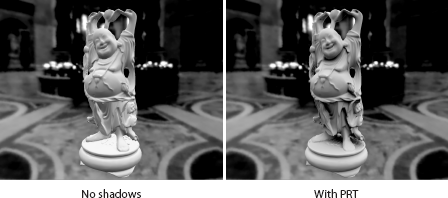
The Buddha model rendered with diffuse PRT using an environment map. Left: without shadows; right: with PRT.
(Image courtesy Peter-Pike Sloan and John Snyder.) (See Plate XXIV.)
The original PRT paper [177] introduced a powerful new technique for using precomputation to achieve interactive display of global illumination. Applications such as games for which interactive performance is crucial have adopted this basic approach. Some fairly major assumptions are made in the original formulation: static scenes, low-frequency environment maps, and diffuse and Phong-like materials. Subsequent research has tried to address these limitations. Kautz et al. [87] extends the SH transfer function vectors to handle arbitrary BRDFs; PCA clustering [178] further enables real-time performance.
All-Frequency PRT
High-frequency illumination effects, such as sharp shadows, cannot be represented with great fidelity using a small number of coefficients in the spherical harmonics basis functions. The next major set of innovations in PRT aim at supporting both all-frequency illumination effects and generalized BRDFs.
Ng et al. [129] introduce the use of wavelets for high-frequency illumination. Wavelet coefficients are selected on-the-fly to achieve a nonlinear approximation of high quality. This system demonstrates interactive performance for fixed viewing of nondiffuse scenes and arbitrary viewing of diffuse scenes. Figure 8.19 compares spherical harmonics with wavelets.
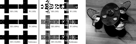
All-frequency effects. On the left, comparison of spherical harmonics (SH) and wavelets using nonlinear approximation (W) for the St. Peter’s Basilica environment map. On right, the triple product integral solution for a scene.
(Image courtesy Ren Ng and Ravi Ramamoorthi.) (See Plate XXIII.)
Liu et al. [113] and Wang et al. [215] approximate arbitrary, nondiffuse BRDFs by factoring them into components that are dependent on the viewing direction only and lighting direction only, respectively. Essentially, the 4D BRDF is split into two 2D functions that are separately approximated. Each separable function is represented using Haar wavelets, which are further clustered using PCA [113]. In this approach, the BRDF (and the cosine factor) are factored as: fr(x, Θ ↔ Ψ) cos(Ψ, Nx) = G(Θ)F(Ψ), where G and F are vector functions that depend entirely on the view direction Θ and the light direction Ψ, respectively. The final shading result is then GTMxL, where Mx is the linear transfer matrix at x, and L is the vector of lighting coefficients. It should be noted that BRDF separability is an approximation to the original BRDF, and it might not be valid and accurate for all BRDFs. Figure 8.20 shows results using this approach.
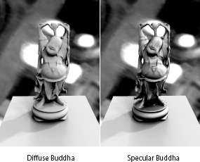
Diffuse and glossy Buddha rendered using PRT with separable BRDFs for high-frequency illumination.
(Image courtesy Peter-Pike Sloan and John Snyder.) (See Plate XXV.)
The triple product integral [130] takes a general approach to all-frequency lighting for direct illumination with nondiffuse materials. Radiance at x, where the BRDF term includes the cosine term and any rotation of the BRDF to align with the global coordinate frame, is:
L(x→Θ)=∫ΩxL(x←Ψ)fr(x,Θ↔Ψ)cos(Ψ,Nx)dωΨ=∫ΩxL(Ψ)f(Θ ↔ Ψ)V(x,Ψ)dωΨ.
The triple product integral approach uses this formulation of radiance as the product of three functions: lighting, material, and visibility. Each of these functions is projected into an orthonormal basis of functions: Lenv(Ψ) = ∑i liyi, f(Ψ) = ∑j fjyj, and V(Ψ) = ∑k vkyk. Ng et al. [130] developed efficient algorithms to use Haar wavelet basis functions for high-frequency effects.
The integral is then expressed using tripling coefficients, Cijk, as follows:
Cijk=∫yi(ω)yj(ω)yk(ω)dω.
The radiance at vertex or pixel x using the tripling coefficients is computed as
L=∑i∑j∑kCijklifjυk.
Figure 8.19 shows a scene rendered using triple product integrals encoded in Haar wavelets. The scene includes high-frequency shadows, glossy materials, and dynamic lighting from environment maps.
Summary of PRT
PRT remains an active area of research with several approaches that seek to generalize its applicability to support dynamics and a wide range of materials and illumination. Most PRT techniques assume the geometry is static: zonal harmonics are used to support deformable geometry in [180]; Kautz et al. [88] use hemispherical rasterization to recompute visibility for self-shadowing of dynamic objects; and Zhou et al. [229] precompute shadow fields for dynamic shadows from low-frequency illuminants. Support for subsurface scattering [178, 216] and bi-scale rendering [179] expands the range of materials and effects supported. Illumination from environment maps does not capture local lighting effects: Hasan et al. [66] extend fixed-viewpoint PRT for cinematic relighting, which requires support for arbitrary direct lighting, including high-frequency lighting shaders, with indirect illumination; Annen et al. [3] introduce spherical harmonic gradients to capture midrange illumination.
1The derivative of a function f(x) is, by definition, the limit of (f(x+Δx) — f(x))/Δx for Δx → 0.
2There are cases when this localized effect is not true, for example, when a light is moved.
3If hardware rendering is supported by sophisticated hierarchical data structures, its performance is logarithmic. However, these data structures require significant support from the application.
4In a noninteractive setting, Pharr et al. [146] also use restructuring of ray traversals to optimize memory access.