
Images computed with hierarchical Monte Carlo radiosity, with per-ray refinement (under 1 minute CPU time for up to 500,000 surface elements).
(See Figure 6.28.)
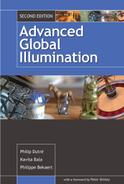
A car model rendering under real-world illumination, using a high dynamic range light probe (left images, photographs at various shutter times shown on top) and a histogram method.
(See Figure 6.14.)

Images rendered with a kernel density estimation method.
(Images courtesy of F. Drago and K. Myszkowski, Max-Planck-Institute for Informatics, Saarbrücken, Germany). (See Figure 6.15.)
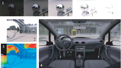
Images rendered with a kernel density estimation method.
(Images courtesy of B. Walter, Ph. Hubbard, P. Shirley, and D. Greenberg, Cornell Program of Computer Graphics). (See Figure 6.19.)

Left: Stochastic ray tracing; middle: light tracing; right: bidirectional ray tracing.
(Courtesy of F. Suykens-De Laet, Dept. of Computer Science, K. U. Leuven.) (See Figure 7.5.)

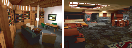
Bidirectional ray tracing. Note the extensive caustics, an effect difficult to achieve using stochastic ray tracing.
(Courtesy of F. Suykens-De Laet, Dept. of Computer Science, K. U. Leuven.) (See Figure 7.6.)


Irradiance caching example. Temple modeled by Veronica Sundstedt and Patrick Ledda.
(Courtesy of Greg Ward.) (See Figure 7.8.)
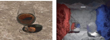
Examples of images produced using photon mapping. Figure (a) on the left shows caustics, while Figure (b) on the right shows a scene rendered with global illumination and displacement mapping.
(Courtesy of Henrik Wann Jensen.) (See Figure 7.11.)

These images show two views of the same scene, with only direct diffuse illumination besides specular reflections (left), and including indirect diffuse illumination (right), computed with a ray-tracing version of instant radiosity.
(Image courtesy of I. Wald, T. Kollig, C. Benthin, A. Keller, and Ph, Slusallek, Saarland University, Saarbrücken, and University of Kaiserslautern, Kaiserslautern, Germany.) (See Figure 7.13.)
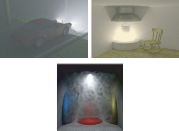
Some renderings of participating media: using bi-directional path tracing (top) and volume photon mapping (bottom).
(See Figure 8.6.)
![Figure showing two renderings of a translucent object. Left: using a standard BRDF model. Right: taking into account subsurface scattering with the dipole source model of [72].](http://imgdetail.ebookreading.net/software_development/6/9781439864951/9781439864951__advanced-global-illumination__9781439864951__image__347x002.png)
Two renderings of a translucent object. Left: using a standard BRDF model. Right: taking into account subsurface scattering with the dipole source model of [72].
(Image courtesy of T. Mertens, University of Limburg, Belgium.) (See Figure 8.9.)

Interference of light at a transparent thin film coating causes colorful reflections on these sunglasses.
(Image courtesy of Jay Gondek, Gary Meyer, and John Newman, University of Oregon.) (See Figure 8.12.)

The colorful reflections on this CD-ROM are caused by diffraction.
(Image courtesy of Jos Stam, Alias|Wavefront.) (See Figure 8.13.)

These images illustrate polarization of light reflected in the glass block on the left (Fresnel reflection). The same scene is shown, but with a different filter in front of the virtual camera: a horizontal polarization filter (left), vertical polarization filter (middle); and a 50% neutral gray (nonpolarizing) filter (right).
(Image courtesy of A. Wilkie, Vienna University of Technology, Austria.) (See Figure 8.14.)
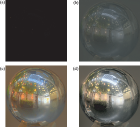
Various tone-mapping operators. (a) Linear scaling; (b) gamma scaling; (c) simple model of lightness sensitivity; (d) complex model for the human visual system.
(See Figure 8.15.)
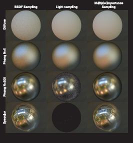
Combining BSDF sampling and light sampling with multiple importance sampling is always at least as good as BSDF sampling or light sampling alone.
(See Figure A.2.)

Images from interactive rendering systems. On the left are systems that use sparse sampling and interpolation: (a) render cache, (b) edges and points, and (c) 4D radiance interpolants. On the right are very fast ray tracers: (d) Utah’s interactive ray tracing, (e) Utah’s visualization of the visible female dataset, and (f) coherent ray tracing.
(See Figure 8.17.)

Photographing a light probe twice, 90 degrees apart. The camera positions are indicated in blue. Combining both photographs produces a well-sampled environment map without the camera being visible.
(Photographs courtesy of Vincent Masselus.) (See Figure 5.15.)

A simple scene with four point lights and the corresponding light tree. Each cut is a different partitioning of the lights into clusters. The cut shown in orange clusters lights three and four. The orange region in the rendered image (left) shows where the lightcut is a good approximation of the exact solution.
(Image courtesy Bruce Walter.) (See Figure 7.14.)

Scenes rendered using lightcuts. Tableau demonstrates glossy surfaces and HDR environment maps. The Kitchen scene includes area lights and the sun/sky model. Scalability graphs on the right show how cut size, and therefore performance, scales sublinearly with the number of lights. Big Screen includes two textured lights, the displays, each modeled with a point light source per pixel of the display. Grand Central Station includes 800 direct lights, sun/sky, and indirect illumination.
(Image courtesy Bruce Walter.) (See Figure 7.15.)


All-frequency effects. On the left, comparison of spherical harmonics (SH) and wavelets using nonlinear approximation (W) for the St. Peter’s Basilica environment map. On right, the triple product integral solution for a scene.
(Image courtesy Ren Ng and Ravi Ramamoorthi.) (See Figure 8.19.)

The Buddha model rendered with diffuse PRT using an environment map. Left: without shadows; right with PRT.
(Image courtesy Peter-Pike Sloan and John Snyder.) (See Figure 8.18.)
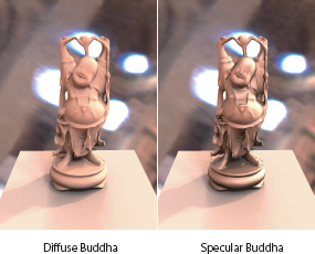
Diffuse and glossy Buddha rendered using PRT with separable BRDFs for high-frequency illumination.
(Image courtesy Peter-Pike Sloan and John Snyder.) (See Figure 8.20.)