Chapter 3

Monte Carlo Methods

This chapter introduces the concept of Monte Carlo integration and reviews some basic concepts in probability theory. We also present techniques to create better distributions of samples. More details on Monte Carlo methods can be found in Kalos and Whitlock [86], Hammersley and Hand-scomb [62], and Spanier and Gelbard [183]. References on quasi-Monte Carlo methods include Niederreiter [132].

3.1 Brief History

The term “Monte Carlo” was coined in the 1940s, at the advent of electronic computing, to describe mathematical techniques that use statistical sampling to simulate phenomena or evaluate values of functions. These techniques were originally devised to simulate neutron transport by scientists such as Stanislaw Ulam, John von Neumann, and Nicholas Metropolis, among others, who were working on the development of nuclear weapons. However, early examples of computations that can be defined as Monte Carlo exist, though without the use of computers to draw samples. One of the earliest documented examples of a Monte Carlo computation was done by Comte de Buffon in 1677. He conducted an experiment in which a needle of length L was thrown at random on a horizontal plane with lines drawn at a distance d apart (d > L). He repeated the experiment many times to estimate the probability P that the needle would intersect one of these lines. He also analytically evaluated P as

$P=\frac{2L}{\pi d}.$

Laplace later suggested that this technique of repeated experimentation could be used to compute an estimated value of π. Kalos and Whitlock [86] present early examples of Monte Carlo methods.

3.2 Why Are Monte Carlo Techniques Useful?

Consider a problem that must be solved, for example, computing the value of the integration of a function with respect to an appropriately defined measure over a domain. The Monte Carlo approach to solving this problem would be to define a random variable such that the expected value of that random variable would be the solution to the problem. Samples of this random variable are then drawn and averaged to compute an estimate of the expected value of the random variable. This estimated expected value is an approximation to the solution of the problem we originally wanted to solve.

One major strength of the Monte Carlo approach lies in its conceptual simplicity; once an appropriate random variable is found, the computation consists of sampling the random variable and averaging the estimates obtained from the sample. Another advantage of Monte Carlo techniques is that they can be applied to a wide range of problems. It is intuitive that Monte Carlo techniques would apply to problems that are stochastic in nature, for example, transport problems in nuclear physics. However, Monte Carlo techniques are applicable to an even wider range of problems, for example, problems that require the higher-dimensional integration of complicated functions. In fact, for these problems, Monte Carlo techniques are often the only feasible solution.

One disadvantage of Monte Carlo techniques is their relatively slow convergence rate of $\frac{1}{\sqrt{N}},$ where N is the number of samples (see Section 3.4). As a consequence, several variance reduction techniques have been developed in the field, discussed in this chapter. However, it should be noted that despite all these optimizations, Monte Carlo techniques still converge quite slowly and, therefore, are not used unless there are no viable alternatives. For example, even though Monte Carlo techniques are often illustrated using one-dimensional examples, they are not typically the most efficient solution technique for problems of this kind. But there are problems for which Monte Carlo methods are the only feasible solution technique: higher-dimensional integrals and integrals with nonsmooth integrands, among others.

3.3 Review of Probability Theory

In this section, we briefly review important concepts from probability theory. A Monte Carlo process is a sequence of random events. Often, a numerical outcome can be associated with each possible event. For example, when a fair die is thrown, the outcome could be any value from 1 to 6. A random variable describes the possible outcomes of an experiment.

3.3.1 Discrete Random Variables

When a random variable can take a finite number of possible values, it is called a discrete random variable. For a discrete random variable, a probability pi can be associated with any event with outcome xi.

A random variable xdie might be said to have a value of 1 to 6 associated with each of the possible outcomes of the throw of the die. The probability pi associated with each outcome for a fair die is 1/6.

Some properties of the probabilities pi are:

1. The probablity of an event lies between 0 and 1: 0 ≤ pi ≤ 1. If an outcome never occurs, its probability is 0; if an event always occurs, its probability is 1.

2. The probability that either of two events occurs is:

   $Pr \left(Even{t}_1\text{or}Even{t}_2\right)\le Pr \left(Even{t}_1\right)+Pr \left(Even{t}_2\right).$

   Two events are mutually exclusive if and only if the occurence of one of the events implies the other event cannot possibly occur. In the case of two such mutually exclusive events,

   $Pr \left(Even{t}_1\text{or}Even{t}_2\right)=Pr \left(Even{t}_1\right)+Pr \left(Even{t}_2\right).$

3. A set of all the possible events/outcomes of an experiment such that the events are mutually exclusive and collectively exhaustive satisfies the following normalization property: ${\displaystyle {\sum }_i{p}_i}=1$.

Expected Value

For a discrete random variable with n possible outcomes, the expected value, or mean, of the random variable is

$E\left(x\right)={\displaystyle \sum _{i=1}^n{p}_i}{x}_i.$

For the case of a fair die, the expected value of the die throws is

$\begin{array}{lll}\hfill E\left(x_{die}\right)& =\hfill & {\displaystyle \sum _{i=1}^6{p}_i}{x}_i\hfill \\ \hfill & =\hfill & {\displaystyle \sum _{i=1}^6\frac{1}{6}}{x}_i=\frac{1}{6}\left(1+2+3+4+5+6\right)\hfill \\ \hfill & =\hfill & \mathrm{3.5.}\hfill \end{array}$

Variance and Standard Deviation

The variance σ2 is a measure of the deviation of the outcomes from the expected value of the random variable. The variance is defined as the expected value of the square difference between the outcome of the experiment and its expected value. The standard deviation σ is the square root of the variance. The variance is expressed as

${\sigma }^2=E\left[{\left(x-E\left[x\right]\right)}^2\right]={{\displaystyle \sum _i\left(x_i-E\left[x\right]\right)}}^2{p}_i.$

Simple mathematical manipulation leads to the following equation:

${\sigma }^2=E\left[x^2\right]-{\left(E\left[x\right]\right)}^2={\displaystyle \sum _i{x}_i^2}{p}_i-{\left({\displaystyle \sum _i{x}_i{p}_i}\right)}^2.$

In the case of the fair die, the variance is

$\begin{array}{lll}\hfill {\sigma }_{die}^2& =\hfill & \frac{1}{6}[{(1–3.5)}^2+{(2–3.5)}^2+{(3–3.5)}^2+{(4–3.5)}^2\hfill \\ \hfill & \hfill & +{(5–3.5)}^2+{(6–3.5)}^2]\hfill \\ \hfill & =\hfill & \mathrm{2.91.}\hfill \end{array}$

Functions of Random Variables

Consider a function f(x), where x takes values xi with probabilities pi. Since x is a random variable, f(x) is also a random variable whose expected value or mean is defined as

$E\left[f\left(x\right)\right]={\displaystyle \sum _i{p}_{i}f\left(x_i\right)}.$

The variance of the function f(x) is defined similarly as

${\sigma }^2=E\left[{\left(f\left(x\right)-E\left[f\left(x\right)\right]\right)}^2\right].$

Example (Binomial Distribution)

Consider a random variable that has two possible mutually exclusive events with outcomes 1 and 0. These two outcomes occur with probability p and 1 – p, respectively. The expected value and variance of a random variable distributed according to this distribution are

$\begin{array}{lll}\hfill E\left[x\right]& =\hfill & 1·p+0·\left(1-p\right)=p;\hfill \\ \hfill {\sigma }^2& =\hfill & E\left[x^2\right]-E{\left[x\right]}^2=p-p^2=p(1-p).\hfill \end{array}$

Consider an experiment in which N random samples are drawn from the probability distribution above. Each sample can take a value of 0 or 1. The sum of these N samples is given as

$S={\displaystyle \sum _{i=1}^N{x}_i}.$

The probability that S = n, where n ≤ N, is the probability that n of the N samples take a value of 1, and N – n samples take a value of 0. This probability is

$Pr\left(S=n\right)=C_n^N{p}^n{\left(1-p\right)}^{N-n}.$

This distribution is called the binomial distribution. The binomial coefficient, CnN, counts the number of ways in which n of the N samples can take a value of 1: $C_n^N=\frac{N!}{\left(N-n\right)!n!}.$

The expected value of S is

$E\left[S\right]={\displaystyle \sum _{i=1}^{N}n{p}_i}={\displaystyle \sum n{C}_n^N}{p}^n{\left(1-p\right)}^{N-n}=Np.$

The variance is

${\sigma }^2=Np\left(1-p\right).$

This expected value and variance can be computed analytically by evaluating the expression:$a\frac{d}{da}{\left(a+b\right)}^N$, where a = p and b = (1 – p). Another possible way to compute the expected value and variance is to treat S as the sum of N random variables. Since these random variables are independent of each other, the expected value of S is the sum of the expected value of each variable as described in Section 3.4.1. Therefore, $E\left[S\right]={\displaystyle \sum E\left[x_i\right]}=Np.$

3.3.2 Continuous Random Variables

We have been discussing discrete-valued random variables; we will now extend our discussion to include continuous random variables.

Probability Distribution Function and Cumulative Distribution Function

For a real-valued (continuous) random variable x, a probability density function (PDF) p(x) is defined such that the probability that the variable takes a value x in the interval [x,x + dx] equals p(x)dx. A cumulative distribution function (CDF) provides a more intuitive definition of probabilities for continuous variables. The CDF for a random variable x is defined as follows:

$P\left(y\right)=Pr \left(x\le y\right)={\displaystyle {\int }_{-\infty }^{y}p\left(x\right)}dx.$

The CDF gives the probability with which an event occurs with an outcome whose value is less than or equal to the value y. Note that the CDF P(y) is a nondecreasing function and is non-negative over the domain of the random variable.

The PDF p(x) has the following properties:

$\begin{array}{l}\begin{array}{lll}\hfill \forall x:p\left(x\right)& \ge \hfill & 0;\hfill \\ {\displaystyle {\int }_{–\infty }^{\infty }p\left(x\right)dx}\hfill & =\hfill & 1;\hfill \end{array}\\ p\left(x\right)=\frac{dP\left(x\right)}{dx}.\end{array}$

Also,

$\begin{array}{lll}\hfill Pr \left(a\le x\le b\right)& =\hfill & Pr \left(x\le b\right)-Pr \left(x\le a\right)\hfill \\ \hfill & =\hfill & CDF\left(b\right)-CDF\left(a\right)={\displaystyle {\int }_a^{b}p\left(z\right)}dz.\hfill \end{array}$

Expected Value

Similar to the discrete-valued case, the expected value of a continuous random variable x is given as:

$E\left[x\right]={\displaystyle {\int }_{-\infty }^{\infty }xp\left(x\right)}dx.$

Now consider some function f(x), where p(x) is the probability distribution function of the random variable x. Since f(x) is also a random variable, its expected value is defined as follows:

$E\left[f\left(x\right)\right]={\displaystyle \int f\left(x\right)}p\left(x\right)dx.$

Variance and Standard Deviation

The variance σ2 for a continuous random variable is

${\sigma }^2=E\left[{\left(x-E\left[x\right]\right)}^2\right]={\displaystyle \int \left(x-E{\left[x\right]}^2\right)p\left(x\right)dx.}$

Simple mathematical manipulation leads to the following equation:

${\sigma }^2=E\left[x^2\right]-{\left(E\left[x\right]\right)}^2={\displaystyle \int x^{2}p\left(x\right)}dx-{\left({\displaystyle \int xp\left(x\right)dx}\right)}^2.$

Example (Uniform Probability Distribution)

For concreteness, we consider an example of one of the simplest probability distribution functions: the uniform probability distribution function. For a uniform probability distribution, the PDF is a constant over the entire domain, as depicted in Figure 3.1.

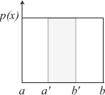
We know that ${\displaystyle {\int }_a^{b}p\left(x\right)dx=1}$. Therefore, the PDF pu for a uniform probability distribution function is

$p_u\left(x\right)=\frac{1}{b-a}.\left(3.1\right)$

The probability that x ∈ [a′, b′] is

$\begin{array}{lll}\hfill Pr \left(x\in \left[a^{\prime },b^{\prime }\right]\right)& =\hfill & {\displaystyle {\int }_{a^{\prime }}^{b^{\prime }}\frac{1}{b-a}}dx\hfill \\ \hfill & =\hfill & \frac{b^{\prime }-a^{\prime }}{b-a};\hfill \\ \hfill Pr \left(x\le y\right)=CDF\left(y\right)& =\hfill & {\displaystyle {\int }_{-\infty }^y\frac{1}{b-a}}dx\hfill \\ \hfill & =\hfill & \frac{y-a}{b-a}.\hfill \end{array}$

For the special case where a = 0, b = 1:

$Pr \left(x\le y\right)=CDF\left(y\right)=y.$

3.3.3 Conditional and Marginal Probabilities

Consider a pair of random variables x and y. For discrete random variables, pij specifies the probability that x takes a value of xi and y takes a value of yi. Similarly, a joint probability distribution function p(x, y) is defined for continuous random variables.

The marginal density function of x is defined as

$p\left(x\right)={\displaystyle \int p\left(x,y\right)}dy.$

Similarly, for a discrete random variable, $p_i={\displaystyle {\sum }_j{p}_{ij}}$.

The conditional density function p(y|x) is the probability of y given some x:

$p\left(y|x\right)=\frac{p\left(x,y\right)}{p\left(x\right)}=\frac{p\left(x,y\right)}{{\displaystyle \int p\left(x,y\right)dy}}.$

The conditional expectation of a random function g(x, y) is computed as

$E\left[g|x\right]={\displaystyle \int g\left(x,y\right)}p\left(y|x\right)dy=\frac{{\displaystyle \int g\left(x,y\right)p\left(x,y\right)dy}}{{\displaystyle \int p\left(x,y\right)dy}}.$

These definitions are useful for multidimensional Monte Carlo computations.

3.4 Monte Carlo Integration

We now describe how Monte Carlo techniques can be used for the integration of arbitrary functions. Let us assume we have some function f(x) defined over the domain x ∈ [a, b]. We would like to evaluate the integral

$I={\displaystyle {\int }_a^{b}f\left(x\right)}dx.\left(3.2\right)$

We will first illustrate the idea of Monte Carlo integration in the context of one-dimensional integration and then extend these ideas to higher-dimensional integration. However, it should be mentioned that several effective deterministic techniques exist for one-dimensional integration, and Monte Carlo is typically not used in this domain.

3.4.1 Weighted Sum of Random Variables

Consider a function G that is the weighted sum of N random variables g(x1), ...g(xN), where each of the xi has the same probability distribution function p(x). The xi variables are called independent identically distributed (IID) variables. Let gi(x) denote the function g(xi):

$G={\displaystyle \sum _{j=1}^N{w}_j{g}_j.}$

The following linearity property can easily be proved:

$E\left[G\left(x\right)\right]={\displaystyle \sum _j{w}_j}E\left[g_j\left(x\right)\right].$

Now consider the case where the weights wj are the same and all add to 1. Therefore, when N functions are added together, wj = 1/N:

$\begin{array}{ccc}\hfill G\left(x\right)& =\hfill & {\displaystyle \sum _{j=1}^N{w}_j}{g}_j\left(x\right)\hfill \\ \hfill & =\hfill & {\displaystyle \sum _{j=1}^N\frac{1}{N}}{g}_j\left(x\right)\hfill \\ \hfill & =\hfill & \frac{1}{N}{\displaystyle \sum _{j=1}^N{g}_j\left(x\right).}\hfill \end{array}$

The expected value of G(x) is

$\begin{array}{ccc}\hfill E\left[G\left(x\right)\right]& =\hfill & {\displaystyle \sum _j{w}_j}E\left[g_j\left(x\right)\right]\hfill \\ \hfill & =\hfill & \frac{1}{N}{\displaystyle \sum _{j=1}^{N}E\left[g_j\left(x\right)\right]}\hfill \\ \hfill & =\hfill & \frac{1}{N}{\displaystyle \sum _{j=1}^{N}E\left[g\left(x\right)\right]}\hfill \\ \hfill & =\hfill & \frac{1}{N}NE\left[g\left(x\right)\right]\hfill \\ \hfill & =\hfill & E\left[g\left(x\right)\right].\hfill \end{array}$

Thus, the expected value of G is the same as the expected value of g(x). Therefore, G can be used to estimate the expected value of g(x). G is called an estimator of the expected value of the function g(x).

The variance of G is

${\sigma }^2\left[G\left(x\right)\right]={\sigma }^2\left[{\displaystyle \sum _{i=1}^N\frac{g_i\left(x\right)}{N}}\right].$

Variance, in general, satisfies the following equation:

${\sigma }^2\left[x+y\right]={\sigma }^2\left[x\right]+{\sigma }^2\left[y\right]+2Cov\left[x,y\right],$

with the covariance Cov [x, y] given as

$Cov\left[x,y\right]=E\left[xy\right]-E\left[x\right].E\left[y\right].$

In the case of independent random variables, the covariance is 0, and the following linearity property for variance does hold:

${\sigma }^2\left[x+y\right]={\sigma }^2\left[x\right]+{\sigma }^2\left[y\right].$

This result generalizes to the linear combination of several variables.

The following property holds for any constant a:

${\sigma }^2\left[ax\right]=a^2{\sigma }^2\left[x\right].$

Using the fact that the xi in G are independent identically distributed variables, we get the following variance for G:

${\sigma }^2\left[G\left(x\right)\right]={\displaystyle \sum _{i=1}^N{\sigma }^2}\left[\frac{g_i\left(x\right)}{N}\right].$

Therefore,

$\begin{array}{ccc}\hfill {\sigma }^2\left[G\left(x\right)\right]& =\hfill & {\displaystyle \sum _{i=1}^N\frac{{\sigma }^2\left[g\left(x\right)\right]}{N^2}}\hfill \\ \hfill & =\hfill & N\frac{{\sigma }^2\left[g\left(x\right)\right]}{N^2}\hfill \\ \hfill & =\hfill & \frac{{\sigma }^2\left[g\left(x\right)\right]}{N}.\hfill \end{array}$

Thus, as N increases, the variance of G decreases with N, making G an increasingly good estimator of E[g(x)]. The standard deviation σ decreases as $\sqrt{N}$.

3.4.2 Estimator

The Monte Carlo approach to computing the integral is to consider N samples to estimate the value of the integral. The samples are selected randomly over the domain of the integral with probability distribution function p(x). The estimator is denoted as 〈I〉 and is

$\langle I\rangle =\frac{1}{N}{\displaystyle \sum _{i=1}^N\frac{f\left(x_i\right)}{p\left(x_i\right)}}.$

In Section 3.6.1, we explain why samples are computed from a probability distrubtion p(x) as opposed to uniform sampling of the domain of the integration. Let us for now accept that p(x) is used for sampling.

Using the properties described in Section 3.4.1, the expected value of this estimator is computed as follows:

$\begin{array}{lll}\hfill E\left[\langle I\rangle \right]& =\hfill & E\left[\frac{1}{N}{\displaystyle \sum _{i=1}^N\frac{f\left(x_i\right)}{p\left(x_i\right)}}\right]\hfill \\ \hfill & =\hfill & \frac{1}{N}{\displaystyle \sum _{i=1}^{N}E\left[\frac{f\left(x_i\right)}{p\left(x_i\right)}\right]}\hfill \\ \hfill & =\hfill & \frac{1}{N}N{\displaystyle \int \frac{f\left(x\right)}{p\left(x\right)}}p\left(x\right)dx\hfill \\ \hfill & =\hfill & {\displaystyle \int f\left(x\right)}dx\hfill \\ \hfill & =\hfill & I.\hfill \end{array}$

Also, from Section 3.4.1, we know that the variance of this estimator is

${\sigma }^2=\frac{1}{N}{{\displaystyle \int \left(\frac{f\left(x\right)}{p\left(x\right)}-I\right)}}^{2}p\left(x\right)dx.$

Thus, as N increases, the variance decreases linearly with N. The error in the estimator is proportional to the standard deviation σ; the standard deviation decreases as $\sqrt{N.}$ This is a classic result of Monte Carlo methods. In fact one problem with Monte Carlo is the slow convergence of the estimator to the right solution; four times more samples are required to decrease the error of the Monte Carlo computation by half.

Example (Monte Carlo Summation)

A discrete sum $S={\displaystyle {\sum }_{i=1}^n{s}_i}$ can be computed using the estimator 〈S〉 = nx, where x takes the value of each term of the sum si with equal probability 1/n. We can see that the expected value of the estimator is S. Using the estimator, the following algorithm can be used to estimate the sum S: Randomly select a term si where each term has the same chance of being selected 1/n. An estimate of the sum is the product of the value of the selected term times the number of terms: nsi.

Since computing sums is clearly a very efficient computation in modern computers, it might appear that the above algorithm is not very useful. However, in cases where the sum consists of complex terms that are time-consuming to compute, this technique of sampling sums is useful. We show how this technique is used in Chapter 6.

Example (Simple MC Integration)

Let us show how Monte Carlo integration works for the following simple integral:

$I={\displaystyle {\int }_0^{1}5x^4}dx.$

Using analytical integration, we know that the value of this integral is 1. Assuming samples are computed from a uniform probability distribution

(i.e., p(x) = 1 over the domain [0,1)), our estimator would be

$\langle I\rangle =\frac{1}{N}{\displaystyle \sum _{i=1}^{N}5x_i^4}.$

A possible evaluation of this integral using Monte Carlo techniques is shown in Figure 3.2.

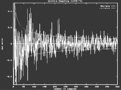
The variance of this function can be analytically computed as follows:

${\sigma }_{est}^2=\frac{1}{N}{{\displaystyle {\int }_0^1\left(5x^4-1\right)}}^{2}dx=\frac{16}{9N}.$

As N increases, we get an increasingly better approximation of the integral.

3.4.3 Bias

When the expected value of the estimator is exactly the value of the integral I (as is the case for the estimator described above), the estimator is said to be unbiased. An estimator that does not satisfy this property is said to be biased; the difference between the expected value of the estimator and the actual value of the integral is called bias: B[〈I〉] = E[〈I〉] – I. The total error on the estimate is typically represented as the sum of the standard deviation and the bias. The notion of bias is important in characterizing different approaches to solving a problem using Monte Carlo integration.

A biased estimator is called consistent if the bias vanishes as the number of samples increases; i.e., if limN → ∞ B[〈I〉] = 0. Sometimes, it is useful to use biased estimators if they result in a lower variance that compensates for the bias introduced. However, we must analyze both variance and bias for these estimators, making the analysis more complicated than for unbiased estimators.

3.4.4 Accuracy

Two theorems explain how the error of the Monte Carlo estimator reduces as the number of samples increases. Remember that these error bounds are probabilistic in nature.

The first theorem is Chebyshev’s Inequality, which states that the probability that a sample deviates from the solution by a value greater than $\sqrt{\frac{{\sigma }^2}{\delta }},$ where δ is an arbitrary positive number, is smaller than δ. This inequality is expressed mathematically as

$Pr \left[|\langle I\rangle -E\left[I\right]|\ge \sqrt{\frac{{\sigma }_I^2}{\delta }}\right]\le \delta ,$

where δ is a positive number. Assuming an estimator that averages N samples and has a well-defined variance, the variance of the estimator is

${\sigma }_I^2=\frac{1}{N}{\sigma }_{primary}^2.$

Therefore, if $\delta =\frac{1}{10000},$

$Pr \left[|\langle I\rangle -E\left[I\right]|\ge \frac{100{\sigma }_{primary}}{\sqrt{N}}\right]\le \frac{1}{10000}.$

Thus, by increasing N, the probability that 〈I〉 ≈ E[I] is very large.

The Central Limit Theorem gives an even stronger statement about the accuracy of the estimator. As N → ∞, the Central Limit Theorem states that the values of the estimator have a normal distribution. Therefore, as N → ∞, the computed estimate lies in a narrower region around the expected value of the integral with higher probability. Thus, the computed estimate is within one standard deviation of the integral 68.3% of the time, and within three standard deviations of the integral 99.7% of the time. As N gets larger, the standard deviations, which vary as $\frac{1}{\sqrt{N}},$ get smaller and the estimator estimates the integral more accurately with high probability.

However, the Central Limit Theorem only applies when N is large enough; how large N should be is not clear. Most Monte Carlo techniques assume that N is large enough; though care should be taken when small values of N are used.

3.4.5 Estimating the Variance

The variance of a Monte Carlo computation can be estimated using the same N samples that are used to compute the original estimator. The variance for the Monte Carlo estimator is

$\begin{array}{lll}\hfill {\sigma }^2& =\hfill & \frac{1}{N}{{\displaystyle \int \left(\frac{f\left(x\right)}{p\left(x\right)}-I\right)}}^{2}p\left(x\right)dx\hfill \\ \hfill & =\hfill & \frac{1}{N}{{\displaystyle \int \left(\frac{f\left(x\right)}{p\left(x\right)}\right)}}^{2}p\left(x\right)dx-I^2\hfill \\ \hfill & =\hfill & \frac{1}{N}{\displaystyle \int \frac{f{\left(x\right)}^2}{p\left(x\right)}dx-I^2.}\hfill \end{array}$

The variance itself can be estimated by its own estimator σ2est [86]:

${\sigma }_{est}^2\approx \frac{\frac{1}{N}{{\displaystyle {\sum }_{i=1}^N\left(\frac{f\left(x_i\right)}{p\left(x_i\right)}\right)}}^2-{\left(\frac{1}{N}{\displaystyle {\sum }_{i=1}^N\frac{f\left(x_i\right)}{p\left(x_i\right)}}\right)}^2}{N-1}.$

3.4.6 Deterministic Quadrature versus Monte Carlo

As a point of comparison, note that a deterministic quadrature rule to compute a one-dimensional integral could be to compute the sum of the area of regions (perhaps uniformly spaced) over the domain (see Figure 3.3). Effectively, one approximation of the integral I would be

$I\approx {\displaystyle \sum _{i=1}^N{w}_{i}f\left(x_i\right)}={\displaystyle \sum _{i=1}^N\frac{f\left(x_i\right)\left(b-a\right)}{N}}.$

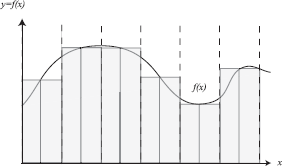
The trapezoidal rule and other rules [149] are typical techniques used for one-dimensional integration. Extending these deterministic quadrature rules to a d-dimensional integral would require Nd samples.

3.4.7 Multidimensional Monte Carlo Integration

The Monte Carlo integration technique described above can be extended to multiple dimensions in a straightforward manner as follows:

$\begin{array}{lll}\hfill I& =\hfill & {\displaystyle \int {\displaystyle \int f\left(x,y\right)dxdy}}\hfill \\ \hfill \langle I\rangle & =\hfill & \frac{1}{N}{\displaystyle \sum _{i=1}^N\frac{f\left(x_i,y_i\right)}{p\left(x_i,y_i\right)}.}\hfill \end{array}$

One of the main strengths of Monte Carlo integration is that it can be extended seamlessly to multiple dimensions. Unlike deterministic quadrature techniques, which would require Nd samples for a d-dimensional integration, Monte Carlo techniques permit an arbitrary choice of N.

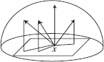
Example (Integration over a Hemisphere)

Let us consider a simple example of Monte Carlo integration over a hemisphere. The particular problem we want to solve is to estimate the irra-diance at a point by integrating the contribution of light sources in the scene.

Let us consider a light source L. To compute the irradiance due to the light source, we must evaluate the following integral:

$\begin{array}{lll}\hfill I& =\hfill & {\displaystyle \int L_{source}}\cos \theta d{\omega }_{\text{Θ}}\hfill \\ \hfill & =\hfill & {\displaystyle {\int }_0^{2\pi }{\displaystyle {\int }_0^{\frac{\pi }{2}}{L}_{source}}}\cos \theta \sin \theta d\theta d\varphi .\hfill \end{array}$

The estimator for irradiance is:

$\langle I\rangle =\frac{1}{N}{\displaystyle \sum _{i=1}^N\frac{L_{source}\left({\text{Θ}}_i\right)\cos \theta \sin \theta }{p\left({\text{Θ}}_i\right)}}.$

We can choose our samples from the following probability distribution:

$p\left({\text{Θ}}_i\right)=\frac{\cos \theta \sin \theta }{\pi }.$

The estimator for irradiance is then given as

$\langle I\rangle =\frac{\pi }{N}{\displaystyle \sum _{i=1}^N{L}_{source}}\left({\text{Θ}}_i\right).$

3.4.8 Summary of Monte Carlo

In summary a Monte Carlo estimator for an integral $I={\displaystyle \int f\left(x\right)dx}$ is

$\langle I\rangle =\frac{1}{N}{\displaystyle \sum _{i=1}^N\frac{f\left(x_i\right)}{p\left(x_i\right)}}.$

The variance of this estimator is

${\sigma }^2=\frac{1}{N}{{\displaystyle \int \left(\frac{f\left(x\right)}{p\left(x\right)}-I\right)}}^{2}p\left(x\right)dx.$

Monte Carlo integration is a powerful, general technique that can handle arbitrary functions. A Monte Carlo computation consists of the following steps:

• Sampling according to a probability distribution function.
• Evaluation of the function at that sample.
• Averaging these appropriately weighted sampled values.

The user only needs to understand how to do the above three steps to be able to use Monte Carlo techniques.

3.5 Sampling Random Variables

We have discussed how the Monte Carlo technique must compute samples from a probability distribution p(x). Therefore, we want to find samples such that the distribution of the samples matches p(x). We now describe different techniques to achieve this sampling.

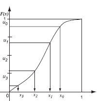
3.5.1 Inverse Cumulative Distribution Function

To intuitively illustrate the inverse cumulative distribution function (CDF) technique, we first describe how to sample according to a PDF for a discrete PDF. We then extend this technique to a continuous PDF.

Discrete Random Variables

Given a set of probabilities pi, we want to pick xi with probability pi. We compute the discrete cumulative probability distribution (CDF) corresponding to the pi as follows: $F_i={\displaystyle {\sum }_{j=1}^i{p}_i}.$ Now, the selection of samples is done as follows. Compute a sample u that is uniformly distributed over the domain [0,1). Output k that satisfies the property:

$\begin{array}{lll}\hfill F_{k-1}& \le \hfill & u \text{<} F_k;\hfill \\ \hfill {\displaystyle \sum _{j=1}^{k-1}{p}_j}& \le \hfill & u \text{<} {\displaystyle \sum _{j=1}^k{p}_j};\hfill \\ \hfill {\displaystyle \sum _{j=1}^{k-1}{p}_j}& \le \hfill & u \text{<} F_{k-1}+p_k.\hfill \end{array}$

We know from Equation 3.1 for a uniform PDF, F(a ≤ u < b) = (b – a). Clearly, the probability that the value of u lies between Fk – 1 and Fk is Fk – Fk – 1 = pk. But this is the probability that k is selected. Therefore, k is selected with probability pk, which is exactly what we want.

The F values can be computed in O(n) time; the look-up of the appropriate value to output can be done in O(log2(n)) time per sample by doing a binary search on the precomputed F table.

Continuous Random Variables

The approach above can be extended to continuous random variables. A sample can be generated according to a given distribution p(x) by applying the inverse cumulative distribution function of p(x) to a uniformly generated random variable u over the interval [0, 1). The resulting sample is F–1(u). This technique is illustrated in Figure 3.5.

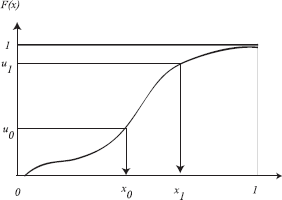
Pick u uniformly from [0,1)

Output y = F–1(u)

The resulting samples have the distribution of p(x) as can be proved below:

$F\left(y\right)={\displaystyle {\int }_{-\infty }^{y}p\left(x\right)}dx.$

We want to prove that

$Pr \left[y\le Y\right]={\displaystyle {\int }_{-\infty }^{Y}p\left(x\right)}dx.$

Consider the new samples we compute. For every uniform variable u, we compute the sample as y = F–1 (u). From Equation 3.1, we know that

$Pr \left[u\le X\right]=X.$

Therefore,

$\begin{array}{lll}\hfill Pr \left[F^{-1}\left(u\right)\le F^{-1}\left(X\right)\right]& =\hfill & X\hfill \\ \hfill \text{if} X& =\hfill & F\left(Y\right)\hfill \\ \hfill Pr \left[y\le Y\right]& =\hfill & F\left(Y\right)={\displaystyle {\int }_{-\infty }^{Y}p\left(x\right)}dx.\hfill \end{array}$

Note that the fact that the cumulative probability distribution function is a monotonically nondecreasing function is important in the proof above. Also note that this method of sampling requires the ability to compute and analytically invert the cumulative probability distribution.

Example (Cosine Lobe)

A cosine weighting factor arises in the rendering equation; therefore, it is often useful to sample the hemisphere to compute radiance using a cosine PDF. We show how the hemisphere can be sampled such that the samples are weighted by the cosine term.

The PDF is

$p\left(\theta ,\varphi \right)=\frac{\cos \theta }{\pi }.$

Its CDF is computed as described above:

$\begin{array}{lll}\hfill F& =\hfill & \frac{1}{\pi }{\displaystyle \int \cos \theta d\omega ;}\hfill \\ \hfill F\left(\theta ,\varphi \right)& =\hfill & \frac{1}{\pi }{\displaystyle {\int }_0^{\varphi }{\displaystyle {\int }_0^{\theta }\cos {\theta }^{\prime }\sin {\theta }^{\prime }d{\theta }^{\prime }d{\varphi }^{\prime }}}\hfill \\ \hfill & =\hfill & \frac{1}{\pi }{\displaystyle {\int }_0^{\varphi }d{\varphi }^{\prime }{\displaystyle {\int }_0^{\theta }\cos {\theta }^{\prime }\sin {\theta }^{\prime }d{\theta }^{\prime }}}\hfill \\ \hfill & =\hfill & \frac{\varphi }{\pi }\left(-{\cos }^2{\theta }^{\prime }/2\right){|}_0^{\theta }\hfill \\ \hfill & =\hfill & \frac{\varphi }{2\pi }\left(1-{\cos }^2\theta \right).\hfill \end{array}$

The CDF, with respect to ϕ and θ functions, is separable:

$\begin{array}{lll}\hfill F_{\varphi }& =\hfill & \frac{\varphi }{2\pi };\hfill \\ \hfill F_{\theta }& =\hfill & 1-{\cos }^2\theta .\hfill \end{array}$

Therefore, assuming we compute two uniformly distributed samples u1 and u2:

${\varphi }_i=2\pi u_1$

and

${\theta }_i={\cos }^{-1}\sqrt{u_{2,}}$

where 1 — u is replaced by u2 since the uniform random variables lie in the domain [0,1). These ϕi and θi values are distributed according to the cosine PDF.

3.5.2 Rejection Sampling

It is often not possible to derive an analytical formula for the inverse of the cumulative distribution function. Rejection sampling is an alternative that could be used and was one of the primary techniques used in the field in the past. In rejection sampling, samples are tentatively proposed and tested to determine acceptance or rejection of the sample. This method raises the dimension of the function being sampled by one and then uniformly samples the bounding box that includes the entire PDF. This sampling technique yields samples with the appropriate distribution.

Let us see how this works for a one-dimensional PDF whose maximum value over the domain [a, b] to be sampled is M. Rejection sampling raises the dimension of the function by one and creates a two-dimensional function over [a, b] × [0, M]. This function is then sampled uniformly to compute samples (x,y). Rejection sampling rejects all samples (x,y) such that p(x) < y. All other samples are accepted. The distribution of the accepted samples is exactly the PDF p(x) we want to sample.

Compute sample xi uniformly from the domain of x

Compute sample ui uniformly from [0, 1)

if $u_i\le \frac{p\left(x_i\right)}{M}$ then return xi

else reject sample

One criticism of rejection sampling is that rejecting these samples (those that lie in the unshaded area of Figure 3.6) could be inefficient. The efficiency of this technique is proportional to the probabilty of accepting a proposed sample. This probability is proportional to the ratio of the area under the function to the area of the box. If this ratio is small, a lot of samples are rejected.

3.5.3 Look-Up Table

Another alternative for sampling PDFs is to use a look-up table. This approach approximates the PDF to be sampled using piecewise linear approximations. This technique is not commonly used though it is very useful when the sampled PDF is obtained from measured data.

3.6 Variance Reduction

Monte Carlo integration techniques can be roughly subdivided into two categories: those that have no information about the function to be integrated (sometimes called blind Monte Carlo), and those that do have some kind of information (sometimes called informed Monte Carlo). Intuitively one expects that informed Monte Carlo methods are able to produce more accurate results as compared to blind Monte Carlo methods. The Monte Carlo integration algorithm outlined in Section 3.4 would be a blind Monte Carlo method if the samples were generated uniformly over the domain of integration without any information about the function being integrated.

Designing efficient estimators is a major area of research in Monte Carlo literature. A variety of techniques that reduce variance have been developed. We discuss some of these techniques in this section: importance sampling, stratified sampling, multiple importance sampling, the use of control variates, and quasi-Monte Carlo.

3.6.1 Importance Sampling

Importance sampling is a technique that uses a nonuniform probability distribution function to generate samples. The variance of the computation can be reduced by choosing the probability distribution wisely based on information about the function to be integrated.

Given a PDF p(x) defined over the integration domain D, and samples xi generated according to the PDF, the value of the integral I can be estimated by generating N sample points and computing the weighted mean:

$\langle I\rangle =\frac{1}{N}{\displaystyle \sum _{i=1}^N\frac{f\left(x_i\right)}{p\left(x_i\right)}}.$

As proven earlier, the expected value of this estimator is I; therefore, the estimator is unbiased. To determine if the variance of this estimator is better that an estimator using uniform sampling, we estimate the variance as described in Section 3.4.5. Clearly, the choice of p(x) affects the value of the variance. The difficulty of importance sampling is to choose a p(x) such that the variance is minimized. In fact, a perfect estimator would have the variance be zero.

The optimal p(x) for the perfect estimator can be found by minimizing the equation of the variance using variational techniques and Lagrange multipliers as below. We have to find a scalar λ for which the following expression L, a function of p(x), reaches a minimum,

$L\left(p\right)={{\displaystyle {\int }_D\left(\frac{f\left(x\right)}{p\left(x\right)}\right)}}^{2}p\left(x\right)dx+\text{λ}{\displaystyle {\int }_{D}p\left(x\right)}dx,$

where the only boundary condition is that the integral of p(x) over the integration domain equals 1, i.e.,

${\displaystyle {\int }_{D}p\left(x\right)}dx=1.$

This kind of minimization problem can be solved using the Euler-Lagrange differential equation:

$L\left(p\right)={\displaystyle {\int }_D\left(\frac{f{\left(x\right)}^2}{p\left(x\right)}+\text{λ}p\left(x\right)\right)}dx.$

To minimize the function, we differentiate L(p) with respect to p(x) and solve for the value of p(x) that makes this quantity zero:

$\begin{array}{lll}\hfill 0& =\hfill & \frac{\partial }{\partial p}\left(\frac{f{\left(x\right)}^2}{p\left(x\right)}+\text{λ}p\left(x\right)\right)\hfill \\ \hfill 0& =\hfill & -\frac{f^2\left(x\right)}{p^2\left(x\right)}+\text{λ}\hfill \\ \hfill p\left(x\right)& =\hfill & \frac{1}{\sqrt{\text{λ}}}\left|f\left(x\right)\right|.\hfill \end{array}$

The constant $\frac{1}{\sqrt{\text{λ}}}$ is a scaling factor, such that p(x) can fulfill the boundary condition. The optimal p(x) is then given by:

$p\left(x\right)=\frac{\left|f\left(x\right)\right|}{{\displaystyle {\int }_{D}f\left(x\right)dx}}.$

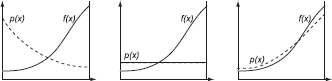
If we use this p(x), the variance will be exactly 0 (assuming f(x) does not change sign). However, this optimal p(x) requires us to know the value of the integral ∫D f(x)dx. But this is exactly the integral we want to compute to begin with! Clearly, finding the optimal p(x) is not possible. However, importance sampling can still be a major tool in decreasing variance in Monte Carlo techniques. Intuitively, a good importance sampling function matches the “shape” of the original function as closely as possible. Figure 3.7 shows three different probability functions, each of which will produce an unbiased estimator. However, the variance of the estimator on the left-hand side will be larger than the variance of the estimator shown on the right-hand side.

3.6.2 Stratified Sampling

One problem with the sampling techniques that we have described is that samples can be badly distributed over the domain of integration resulting in a poor approximation of the integral. This clumping of samples can happen irrespective of the PDF used, because the PDF only tells us something about the expected number of samples in parts of the domain. Increasing the number of samples collected will eventually address this problem of uneven sample distribution. However, other techniques have been developed to avoid the clumping of samples: one such technique is stratified sampling.

The basic idea in stratified sampling is to split the integration domain into m disjoint subdomains (also called strata) and evaluate the integral in each of the subdomains separately with one or more samples. More precisely,

$\begin{array}{lll}\hfill {\displaystyle {\int }_0^{1}f(x)dx}& =\hfill & {\displaystyle {\int }_0^{{\alpha }_1}f(x)dx+{\displaystyle {\int }_{{\alpha }_1}^{{\alpha }_2}f(x)dx+...}}\hfill \\ \hfill & \hfill & +{\displaystyle {\int }_{{\alpha }_{m–2}}^{{\alpha }_{m–1}}f(x)dx+}{\displaystyle {\int }_{{\alpha }_{m–1}}^{1}f(x)dx.}\hfill \end{array}$

Stratified sampling often leads to a smaller variance as compared to a blind Monte Carlo integration method. The variance of a stratified sampling method, where each stratum receives a number of samples nj, which are in turn distributed uniformly over their respective intervals, is equal to

${\sigma }^2={\displaystyle \sum _{j=1}^m\frac{{\alpha }_j–{\alpha }_{j–1}}{n_j}}{\displaystyle {\int }_{{\alpha }_{j–1}}^{{\alpha }_j}f{\left(x\right)}^{2}dx–}{\displaystyle \sum _{j=1}^m\frac{1}{n_j}{\left({\displaystyle {\int }_{{\alpha }_{j–1}}^{{\alpha }_j}f\left(x\right)dx}\right)}^2.}$

If all the strata are of equal size (αj — αj – 1 = 1/m), and each stratum contains one uniformly generated sample (nj = 1;N = m), the above equation can be simplified to:

$\begin{array}{lll}\hfill {\sigma }^2& =\hfill & {\displaystyle \sum _{j=1}^m\frac{1}{N}}{\displaystyle {\int }_{{\alpha }_{j–1}}^{{\alpha }_j}f{\left(x\right)}^{2}dx–}{\displaystyle \sum _{j=1}^m{\left({\displaystyle {\int }_{{\alpha }_{j–1}}^{{\alpha }_j}f\left(x\right)dx}\right)}^2}\hfill \\ \hfill & =\hfill & \frac{1}{N}{\displaystyle {\int }_0^{1}f{\left(x\right)}^{2}dx–}{\displaystyle \sum _{j=1}^N{\left({\displaystyle {\int }_{{\alpha }_{j–1}}^{{\alpha }_j}f\left(x\right)dx}\right)}^2}.\hfill \end{array}$

This expression indicates that the variance obtained using stratified sampling is always smaller than the variance obtained by a pure Monte Carlo sampling scheme. As a consequence, there is no advantage in generating more than one sample within a single stratum, since a simple equal subdivision of the stratum such that each sample is attributed to a single stratum always yields a better result.

This does not mean that the above sampling scheme always gives us the smallest possible variance; this is because we did not take into account the size of the strata relative to each other and the number of samples per stratum. It is not an easy problem to determine how these degrees of freedom can be chosen optimally, such that the final variance is the smallest possible. It can be proven that the optimal number of samples in one subdomain is proportional to the variance of the function values relative to the average function value in that subdomain. Applied to the principle of one sample per stratum, this implies that the size of the strata should be chosen such that the function variance is equal in all strata. Such a sampling strategy assumes prior knowledge of the function in question, which is often not available. However, such a sampling strategy might be used in an adaptive sampling algorithm.

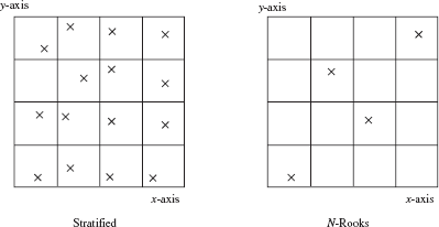
Stratified sampling works well when the number of samples required is known in advance and the dimensionality of the problem is relatively low (typically less than 20). The number of strata required does not scale well with an increase in the number of dimensions. For a d-dimensional function, the number of samples required is Nd, which can be prohibitive for large values of d. Several techniques can be used to control the increase in the number of samples with the increase in dimensions. The N-rooks algorithm keeps the number of samples fixed (irrespective of dimensionality). Quasi– Monte Carlo sampling uses nonrandom samples to avoid clumping. Both of these techniques are described below.

3.6.3 N-Rooks or Latin Hypercube Algorithm

As mentioned, one major disadvantage of stratified sampling arises when it is used for higher-dimensional sampling. Consider, for example, a two-dimensional function; stratification of both dimensions would require N2 strata with one sample per stratum. The N-rooks algorithm addresses this by distributing N samples evenly among the strata. Each dimension is still subdivided into N subintervals. However, only N samples are needed; these samples are distributed such that one sample lies in each subinterval.

This distribution is achieved by computing permutations of 1..N (let us call them q0, q1, ...), and letting the ith d-dimensional sample be:

$\left(\frac{q_0\left(i\right)–u_0}{N},\frac{q_1\left(i\right)–u_1}{N},...,\frac{q_{d–1}\left(i\right)–u_{d–1}}{N}\right).$

In two dimensions, this means that no row or column has more than one sample. An example distribution is shown in Figure 3.8.

3.6.4 Combining Stratified Sampling and Importance Sampling

Stratified sampling can easily be integrated with importance sampling: the samples computed from a uniform probability distribution can be stratified, and then these stratified samples are transformed using the inverse cumulative distribution function. This strategy (shown in Figure 3.9) avoids the clumping of samples, while at the same time distributing the samples according to the appropriate probability distribution function.

Example (Stratified Sampling of Discrete Sums)

The following example illustrates how stratification can be combined with importance sampling. Stratification of the following sum, $S={\displaystyle {\sum }_{i=1}^n{a}_i}$, with probabilities pi, is done using the following code [124]:

Compute a uniformly distributed random number u in [0,1)

Initialize: Nsum = 0, P = 0

for i = 1 to n

   P += pi

   Ni = [P n + u] — Nsum

   Sample the ith term of the sum Ni times

   Nsum += Ni

A single random number u is computed using the above algorithm. The ith term of the sum is sampled Ni times, where Ni is computed as above.

3.6.5 Combining Estimators of Different Distributions

We have explained that importance sampling is an effective technique often used to decrease variance. The function f could consist of the product of several different functions: importance sampling according to any one of these PDFs could be used. Each of these techniques could be effective (i.e., have a low variance) depending on the parameters of the function. It is useful to combine these different sampling techniques so as to obtain robust solutions that have low variance over a wide range of parameter settings. For example, the rendering equation consists of the BRDF, the geometry term, the incoming radiance, etc. Each one of these different terms could be used for importance sampling. However, depending on the material properties or the distribution of objects in a scene, one of these techniques could be more effective than the other.

Using Variance

Consider combining two estimators, 〈I1〉 and 〈I2〉, to compute an integral I. Clearly, any linear combination w1〈I1〉 + w2〈I2〉 with constant weights w1 + w2 = 1 will also be an estimator for S. The variance of the linear combination however depends on the weights,

${\sigma }^2\left[w_1\langle I_1\rangle +w_2\langle I_2\rangle \right]=w_1^2{\sigma }^2\left[\langle I_1\rangle \right]+w_2^2{\sigma }^2\left[\langle I_2\rangle \right]+2w_1{w}_2\text{Cov}\left[\langle I_1\rangle \langle I_2\rangle \right],$

where Cov[〈I1〉 〈I2〉] denotes the covariance of the two estimators:

$\text{Cov}\left[\langle I_1\rangle \langle I_2\rangle \right]=E\left[\langle I_1\rangle .\langle I_2\rangle \right]-E\left[\langle I_1\rangle \right].E\left[\langle I_2\rangle \right].$

If 〈I1〉 and 〈I2〉 are independent, the covariance is zero. Minimization of the variance expression above allows us to fix the optimal combination weights:

$\frac{w_1}{w_2}=\frac{{\sigma }^2\left[\langle I_2\rangle \right]-\text{Cov}\left[\langle I_1\rangle ,\langle I_2\rangle \right]}{{\sigma }^2\left[\langle I_1\rangle \right]-\text{Cov}\left[\langle I_1\rangle ,\langle I_2\rangle \right]}.$

For independent estimators, the weights should be inversely proportional to the variance. In practice, the weights can be calculated in two different ways:

1. Using analytical expressions for the variance of the involved estimators (such as presented in this text).
2. Using a posteriori estimates for the variances based on the samples in an experiment themselves [86]. By doing so, a slight bias is introduced. As the number of samples is increased, the bias vanishes: the combination is asymptotically unbiased or consistent.

Multiple Importance Sampling

Veach [204] described a robust strategy, called multiple importance sampling, to combine different estimators using potentially different weights for each individual sample, even for samples from the same estimator. Thus, samples from one estimator could have different weights assigned to them, unlike the approach above where the weight depends only on the variance. The balance heuristic is used to determine the weights that combine these samples from different PDFs provided the weights sum to 1. The balance heuristic results in an unbiased estimator that provably has variance that differs from the variance of the “optimal estimator” by an additive error term. For complex problems, this strategy is simple and robust.

Let the sample computed from technique i with PDF pi be denoted Xij, where j = 1, ..,ni. The estimator using the balance heuristic is

$F=\frac{1}{N}{\displaystyle \sum _{i=1}^n{\displaystyle \sum _{j=i}^{n_i}\frac{f\left(X_{i,j}\right)}{{\displaystyle {\sum }_k{c}_k{p}_k\left(X_{i,j}\right)}}}},$

where $N={\displaystyle {\sum }_i{n}_i}$ is the total number of samples and ck = nk/N is the fraction of samples from technique k.

The balance heuristic is computed as follows:

$N={\displaystyle {\sum }_{i=1}^n{n}_i}$

for i = 1 to n

   for j = 1 to ni

     X = Sample(pi)

     $d={\displaystyle {\sum }_{k=1}^n\left(n_k/N\right) p_k\left(X\right)}$

     F = F + f(X)/d

return F/N

3.6.6 Control Variates

Another technique to reduce variance uses control variates. Variance could be reduced by computing a function g that can be integrated analytically and subtracted from the original function to be integrated.

$\begin{array}{lll}\hfill I& =\hfill & {\displaystyle \int f\left(x\right)}dx\hfill \\ \hfill & =\hfill & {\displaystyle \int g\left(x\right)}dx+{\displaystyle \int f\left(x\right)}-g\left(x\right)dx.\hfill \end{array}$

Since the integral of the function ∫ g(x)dx has been computed analytically the original integral is estimated by computing an estimator for ∫ f(x) — g(x)dx.

If f(x) — g(x) is almost constant, this technique is very effective at decreasing variance. If f/g is nearly constant, g should be used for importance sampling [86].

3.6.7 Quasi-Monte Carlo

Quasi-Monte Carlo techniques decrease the effects of clumping in samples by eliminating randomness completely. Samples are deterministically distributed as uniformly as possible. Quasi-Monte Carlo techniques try to minimize clumping with respect to a measure called the discrepancy.

The most commonly used measure of discrepancy is the star discrepancy measure described below. To understand how quasi–Monte Carlo techniques distribute samples, we consider a set of points P. Consider each possible axis-aligned box with one corner at the origin. Given a box of size Bsize, the ideal distribution of points would have NBsize points. The star discrepancy measure computes how much the point distribution P deviates from this ideal situation,

$D_N^{*}\left(P\right)={\mathit{sup}}_B|\frac{NumPoints\left(P\cap B\right)}{N}-B_{size}|,$

where NumPoints(P ∩ B) are the number of points from the set P that lie in box B.

The star discrepancy is significant because it is closely related to the error bounds for quasi-Monte Carlo integration. The Koksma-Hlawka inequality [132] states that the difference between the estimator and the integral to be computed satisifes the condition:

$|\frac{1}{N}{\displaystyle \sum _{k=1}^{N}f\left(x_k\right)}-{\displaystyle {\int }_0^{1}f\left(x\right)}dx|\le V_{HK}\left(f\left(x\right)\right)D^{*},$

where the VHK term is the variation in the function f(x) in the sense of Hardy and Krause. Intuitively, VHK measures how fast the function can change. If a function has bounded and continuous mixed derivatives, then its variation is finite.

The important point to take from this inequality is that the error in the MC estimate is directly proportional to the discrepancy of the sample set. Therefore, much effort has been expended in designing sequences that have low discrepancy; these sequences are called low-discrepancy sequences (LDS).

There are several low-discrepancy sequences that are used in quasi-Monte Carlo techniques: Hammersley Halton, Sobol, and Niederreiter, among others. We describe a few of these sequences here.

Halton sequences are based on the radical inverse function and are computed as follows. Consider a number i which is expressed in base b with the terms aj :

$i={\displaystyle \sum _{j=0}^{\infty }{a}_j\left(i\right)}{b}^j.$

The radical inverse function Φ is obtained by reflecting the digits about the decimal point:

${\text{Φ}}_b\left(i\right)={\displaystyle \sum _{j=0}^{\infty }{a}_j\left(i\right)}{b}^{-j-1}.$

Examples of the radical inverse function for numbers 1 through 6 in base 2 (b = 2) are shown in Table 3.1. To compare the radical inverse function for different bases, consider the number 11 in base 2: i = 10112. The radical inverse function Φ2(11) = .11012 = 1/2 + 1/4 + 1/16 = 0.8125. In base 3, Φ3(11) = .2013 = 2/3 + 1/27 = 0.7037.

The discrepancy of the radical inverse sequence is O((log N)/N) for any base b. To obtain a d-dimensional low-discrepancy sequence, a different radical-inverse sequence is used in each dimension. Therefore, the ith point in the sequence is given as

$x_i=\left({\text{Φ}}_{b_1}\left(i\right),{\text{Φ}}_{b_2}\left(i\right),{\text{Φ}}_{b_3}\left(i\right),\mathrm{....},{\text{Φ}}_{b_d}\left(i\right)\right),$

where the bases bj are relatively prime.

The Halton sequence for d dimensions sets the bi terms to be the first d prime numbers; i.e., 2, 3, 5, 7, ..., and so on. The Halton sequence has a discrepancy of O((log N)d/N). Intuitively, the reason the Halton sequence is uniform can be explained as follows: This sequence produces all binary strings of length m before producing strings of length m + 1. All intervals of size 2–m will be visited before a new point is put in the same interval.

When the number of samples required N is known ahead of time, the Hammersley sequence could be used for a slightly better discrepancy. The ith point of the Hammersley sequence is

$x_i=\left(\frac{i}{N},{\text{Φ}}_{b_1}\left(i\right),{\text{Φ}}_{b_2}\left(i\right),{\text{Φ}}_{b_3}\left(i\right),\mathrm{...},{\text{Φ}}_{b_{d-1}}\left(i\right)\right).$

This sequence is regular in the first dimension; the remaining dimensions use the first (d – 1) prime numbers. The discrepancy of the Hammersley point set is O((log N)d – 1/N).

Other sequences, such as the Niederreiter, are also useful for Monte Carlo computations [19].

Why Quasi–Monte Carlo?

The error bound for low-discrepancy sequences when applied to MC integration is O((log N)d/N) or O((log N)d – 1/N) for large N and dimension d. This bound could have a substantial potential benefit compared to the $1/\sqrt{N}$ error bounds for pure Monte Carlo techniques. Low-discrepancy sequences work best for low dimensions (about 10-20); at higher dimensions, their performance is similar to pseudorandom sampling. However, as compared to pseudorandom sampling, low-discrepancy sequences are highly correlated; e.g., the difference between successive samples in the van der Corput sequence (a base-2 Halton sequence) is 0.5 half of the time; Table 3.1 shows this.

The upshot is that low-discrepancy sampling gives up randomness in return for uniformity in the sample distribution.

3.7 Summary

In this chapter, we have described Monte Carlo integration techniques and discussed their accuracy and convergence rates. We have also presented variance reduction techniques such as importance sampling, stratified sampling, the use of control variates, multiple importance sampling, and quasi– Monte Carlo sampling. More details on MC methods can be found in Ka-los and Whitlock [86], Hammersley and Handscomb [62], and Spanier and Gelbard [183]. References on quasi–Monte Carlo methods include Nieder-reiter [132].

3.8 Exercises

1. Write a program to compute the integral of a one-dimensional function using Monte Carlo integration. Plot the absolute error versus the number of samples used. This requires that you know the an alytic answer to the integral, so use well-known functions such as polynomials.

   Experiment with various optimization techniques such as stratified sampling and importance sampling. Draw conclusions about how the error due to the Monte Carlo integration is dependent on the sampling scheme used.

2. Using the algorithm designed above, try to compute the integral for sine functions with increasing frequencies. How is the error influenced by the various frequencies over the same integration domain?
3. Write a program to compute the integral of a two-dimensional function using Monte Carlo integration. This is very similar to the first exercise, but using two-dimensional functions poses some additional problems. Experiment with stratified sampling versus N-rooks sampling, as well as with importance sampling. Again, plot absolute error versus number of samples used.

4. Implement an algorithm to generate uniformly distributed points over a triangle in the 2D-plane. Start with a simple triangle first (connecting points (0,0), (1, 0) and (0, 1)), then try to generalize to a random triangle in the 2D plane.

   How can such an algorithm be used to generate points on a triangle in 3D space?

5. Pick an interesting geometric solid in 3D: a sphere, cone, cylinder, etc. Design and implement an algorithm to generate uniformly distributed points on the surface of these solids. Visualize your results to make sure the points are indeed distributed uniformly.