2. Financial Review and Pro Forma Analysis
Market View
In 2007, Microsoft purchased aQuantive, an online advertising company. At the time, the acquisition was the software giant’s largest ever. Microsoft paid $6.3 billion in cash, an 85 percent premium over aQuantive’s share price, to jump-start its online advertising business and challenge Google, which had recently purchased DoubleClick, one of aQuantive’s key competitors. The online advertising market was worth $25 billion in 2007, and it had experienced a growth of 30 percent year-on-year.
Microsoft viewed the acquisition of aQuantive as an opportunity to capture a significant share of this growing market and boost its online revenue and profit. Five years later, Microsoft announced that it was taking an accounting charge of $6.2 billion, largely tied to the acquisition of aQuantive. Although the write-off did not affect Microsoft’s financial health, it was a clear indication that the company had overpaid for aQuantive. According to the press release, “While the Online Services Division business [primarily aQuantive] has been improving, the company’s expectations for future growth and profitability are lower than previous estimates.” Microsoft had to admit that it had overvalued, and consequently overpaid, for aQuantive.
Analysts hoped that Microsoft had learned the lesson. A few months earlier, it had paid $8.5 billion to purchase Skype Technologies, the Internet calling service. Skype had turned out to be a bad acquisition for its previous owner, eBay. In 2005, eBay outbid Google and Yahoo! to acquire loss-making Skype for $2.6 billion. It later spent another $530 million in payouts to Skype’s founders. In 2007, eBay wrote off $1.43 billion, recognizing that it had dramatically overpaid for Skype. Unable to make the acquisition work, eBay sold a 65 percent stake to private equity investors in 2009. Two years later, these private equity investors brokered a deal with Microsoft, giving eBay the opportunity to sell its remaining stake in Skype. Although eBay did not disclose the net effect of its investment in Skype, it was estimated that the company made a few hundred million dollars—a good outcome for a bad acquisition.
Microsoft and eBay are among many companies that overpaid for their acquisitions and subsequently had to write off a significant portion of the purchase price. One of the key reasons companies overpay is that they overvalue the target—that is, they overestimate the target’s revenue and profit and end up paying more than the target is worth.
Why do more than half of mergers and acquisitions (M&As) erode shareholder value? And why do many transactions fail to earn a rate of return at least equivalent to the cost of the capital necessary to finance them? The answer to both questions is often the same: overestimation of the target’s value. The process of valuing a company presents innumerable opportunities for biases and errors, and analysts and corporate executives frequently err on the positive side when assessing the value of a company. Research in behavioral finance has shown that people are subject to cognitive errors and emotional biases. One such emotional bias is overconfidence. An analyst might be overly optimistic about a company’s growth prospects or might have excessive confidence in his or her forecasts, resulting in an inflated value for the target. In addition, executives’ overconfidence may affect their judgment and lead them to overpay. The predisposition to overpay when making acquisitions has been referred to as the winner’s curse, in that winning a bidding war for a target could actually mean losing and destroying shareholder value.
This chapter begins our exploration of the process of valuing a company. We assume that a target has been identified and that the acquisition appears desirable from a strategic perspective. One of the first questions that arises when starting the valuation process is, “What does the future hold for the target?” Answering this question requires reviewing the recent past and developing forecasts about the future. In this chapter, we formalize the historical review of a target by means of financial review, and we develop forecasts by means of pro forma analysis.
Specifically, this chapter addresses the following key questions:
• How should the historical financial review of a target be organized?
• Which financial ratios should be calculated?
• How can forecasts be developed?
• How can the sensitivity of the forecasts to key assumptions be evaluated?
1 Financial Review
Financial review is the process of analyzing, evaluating, and describing the financial history of a company. It is a key element of the process of due diligence that precedes any acquisition offer. Financial review serves four key functions when an acquisition candidate is being valued. First, it provides the necessary information for an acquirer to confirm that a target is a financially appropriate and desirable acquisition. Second, it helps the analyst gain an understanding of the fundamental business model of the target and determine the key revenue and cost drivers of the company. Third, it identifies the target’s financial strengths and weaknesses, and hence the factors that will enhance or reduce the benefits associated with the acquisition. Finally, it provides a set of benchmark relationships that the analyst needs to build a realistic set of forecasts. As discussed shortly, the common-size financial statements and ratios developed as part of the historic financial review often provide the key percentage estimates used to build forecast earnings and cash flows.
The techniques of financial review are many and varied, and we limit our consideration to the techniques most relevant to the valuation process: ratio analysis and cash flow analysis. Ratio analysis is the process of investigating the relationship among various balance sheet, income statement, and cash flow statement accounts. Analysts use ratios to investigate these relationships across multiple time periods through what is commonly called trend analysis, or among various alternative targets in what is traditionally labeled cross-section analysis. In addition to comparing ratios over time for a given target or between alternative targets, it is often advisable for an analyst to compare a target’s ratios to industry-wide indices. Financial data vendors such as Moody’s Analytics, Morningstar, Thomson Reuters, Standard & Poor’s, and Value Line, among others, provide industry data that allow a company’s performance to be compared against the average performance of companies within a given industry. This type of comparison enables the analyst to assess the relative performance of a target candidate against a set of comparable companies.
Cash flow analysis refers to the process of identifying the various sources and uses of cash flows of a target. This analysis addresses the following questions:
• Is the target generating a positive cash flow from its operations?
• How has the target been using its available cash resources—to replace property, plant, and equipment; to pay dividends; to retire debt; or to repurchase shares?
• How has the target been financing its capital expenditures—from operations, debt or equity issuances, or asset liquidation?
• Is the target likely to need a cash infusion after the acquisition?
Because cash is the primary investment attribute for investors, the analysis of cash flows is particularly significant in the process of financial review.
1.1. Ratio Analysis
Analysts have always faced the problem of deciding how to organize the financial review of a company. It is commonly acknowledged that the four key areas of interest are profitability, asset turnover, financial leverage, and shareholders’ return. One framework that has been successfully implemented to link profitability and asset turnover is the DuPont model, named after the company in which it was developed.
1.1.1. The DuPont Model
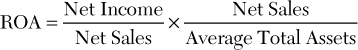
The DuPont model features a company’s return on assets (ROA) as the quintessential measure of firm and managerial performance:
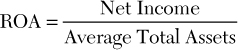
Note that the denominator of the ROA is an average. When analysts calculate a ratio that includes both an income statement account and a balance sheet account, they often average the beginning-of-period and the end-of-period balance sheet values. In doing so, they increase the comparability of the balance sheet account with the income statement account because both accounts reflect an entire period (such as one year or one quarter). For example, if the company experienced a significant increase or decrease in the value of its total assets throughout the period, it would distort the ROA to divide a company’s net income (which is accumulated throughout the period) by the ending total assets (which is a snapshot of the last day of the period); the ROA would end up being biased by the expansion or contraction in total assets throughout the period. By considering both the beginning-of-period and end-of-period values, the average total assets offers a better reflection of the level of assets that was in place throughout the period to generate the profit for the period.
One advantage of the DuPont model, shown in Exhibit 2.1, is that it highlights the important interplay between profitability and asset turnover—namely, that a company’s ROA can be positively affected by the following:
• Increasing the net profit margin on each sale transaction
• Increasing the volume of sales transactions, given its existing asset base (total asset turnover)
• Some combination of increasing the net profit margin and increasing the total asset turnover

In essence, the DuPont model focuses on the income statement and the left (asset) side of the balance sheet. It helps analysts evaluate a company’s earnings and investment in assets and thus assess the company’s business risk. Unfortunately, the DuPont model ignores the important issue of how a company has financed its investment in assets—does it use debt, and if it does, what is the amount of borrowings relative to the amount of equity? By ignoring the right (liabilities and equity) side of the balance sheet, the DuPont model does not assess the company’s financial risk.
1.1.2. The ROE Model
To overcome this limitation, many analysts have turned to an extension of the DuPont model, known as the return on shareholders’ equity model, or ROE model. The ROE model is broader in scope than the DuPont model because it considers a company’s financing decisions as well as its business (operating and investing) decisions. The strength of the ROE model is not only that it integrates both business and financial decisions, but also that it relies on the widely held notion that the primary goal of management is to maximize shareholder value. The cornerstone of the ROE model is the return on equity, a shareholder-based ratio of performance:

The ROE is the rate of return generated by a company for its owners—that is, the voting (or common) shareholders. It can be decomposed into two key components:1

Or:
ROE = ROA × Financial Leverage
The first component of a company’s ROE is its ROA, the cornerstone of the DuPont model. The second component reflects the company’s financial leverage; it tells us whether the company uses debt in its capital structure and, if it does, the extent to which the company finances its assets with borrowed money. The decomposition of the ROE clearly shows that a company’s performance depends on two factors: (1) How profitably the company uses its assets, and (2) whether management has successfully leveraged the owners’ investment in the company. The more profitably a company uses its assets, the greater the return is to its owners. A second way to maximize shareholders’ return is to use debt. If a company can generate a return on its borrowed assets that exceeds its cost of borrowing, the company can enhance its ROE by leveraging the owners’ investment. However, it is important to observe that financial leverage is a double-edged sword: Debt enhances a company’s ROE only as long as the return generated on the borrowed assets exceeds the cost of borrowing. If a company uses debt to invest in assets that return less than the cost of borrowing, financial leverage reduces a company’s ROE and destroys shareholder value.
The ROE can be further decomposed by examining the individual factors that contribute to the ROA and financial leverage. As Exhibit 2.1 shows, the ROA depends on two factors: (1) the relative profitability of each sale that a company generates (its net profit margin) and (2) the volume of sales generated, given the company’s existing asset base (its total asset turnover). Specifically:2
Or:
ROA = Net Profit Margin × Total Asset Turnover
Returning to the ROE model:
ROE = Net Profit Margin × Total Asset Turnover × Financial Leverage
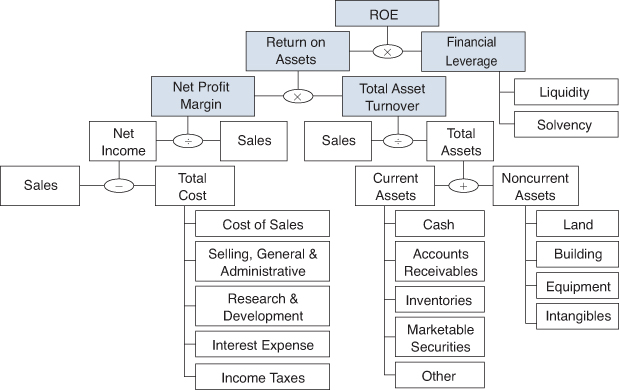
This equation reveals the three primary drivers of shareholders’ return are: (1) the relative profitability of each sale that a company generates, (2) the volume of sales generated, given the company’s existing asset base, and (3) the extent to which the company has been able to successfully leverage its owners’ investment. Exhibit 2.2 shows how the ROE model builds on and extends the DuPont model.
We illustrate the ROE model with the financial data for Mattel, one of the world’s largest toy manufacturers headquartered in the United States. Appendix 2A shows Mattel’s financial statements for the period 2008–2011. Exhibit 2.3 presents Mattel’s ratios for the four-year period.3
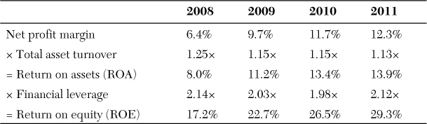
Between 2008 and 2011, Mattel’s ROE increased from 17.2 percent to 29.3 percent. This increase was driven by an increase in its ROA, from 8.0 percent in 2008 to 13.9 percent in 2011. The decomposition of the ROA between the net profit margin and the total asset turnover shows that the increase in the ROA resulted from an improvement in the net profit margin. Mattel generated 6.4 cents of profit per dollar of sales revenue in 2008, whereas the profit per dollar of sales revenue nearly doubled, to 12.3 cents, in 2011. However, the total asset turnover deteriorated during the four-year period. Mattel generated $1.25 of sales per dollar of assets in 2008, whereas a dollar of assets yielded only $1.13 of sales in 2011. Because the net profit margin improvement was stronger than the total asset turnover deterioration, the joint effect of these two ratios on the ROA was positive.
Exhibit 2.3 reveals that Mattel uses debt in its capital structure and that the financial leverage had a positive effect on the company’s performance: The ROE is higher than the ROA, indicating that the use of debt financing enhanced the shareholders’ return. Mattel reduced its financial leverage from 2.14 times in 2008 to 1.98 times in 2010, but increased its borrowings between 2010 and 2011, returning to a level of financial leverage in 2011 similar to that in 2008.
1.2. Decomposition Analysis
Just as it is possible to decompose the ROE into its three key drivers of net profit margin, asset turnover, and financial leverage, it is possible to decompose each of these three key drivers into their subcomponents. Decomposition analysis is the process of segmenting a component of the ROE into its subcomponents and, in doing so, enabling the analyst to begin the process of identifying the specific causes of change in each of the key ROE drivers.
1.2.1. Decomposing Net Profit Margin
A company’s net profit margin indicates the relative profitability of its operations. Decomposing the net profit margin enables the analyst to identify which component(s) of operations were responsible for generating a change in profitability.
The most effective way to decompose a company’s net profit margin into its subcomponents is with common-size income statements. In common-size financial statements, all amounts are expressed as a percentage of some base financial statement account. For common-size income statements, all amounts are expressed as a percentage of net sales; for common-size balance sheets, all amounts are expressed as a percentage of total assets. Trend analysis of common-size income statements then enables the analyst to assess how a company’s income statement accounts are changing over time relative to sales revenue. Thus, decomposing the net profit margin helps understand how the various income statement accounts contribute to the company’s profitability. This understanding is important before forecasting a company’s future earnings and cash flows.
Exhibit 2.4 presents the common-size income statement data for Mattel for the period 2008–2011.
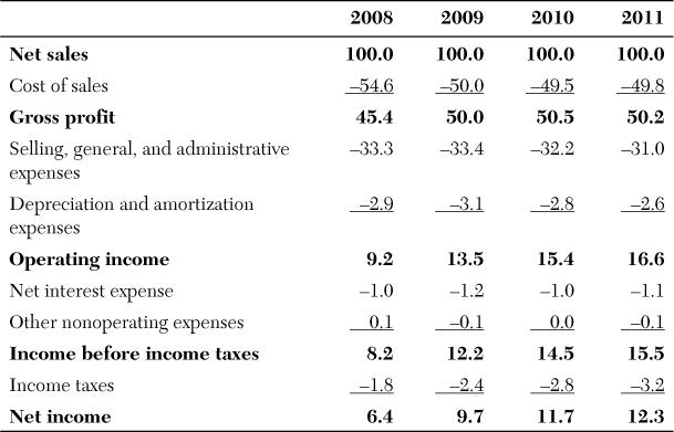
Exhibit 2.4 reveals the following:
• Mattel’s net income as a percentage of net sales (the net profit margin) grew from 6.4 percent in 2008 to 12.3 percent in 2011, as previously observed in Exhibit 2.3.
• The cost of sales, also known as the cost of goods sold, declined from 54.6 percent in 2008 to 49.8 percent in 2011, accounting for a 4.8 percentage point increase in profitability.
• Selling, administrative, and general expenses (SG&A) declined from 33.3 percent in 2008 to 31.0 percent in 2011, accounting for a 2.3 percentage point increase in profitability.
• Net interest expense, which is the difference between the interest expense on the amounts borrowed and the interest income of the amounts invested, remained low and stable throughout the period, representing between 1.0 and 1.2 percent of net sales.
• Income taxes increased year on year, absorbing 1.8 percent of net sales in 2008 and 3.2 percent of net sales in 2011.4
As this analysis of Mattel’s common-size income statement data reveals, decomposing the net profit margin enables the analyst to address the following questions:
• Is the target’s net profit margin changing over time? If so, which factors are causing the changes: cost of sales, SG&A, interest costs, income taxes, or other costs? By identifying the factors that affect the company’s profitability, the analyst gains a better understanding of the company’s cost structure, which proves useful when attempting the pro forma analysis.
• How well is the target managing its costs of doing business? Has it reached sufficient volume levels to gain any economies of scale? In which areas, if any, does the target seem to be overspending?
1.2.2. Decomposing Asset Turnover
Asset turnover, or what is sometimes called asset management, refers to the degree of productivity that a company is able to achieve with respect to its assets. It is a measure of the effectiveness with which a company’s management can employ the valuable resources provided by creditors and owners alike. Not surprisingly, a strong link exists between the effective use of a company’s assets and its degree of profitability.
Exhibit 2.3 showed that, in 2011, Mattel generated 12.3 cents in net income from each dollar of sales revenue, while generating $1.13 in sales revenue from each dollar of assets. Mattel can increase shareholder value either by increasing the rate of profit per dollar of sales revenue or by increasing the volume of sales revenue generated from its existing investment in assets.
The decomposition of the total asset turnover traditionally focuses on two groups of assets that are closely related to the company’s operations: (1) working capital, which includes operating assets such as trade receivables and inventories, and operating liabilities such as trade payables; and (2) the noncurrent revenue-producing assets such as property, plant, and equipment (PP&E). To determine how effectively management has used a company’s asset base, analysts usually calculate the following ratios.
Working Capital Ratios:
A measure of the number of production cycles (production of inventory from raw materials to finished goods → inventory → sale of inventory to customers) occurring in a given period of time (usually one year or one quarter).
A measure of the number of days, on average, needed to sell the existing inventory, calculated on an annual basis.

A measure of the number of accounts receivable collection cycles (sale of inventory to customers on credit → accounts receivable → cash collection from customers) occurring in a given period of time.
A measure of the number of days, on average, required for collecting an outstanding account receivable, calculated on an annual basis.

A measure of the number of account payment cycles (buy inventory from suppliers on credit → accounts payable → cash payment to suppliers) occurring in a given period of time.
A measure of the number of days, on average, required for paying an outstanding account payable, calculated on an annual basis.
Noncurrent Assets Ratios:

A measure of the value of net sales generated for a given investment in noncurrent assets.
Property, Plant, and Equipment Turnover =

A measure of the value of net sales generated for a given investment in PP&E.
Several observations about the preceding ratios are noteworthy. First, not all of these ratios are relevant for all companies. For example, McDonald’s, a worldwide chain of fast-food restaurants, maintains an insignificant balance in accounts receivable. Few, if any, of the company’s sales are undertaken on a credit basis. Thus, analyzing the accounts receivable turnover for a company such as McDonald’s is unnecessary. Second, some of the ratios are merely transformations of other ratios. For instance, the days of inventory on hand is only a transformation of the inventory turnover. Analysts often do not need to calculate both ratios, although many do. Third, for assets, a high rate of turnover is better than a lower rate; for liabilities, it is the opposite. For example, higher inventory and accounts receivable turnover ratios are desirable because they indicate shorter production and collection cycles, respectively. Shorter production and collection cycles minimize the investment in working capital. In contrast, lower accounts payable turnover ratios are preferable because the longer the company has to pay its suppliers, the better. This generality is true except when management is liquidating its revenue-producing assets (a dangerous situation for any company in the long run). Finally, the previous set of ratios should not be considered exhaustive; analysts frequently add to and subtract from the previous list.
Exhibit 2.5 shows Mattel’s working capital and noncurrent ratios for the period 2008–2011.

Exhibit 2.5 reveals the following:
• The inventory turnover fluctuated slightly, from 7.07 times in 2008, down to 6.45 times in 2009, back up to 7.08 times in 2010, and back down to 6.56 times in 2011. Symmetrically, the number of days of inventory on hand oscillated between 52 days in 2008 and 2010, and 56 and 57 days in 2009 and 2011. Overall, Mattel’s inventory management deteriorated slightly throughout the four-year period. This deterioration partly explains the decline in the total asset turnover between 2008 and 2011 in Exhibit 2.3.
• The accounts receivable turnover fell from a high of 6.69 times in 2009 to a low of 5.24 times in 2011. In parallel, the cash collection period increased: Mattel was taking 55 days to collect from its customers in 2009, but 15 more days in 2011. This deterioration of the receivable collection cycle also contributed to the decline in the total asset turnover between 2008 and 2011.
• The accounts payable turnover rose from a low of 7.03 times in 2009 to a high of 8.42 times in 2011. Symmetrically, the cash deferral period decreased: Mattel took 52 days to pay its suppliers in 2009, but 9 days less in 2011.
• In 2009, Mattel took about the same amount of time to pay its suppliers (52 days) that it took it to collect from its customers (55 days). Two years later, it was paying its suppliers 13 days faster than it was collecting from its customers. The simultaneous decrease in the cash deferral period and increase in the cash collection period had a negative effect on Mattel’s working capital.
• The PP&E turnover grew from 10.43 times in 2009 to 12.42 times in 2011. This increase in sales revenue given Mattel’s asset base indicates that the company improved the efficiency of its PP&E. That had a positive effect on its total asset turnover, its ROA, and, ultimately, its ROE.
1.2.3. Decomposing Financial Leverage
Financial leverage reflects a company’s ability to increase its performance through borrowing. Debt can be a powerful tool for enhancing shareholder value, but the effectiveness of financial leverage is directly related to the spread between a company’s cost of borrowing and the return on those borrowed funds. As this spread declines, the ability of financial leverage to enhance shareholder value also declines.
A company’s financial leverage affects its ability to service its debt (make interest payments) and repay it. As financial leverage increases, so does financial risk. A company with low financial risk (a high ability to make interest payments and repay its debt) can borrow at a lower cost than a company with high financial risk. In general, increases in the amount of financial leverage are more effective in enhancing shareholder value for companies with low financial risk than for companies with high financial risk. Thus, analysts who want to evaluate the extent and effectiveness of financial leverage often analyze a company’s financial riskiness. Their analysis typically focuses on two dimensions of financial riskiness: short-term risk, or liquidity, and long-term risk, or solvency.
For most companies, the following ratios are calculated when financial risk is analyzed.
Liquidity Ratios:

A measure of the highly liquid current assets available for repaying short-term liabilities.5
A measure of the cash flow from operations available for repaying short-term liabilities.
Solvency Ratios:

A measure of the relative investment of all creditors versus common shareholders.

A measure of the relative investments of long-term creditors, usually financial institutions and financial markets, versus common shareholders.
A measure of the extent to which current operations can support current debt service charges.
Three observations about these ratios are useful. First, the higher the liquidity and the interest coverage ratios, and the lower the total liabilities-to-equity and long-term debt-to-equity ratios, the lower the financial risk. Second, the short-term liquidity ratios focus on the two sources of liquid resources that are immediately available to managers: cash on hand and other highly liquid current assets (quick ratio) or cash flows from operating activities (operating cash flow ratio). However, a company’s short-term obligations can be repaid with cash generated from a variety of other sources: future operations, the sale of assets, the issuance of stock, or new borrowings. Third, the long-term solvency ratios focus on two separate aspects of risk: (1) the company’s existing level of financial leverage (total liabilities-to-equity ratio and long-term debt-to-equity ratio) and (2) the ability of a company to cover the current cost of debt from the income its existing operations generate. If a company is already highly leveraged, additional borrowings will not be as effective in enhancing shareholder value. As stated earlier, as the degree of financial leverage increases, so does a company’s riskiness. Lenders charge commensurately higher interest costs, thereby reducing the utility of additional borrowings.
Exhibit 2.6 shows Mattel’s liquidity and solvency ratios for the period 2008–2011.
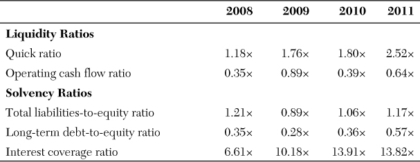
Exhibit 2.6 reveals the following:
• With respect to liquidity, the quick ratio increased from 1.18 times in 2008 to 2.52 times in 2011, and the operating cash flow ratio increased from 0.35 times in 2008 to 0.64 times in 2011. Both ratios indicate that Mattel’s liquidity improved throughout the four-year period.
• With respect to solvency, the total liabilities-to-equity ratio and the long-term debt-to-equity ratio both indicate a decrease in financial leverage between 2008 and 2009, and a subsequent increase in financial leverage between 2009 and 2011. Overall, the first ratio shows a slight decrease in total liabilities relative to shareholders’ equity throughout the period, whereas the second ratio indicates a slight increase in long-term debt compared to shareholders’ equity. Put another way, the relative investment of financial institutions and financial markets among creditors rose between 2009 and 2011. However, the interest coverage ratio improved during the period, with the amount of operating income being 13.82 times higher than the amount of interest expense in 2011, versus 6.61 times higher in 2008.
As illustrated in Exhibit 2.3, Mattel’s financial leverage did not change much between 2008 and 2011. Thus, the joint effect of liquidity and solvency was close to neutral, indicating that the company’s financial riskiness remained stable.
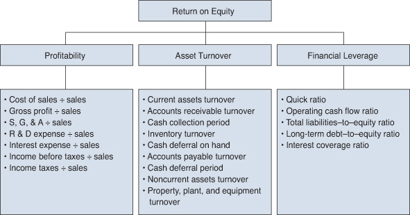
1.2.4. Analytical Framework: Putting It All Together
Exhibit 2.7 presents an integrative framework for the ratio analysis of a target. The framework is premised on the notion that the primary goal of corporate management is to maximize shareholder value. As such, the cornerstone of the model is a company’s ROE. As discussed earlier, the ROE can be decomposed into the three key drivers of profitability, asset turnover, and financial leverage. Each of these three key drivers can be decomposed into various subcomponents. This ratio analysis helps analysts understand the drivers of the target’s performance, which proves useful when starting the pro forma analysis that leads to the target’s valuation.
1.3. Cash Flow Analysis
With the exception of the operating cash flow ratio, all ratios discussed thus far are derived from the income statement and the balance sheet. Given that cash flows are an important consideration for investors, any financial review should include an analysis of cash flows. Therefore, the analyst should analyze the target’s cash flow statement. The structure of the cash flow statement typically includes three categories:
• Cash flows from operating activities
• Cash flows from investing activities
• Cash flows from financial activities
The cash flow from operating activities (CFFO) represents the cash generated from the sale of goods or services minus the cash paid for operations—in essence, net income on a modified cash basis. The cash flow from investing activities (CFFI) represents the cash paid for investments (both short-term and long-term), the cash paid for new capital expenditures, and the cash received from the sale or disposal of noncurrent assets. Finally, the cash flow from financing activities (CFFF) represents the cash generated from raising funds, either via short-term or long-term borrowings or through the issuance of stock, minus the cash paid for retiring debt, repurchasing shares, or paying dividends.
Cash flow analysis enables the analyst to address a variety of key questions, such as the following:
• Is the target generating a positive CFFO? If so, is it also generating a positive discretionary cash flow?
• What types of strategic investments has the target been making?
• How has the target been financing its operations and its strategic investments?
• How has the target financed the cash distributions to shareholders, namely dividend payments and share repurchases?
A company’s discretionary cash flow is the amount of cash remaining from the CFFO after all required cash needs are deducted. It is defined as follows:
Discretionary cash flow = CFFO − Debt repayments − Dividend payments − Capital expenditures to replace used-up property, plant, and equipment6
If the discretionary cash flow is positive, it represents the surplus of cash that management has at its disposal to undertake some discretionary act (such as retire debt early, repurchase shares, or make intercorporate investments) without relying on additional external funding. Alternatively, a negative discretionary cash flow indicates that the company does not generate sufficient cash from its operations to fund its growth. Unless it is a temporary situation, a negative discretionary cash flow is usually the sign of a struggling company with structural problems. In addition, it is not uncommon for companies that consistently have a negative discretionary cash flow to increase financial leverage to get the cash required to make interest payments and debt repayments, or to finance the necessary investment to replace used-up PP&E. Raising more debt to stay afloat is not sustainable in the long run, particularly if the company’s financial risk reaches such a high level that lenders either charge the company more for the funds it borrows or cease to lend altogether.
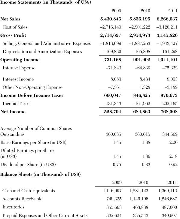
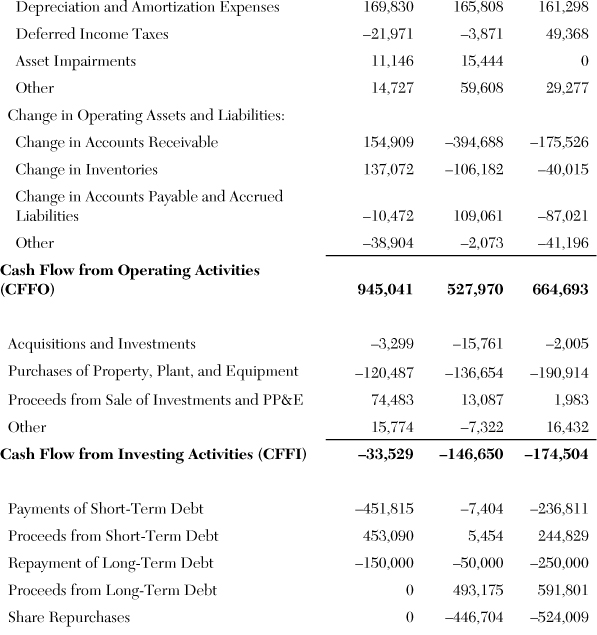
To illustrate cash flow analysis, consider Exhibit 2.8, which contains Mattel’s cash flow statement for the period 2009–2011.
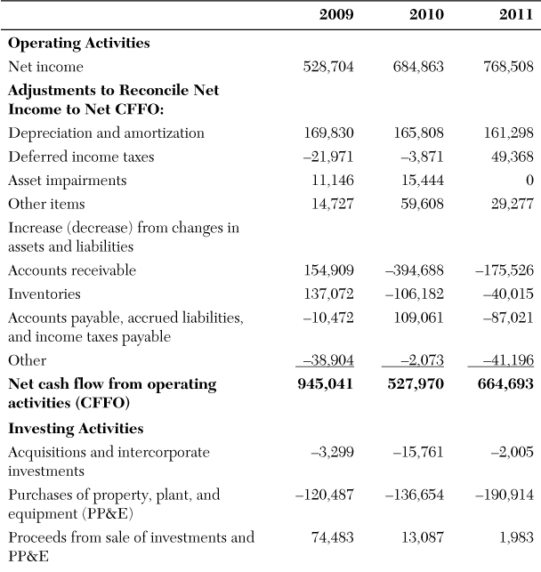
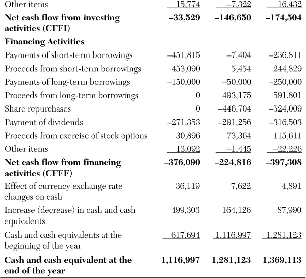
Exhibit 2.8 reveals the following:
• Mattel generated a positive CFFO of $945.0 million in 2009, $528.0 million in 2010, and $664.7 million in 2011. The CFFO in 2009 was exceptionally high because of a large reduction in working capital. As the amount of cash tied up in inventories and accounts receivable decreased, the CFFO increased. However, this reduction in working capital, which might have been a consequence of the global economic slowdown, was temporary, which explains why the CFFO in 2010 and 2011 went back to its “normal” level.
• The CFFI was negative for each of the three years, ranging from –$33.5 million in 2009 to –$174.5 million in 2011. The company made significant investments in new PP&E, reaching $190.9 million in 2011. It also made acquisitions, although the amounts spent on acquisitions remained small relative to its investments in PP&E. In 2010, Mattel bought intellectual property rights for $15.8 million. All these investment outlays were only partially offset by the proceeds generated from the disposal of select investments and PP&E, which were limited to $2.0 million in 2011.
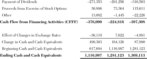
• The CFFF was negative for each of the three years, indicating that Mattel distributed more cash than it raised. In 2009, the company reduced its debt outstanding by $148.7 million—it repaid $150 million of long-term borrowings, and short-term borrowings increased by only $1.3 million. In contrast, during the following two years, Mattel increased its borrowings, raising an additional $441.2 million in 2010 and $349.8 million in 2011. This is consistent with the increase in the long-term debt-to-equity ratio noted in Exhibit 2.6. Mattel also distributed cash to its shareholders. Dividend payments increased from $271.3 million in 2009 to $316.5 million in 2011. During the same period, the number of shares declined, as the company repurchased shares—nearly $1 billion in 2010–2011. Thus, the dividend per share increased, from $0.75 in 2009 to $0.92 in 2011.
• Overall, the cash balance more than doubled in three years, from $617.7 million at the beginning of 2009 to $1.4 billion at year-end 2011. Not only was Mattel able to grow its business and honor its contractual obligations, but it also managed to reward its owners regularly and significantly and maintain a healthy cash balance.
The analysis of Mattel’s cash flow statement also illustrates two interesting facts. First, companies need to adjust their operating, investing, and financing activities in response to economic conditions. Many countries experienced a slowdown or even a recession in the years following the global financial crisis that started in 2008. As shown in Appendix 2A, Mattel’s sales revenue contracted in 2008 and 2009. However, the company managed to maintain (and even increase) its profitability by cutting operating expenses and, as mentioned earlier, releasing cash from its working capital requirement. As shown in Exhibit 2.8, it also saved cash by suspending its share repurchase program. Second, management tends to be opportunistic, particularly when it comes to financing decisions. Mattel took advantage of low interest rates, credit rating upgrades, and investors’ appetite for investment-grade debt issuances to increase its borrowings in 2010 and 2011.7 It raised $500 million in September 2010 ($493.2 million net of issuance costs) and $600 million in November 2011 ($591.8 million net of issuance costs).
What about Mattel’s discretionary cash flow? It would be inaccurate to estimate it by subtracting from the CFFO the entire short-term and long-term debt repayments, dividend payments, and purchases of PP&E because not all these amounts are required cash needs. For example, some purchases of PP&E might not be intended to replace used-up noncurrent assets, but instead might be used to expand the business. Although there is a tacit agreement with shareholders that the dividend should be maintained, Mattel did not have to increase it by 10.8 percent between 2010 and 2011 (from $0.83 to $0.92 per share). A review of the footnotes to the financial statements also indicates that Mattel had a required repayment of $250 million of long-term borrowings in 2011, but that it had more flexibility regarding its short-term borrowings: In the unlikely event that the company could not roll over (refinance) its short-term borrowings, it had the ability to use a $1.1 billion credit facility.
Exhibit 2.9 provides a more realistic estimate of the discretionary cash flow for 2011. It is assumed that the debt repayment is limited to the required repayment of $250 million; that the dividend is maintained at $0.83 per share, or $285.5 million, based on the number of shares outstanding in 2011; and that the required purchases of PP&E are equal to the amount of depreciation for the year ($147.5 million).

Mattel’s discretionary cash flow is negative, primarily because of the large debt repayment that was due in 2011. A review of the footnotes indicates that the future debt repayments are $50 million in 2012, $400 million in 2013, $0 in 2014 and 2015, and $300 million in 2016. Thus, provided that Mattel can maintain or grow its CFFO, the level of discretionary cash flow should be positive in 2012, 2014, and 2015, but could be negative in 2013 and 2016.
To conclude the financial review of Mattel, the Exhibit 2.10 provides excerpts of the report that Fitch, one of the leading credit rating agencies, released when it reviewed the company in October 2012. This report reinforces some of the financial issues discussed thus far.
Exhibit 2.10 Operating Section of Mattel’s Historical and Projected Income Statements

Amounts are in millions of $, and common sizes are in percentages. SG&A = selling, general and administrative. D&A = depreciation and amortization expenses
With the historical financial review complete, we now turn to the task of developing forecasts for a company.
2 Pro Forma Analysis
After completing the historical financial review, the analyst is ready to begin developing forward-looking pro forma financial statements. Inherent in the process of developing pro forma financial statements is the necessity for the analyst to make numerous assumptions about events that have not yet occurred. If the analyst is to avoid overvaluing the target, it is imperative that he or she bases all assumptions on sound logic and reasoning. When such assumptions are not well conceived, the cost to an acquirer can be quite significant, as illustrated in the vignette at the beginning of this chapter.
2.1. Pro Forma Financial Statements
We start by identifying the steps necessary to develop pro forma financial statements. Then we apply the process to Mattel.
2.1.1. Process
The preparation of pro forma statements is typically a six-step process:
1. Forecast the target’s sales revenue. The projection of future sales is unquestionably the most important step in the pro forma process. Because it is the starting point of the pro forma analysis and the valuation of a target, a misestimation at this stage is compounded into a multitude of other forecast amounts. In general, sales are forecast for three to five years, and possibly for as long as ten years. Most analysts are reluctant to forecast beyond five years, however, largely because of the high likelihood of error in long-term forecasts. Because most companies have a continuing value beyond the final forecast year, the analyst must also project a value of the business for all the years subsequent to the final forecast year. This value is known as the continuing value, terminal value, or exit value. Chapter 3, “Traditional Valuation Methods,” covers the process of estimating this value.
2. Forecast the target’s operating expenses (excluding financing costs). Projecting operating expenses includes preparing forecasts for the cost of sales, SG&A, and other continuing income and expense accounts. These forecasts should include the effects of any anticipated cost reductions or economies of scale expected to arise as a consequence of the acquisition.9
Some operating expenses are relatively easy to forecast because either they are fixed in amount or they vary as a function of revenues. In contrast, other operating expenses are more difficult to project because they are neither strictly fixed nor strictly variable. A good source of information to forecast operating expenses is the historical common-size income statements. For operating expenses that vary in a relatively constant relationship with sales, as revealed by a multiyear common-size statement analysis, the common-size percentage can be a useful way for an analyst to forecast these expenses in future periods.
3. Forecast the asset side of the balance sheet. Forecasting assets can be done in one of two ways: (1) Forecast total assets and then allocate this total among the individual asset accounts using the common-size balance sheet percentages (and potentially other assumptions), or (2) forecast the individual asset accounts and then sum the accounts to arrive at a value for total assets. The first approach is more frequently used, largely because of its ease. It usually assumes that most companies maintain a relatively constant relationship between sales and total assets (a constant total asset turnover ratio). The individual asset accounts are then forecast by reference to various assumptions about the growth (or decline) in the various asset accounts and to a target’s most recent common-size balance sheet.
The second approach to forecasting assets is more complex but somewhat more refined. For example, it is reasonable to expect that the level of PP&E relative to sales will decline with small increases in sales, particularly if the company has unused capacity. In contrast, working capital as a percentage of sales tends to remain relatively fixed—increases in sales are often accompanied by increases in inventories and accounts receivable. These expected relationships are more easily incorporated in the pro forma balance sheet with the second approach.
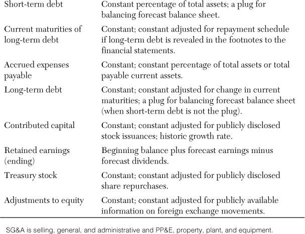
4. Forecast the liabilities and equity side of the balance sheet. As part of this step, the analyst needs to forecast the target’s long-term financing, including any net proceeds from the issuance versus retirement of long-term debt and any net proceeds from the issuance versus repurchase of shares. The target’s future dividend policy, if any, should also be reflected in the forecast.
At this juncture, it is appropriate for the analyst to deal with the question of cash surpluses and deficits relative to the cash balance forecast in step 3. Most companies maintain bank lines of credit, so one useful assumption is to increase the amount of short-term debt for any cash deficit relative to the step 3 forecast. If there is a cash surplus, the analyst can decrease the amount of short-term debt, if any, or increase the amount of cash.10
5. Complete the pro forma income statement and balance sheet by forecasting net interest expense (interest expense minus interest income) and income taxes.
6. Derive the pro forma cash flow statement. At the end of this chapter, Appendix 2B presents a methodology for preparing a cash flow statement from balance sheet and income statement data.11
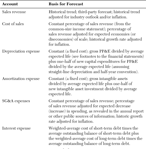
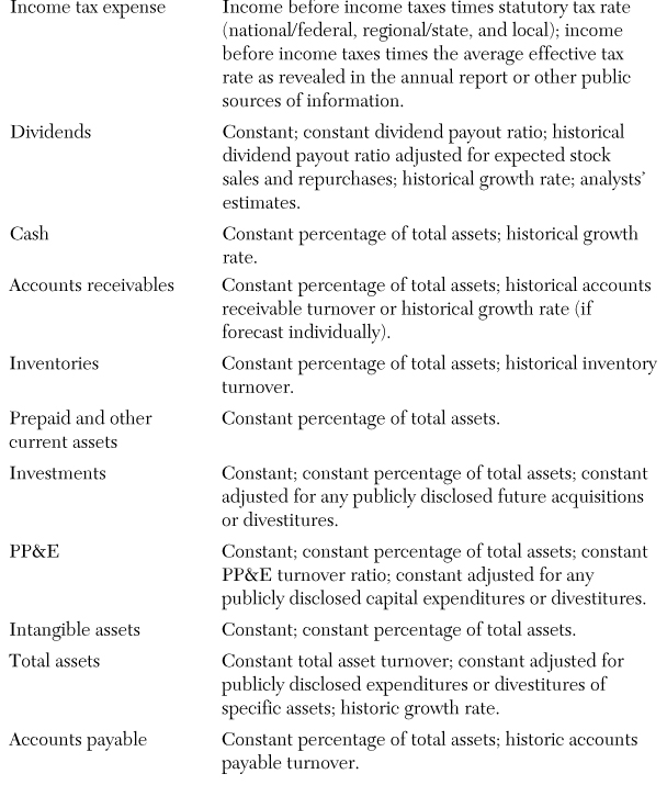
Appendix 2C contains alternative approaches to forecasting the various income statement and balance sheet accounts.
Building a complete set of detailed forward-looking pro forma financial statements is a time-consuming exercise that requires not only a good understanding of the company’s business and environment, but also strong accounting skills. Some financial statement accounts are relatively easy to forecast. For example, sales revenue at the company or division level can be forecast by multiplying the sales revenue for the current year by one plus the projected growth rate. Under normal circumstances, the cost of sales and working capital accounts tend to vary little relative to sales, and it is not uncommon for management to indicate the amount that will be spent as capital expenditures in the coming year.
In contrast, other financial statement accounts are far more difficult to forecast. A challenge analysts typically face is to project accounts that are rather unstable over time. Financial statement accounts that depend on volatile macroeconomic variables are particularly challenging to forecast. For example, developing the pro forma financial statements of a multinational company whose sales revenue and operating costs are generated in different currencies requires forecasting exchange rates, a highly challenging and unreliable endeavor. Some of the financial statement accounts might also be unpredictable because they reflect discretionary management decisions. For instance, accurately predicting the timing and amount of acquisitions or share repurchases is difficult. An additional challenge is forecasting financial statement accounts that are affected by a multitude of factors, including accounting and tax considerations. For example, developing a pro forma balance sheet requires forecasting accounts such as deferred tax assets or liabilities and accumulated other comprehensive income, two accounts that require a solid understanding of accounting standards and tax codes.12
Sell-side analysts typically develop detailed forward-looking pro forma financial statements and include a condensed version in their research reports. In doing so, they help potential investors assess a company’s future performance before buying the company’s debt or equity securities. In the context of M&As, however, pro forma analysis is only a preparatory step to value the target; it is a means for the acquirer and its adviser to determine what the target is worth, a critical step in setting the offer price and assessing whether the acquisition has the potential to create value. Thus, valuation analysts generally forecast only the financial statement accounts that are necessary to estimate the target’s value. Instead of spending time projecting accounts that have little effect on their valuation, such as noncash items or shareholders’ equity, analysts focus on the key drivers of the target’s value. They often complete only the first two steps of the six-step process described earlier, focusing on the forecast of sales revenue and operating expenses that represent the core of the target’s earnings and cash flows and, thus, value. Depending on the valuation method they use, they might also address part of the other steps, such as forecasting the target’s working capital accounts (step 3), the effect of long-term financing (step 4) on key accounts (such as short-term debt, long-term debt) and financial leverage, or the amount of interest expense (step 5). Thus, valuation analysts rarely end up with a full set of detailed, forward-looking financial statements.
2.1.2. Illustration
We now return to Mattel, to illustrate some types of forecasting and modeling decisions inherent in preparing a company’s valuation. We focus on forecasting the financial statement accounts that are necessary to estimate the company’s value—primarily the income statement, which requires forecasting sales revenue (step 1), operating expenses (step 2), and net interest expense and income taxes (steps 4 and 5). We also illustrate how to use ratios to forecast PP&E and working capital accounts (step 3).
Step 1
To forecast Mattel’s sales revenues, it is necessary to make an assumption about the growth rate in sales between 2011 and 2012. Between 2008 and 2011, Mattel’s sales revenues grew by approximately 6 percent (about 2 percent per year), but that period included two years of global economic slowdown and sales declines for Mattel. The growth rate in sales between 2010 and 2011 was stronger, at approximately 7 percent, but it could have been exceptionally high due to the economic recovery that took place in many countries where Mattel sells its toys. For the purpose of our illustration, we use an intermediate growth rate of 3 percent.
Step 2
To forecast Mattel’s operating expenses, we use the common-size income statement percentages from 2011. This assumption presumes that all of the company’s operating expenses move in a constant proportion to net sales, which is unlikely the case. However, it is a valid assumption for at least some of Mattel’s operating expenses (such as the cost of sales), and such an approach is appropriate when operating expenses are relatively stable over time.13
Exhibit 2.10 shows the operating section of Mattel’s historical income statements for 2010 and 2011. The shaded areas show the forecast amounts for 2012.
To support the growth forecast in Exhibit 2.11, Mattel will likely have to invest in additional assets, both PP&E and working capital. We use the PP&E turnover ratio for 2011 to forecast PP&E in 2012. Based on a PP&E turnover ratio of 12.42 times in 2011 and a forecast amount for net sales of $6,454.0 million, the average PP&E is $519.5 million. PP&E at year-end 2011 was $523.9 million, which means a forecast amount for PP&E at year-end 2012 of $515.0 million. Similarly, to forecast Mattel’s accounts receivable, inventory, and accounts payable, we use the working capital ratios for 2011.
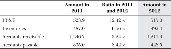
Exhibit 2.11 shows the historical and forecast amounts of Mattel’s PP&E and working capital accounts for 2011 and 2012, respectively.
To be able to forecast Mattel’s interest expense, we must make an assumption about the ending balance of interest-bearing debt (short-term debt and long-term debt) in 2012. The historical balance sheets in Appendix 2A and a review of the footnotes indicate that Mattel makes little use of its bank lines of credit. We assume that this situation will not change and that the ending balance for short-term debt in 2012 will be the same as in 2011 ($8.0 million).
Companies usually provide details about their long-term borrowings in the footnotes to the financial statements, including the repayment schedule for their debt. This schedule can be used to forecast a company’s debt retirements. However, a company’s capital structure tends to be stable—the debt that comes due is often rolled over, to maintain a relatively constant financial leverage. Unless the company is involved in a transaction that has a significant effect on its capital structure, such as an LBO, it is generally realistic to assume that the amounts of debt issuance and retirement will balance each other out. Because there is no evidence that Mattel is aiming to either increase or decrease its borrowings significantly, we assume that the amount of long-term debt due to be repaid in 2012 ($50 million) will be refinanced. Thus, the ending balance for long-term debt will not change between 2011 and 2012 and will remain at $1.5 billion.
When forecasting a company’s long-term financing, the analyst must also make assumptions about any issuances or repurchases of shares and about the company’s dividend policy. The historical cash flow statements in Exhibit 2.8 reveal that Mattel has not issued any common shares to the public for the last three years, and it is highly unlikely to do so in 2012. However, the company repurchased shares to return cash to its shareholders and to neutralize the effect of its stock option plans. Thus, as long as Mattel continues generating more cash than it needs to reinvest internally to grow its business, it will likely continue repurchasing shares. We assume that the company will repurchase in 2012 an amount similar to that repurchased in 2010 and 2011 (approximately $400 million to $500 million). At a minimum, Mattel will also maintain its dividend per share (and perhaps increase it slightly). Thus, we assume a dividend payment of approximately $320 million in 2012.14
To complete Mattel’s pro forma income statement, two final items need to be forecast: net interest expense and income taxes. With respect to interest expense, the following equation is needed:

where I refer to the interest rate on the amounts borrowed (the average cost of debt), STD to short-term debt, LTD to long-term debt, B to the balance at the beginning of the period, and E refers to the balance at the end of the period. This equation assumes that a company’s interest expense is a function of its beginning and ending balances of debt, which are averaged to reflect the level of debt throughout the year.15
A review of Mattel’s footnotes indicates that the company’s weighted average cost of debt in 2011 was 0.4 and 6.9 percent for short-term and long-term debt, respectively. Given forecasts of relatively stable interest rates for 2012, we assume that Mattel’s cost of debt will remain unchanged. Therefore, the previous equation becomes:
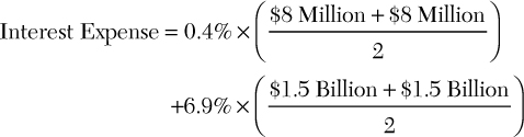
which gives an interest expense of $103.5 million.
Mattel also invests its cash balance and receives interest income on these investments. Interest income can be estimated as follows:
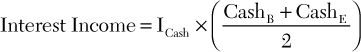
where ICash refers to the interest rate on the amounts invested (average yield), and CashB and CashE refer to the balance at the beginning and end of the period, respectively.
The ending cash balance at this stage is unknown because it is one of the last accounts to be forecast. Indeed, the amount of cash left on a company’s balance sheet at the end of the period is the net result of all the cash inflows and outflows during the period; until all these cash flows have been forecast, the ending cash balance cannot be determined accurately. An analyst who develops a full set of detailed pro forma financial statements returns to forecasting this account when his or her pro forma analysis is close to completion. As mentioned earlier, our objective in this illustration is to prepare the ground for the valuation of Mattel and to focus on the key accounts that drive this valuation. A review of Mattel’s balance sheets over the last three years indicates that the ending cash balance has increased from $1.1 billion in 2009 to $1.4 billion in 2011. Mattel likely will adjust its operating, investing, and financing decisions accordingly to maintain this trend: Financial markets value predictability, and a company such as Mattel aims to maintain a balance between the level of its ending cash balance and the level of its cash distributions to shareholders. In addition, in a low-interest-rate environment where cash investments yield little, a slightly inaccurate forecast for the ending cash balance will have a limited effect on the company’s value. Because the yield on cash investments is also unknown, we assume for simplicity that the interest income remains constant between 2011 and 2012, at $8.1 million.
To forecast income taxes, we assume that the company’s effective tax rate (income taxes divided by income before tax) remains constant between 2011 and 2012, at 20.8 percent.16
Exhibit 2.12 builds from Exhibit 2.10 and presents Mattel’s historical and projected income statements for the period 2010–2012.17
Exhibit 2.12 Mattel’s Historical and Projected Income Statements
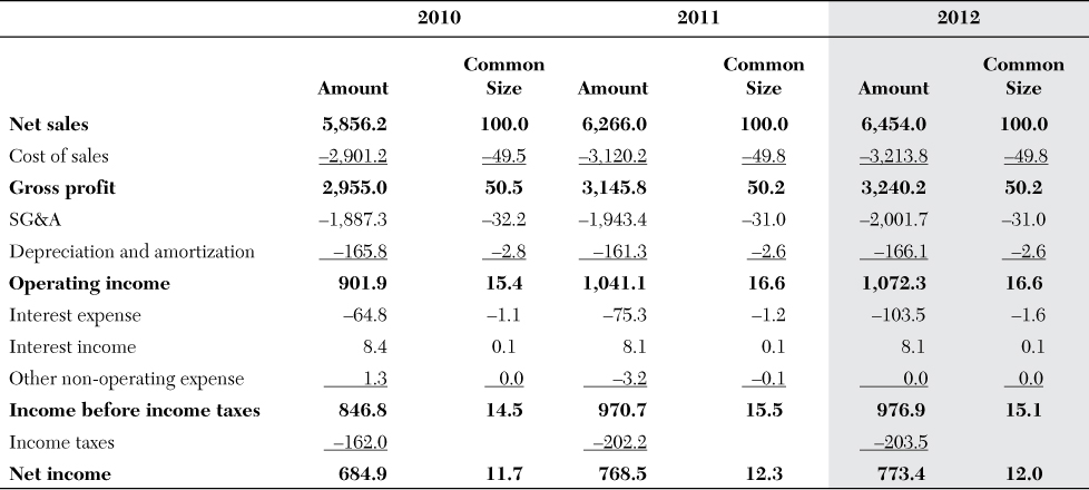
Amounts are in millions of $, and common sizes are in percentages.
Based on our assumptions, Exhibit 2.12 shows that Mattel’s net sales, gross profit, and operating profit are expected to increase by 3 percent, in line with the growth rate in sales between 2011 and 2012. The increase in net income is limited to 0.6 percent only, primarily because of the assumption that the amount of debt will remain constant at a level that is slightly higher than historically, thus leading to a higher interest expense.
2.2. Sensitivity, Scenario, and Monte Carlo Simulation Analyses
Pro forma analysis reflects a set of assumptions about a series of events that have not yet occurred. What if the analyst lacks confidence about one of his or her assumptions and wants to assess how a change in this assumption would affect his or her forecast? In our case, perhaps we want to investigate the effect that a lower growth rate in sales or a different ending balance for long-term debt would have on net income. After the model has been built in Excel, performing sensitivity analyses is straightforward—we can assess the effect of changes in one input at a time (such as the growth rate in sales) on selected outputs (such as operating income and net income). Exhibit 2.13 shows the result of such a sensitivity analysis, from a sales contraction of 10 percent (in line with the 8 percent sales contraction that Mattel experienced between 2008 and 2009) to a sales expansion of 10 percent.

Exhibit 2.13 shows that if Mattel does not experience any growth in sales between 2011 and 2012, its operating income will remain unchanged, at $1,041.1 million. Net income, however, will fall by 3.2 percent to $748.7 million, primarily because of the additional amount of borrowing in 2012 relative to 2011. To maintain net income at $768.5 million, Mattel must grow the top line by 2.4 percent, with all else equal.18
Rerunning the pro forma analysis for multiple values of the various key inputs can be time consuming. Thus, some analysts prepare only three separate scenarios involving the key assumptions: a most likely scenario, an optimistic scenario, and a pessimistic scenario. In our case, the pro forma income statement in Exhibit 2.13 reflects our most likely scenario. We could present a pro form income statement for a sales expansion of 10 percent (optimistic scenario) and a pro forma income statement for a sales contraction of 10 percent (pessimistic scenario).
Scenario analysis is certainly less time intensive because it requires only a limited number of iterations of the forecast model; however, it is not always without cost because the dynamic interaction of the key inputs cannot be rigorously explored. For this reason, analysts are increasingly turning to Monte Carlo simulation analysis to fully explore how the key inputs jointly affect the forecast amounts. Add-ins to Excel such as Oracle Crystal Ball, Palisade @Risk, Vose ModelRisk, and Frontline Risk Solver offer analysts a relatively straightforward way of performing Monte Carlo simulations.
Although sensitivity, scenario, and Monte Carlo simulation analyses can be tedious, they give the analyst critical insight regarding the relative importance of each assumption. They also allow analysts and executives to gain a better understanding of what drives a company’s performance and value. This exercise is helpful in preventing analysts from overvaluing a target and corporate executives from overpaying for their acquisitions. This is paramount in avoiding the winner’s curse.
Summary
In this chapter, we considered the related processes of financial review and pro forma analysis. Financial review refers to the process of analyzing and understanding the financial history of a target, which is an integral part of the due diligence investigation that should precede any acquisition. Financial review also provides essential inputs for the preparation of forecasts that are necessary to value the target. Although important valuation considerations include selecting an appropriate discount rate or valuation multiple, nothing is more important in assessing the target’s value than an accurate modeling of its operations and drivers of performance. In Chapter 3, we link the construction of pro forma analysis to our ultimate goal of assessing a company’s value.
Endnotes
1. For convenience, we assume from this point that companies have only common stock outstanding, and hence we ignore preferred stock dividends. Except for financial institutions, few companies have preferred stock in their capital structure. When they do, the amount of preferred stock is usually small relative to the amount of common stock. Financial institutions, particularly deposit-taking institutions, use preferred stock because of capital requirements imposed by the regulators. For example, the Basel Capital Adequacy Accords allow banks to include in core capital (the measure of a bank’s financial strength) nonredeemable, noncumulative preferred stock.
2. Some analysts question the internal consistency of the ROA as a measure of profitability. Their concern stems from the fact that the income statement deducts an opportunity cost for debt (interest expense) but makes no similar deduction for the opportunity cost of equity. These analysts believe that a more consistent measure of profitability is given by the unleveraged ROA, or UROA:
UROA is a measure of profitability before interest charges. The adjustment for taxes is designed to recognize the tax benefit resulting from the interest expense deduction. Another refinement some analysts use is to replace total assets with the sum of shareholders’ equity and interest-bearing debt. In doing so, they eliminate those assets obtained through non-interest-bearing debt. This refinement creates a measure called return on net assets (RONA):
3. All the calculations in this book were performed in Excel, without rounding any of the intermediate results. As a consequence, slight differences might arise between the numbers reported and the ones obtained with a calculator.
4. A better way to assess a company’s tax burden is to calculate the effective tax rate, where income taxes are divided by the income before income taxes rather than net sales. Mattel’s effective tax rate decreased from 22.2 percent in 2008 to 19.1 percent in 2010, but increased to 20.8 percent in 2011.
5. A close variant of the quick ratio is the current ratio, measured as current assets divided by current liabilities. The quick ratio is generally preferred to the current ratio because the current ratio includes all current assets, some of which, such as inventories and prepaid expenses, are not always liquid.
6. Discretionary cash flow is not to be confused with free cash flow, which is discussed in Chapter 3. Why debt repayments and capital expenditures to replace used-up PP&E are required cash needs is obvious. Interest payments and debt repayments are contractual obligations, and a company that misses interest payments and debt repayments would default, which could lead to liquidation in an extreme case. A company that does not replace used-up PP&E would harm its business and fairly quickly become unable to operate. In addition, it is not uncommon for lenders to impose covenants, clauses that specify what the borrower can (positive covenants) and cannot (negative covenants) do. A standard covenant is the obligation to insure and maintain the asset base. Dividend payments, in contrast, are not contractual obligations, but management is reluctant to cut or eliminate the dividend unless no alternative exists. Investors view cutting or eliminating the dividend as evidence of financial weakness, which often translates into a lower stock price. Thus, management usually prefers to cut capital expenditures and make cost savings wherever possible than to cut or eliminate the dividend, in the hope that the cash shortfall is temporary and can be reverted.
7. Standard & Poor’s upgraded Mattel’s long-term debt from BBB- to BBB in April 2010 and then from BBB to BBB+ in April 2011. Fitch also raised its credit rating from BBB to BBB+ in May 2010 and then from BBB+ to A- in May 2011. Moody’s upgraded Mattel’s long-term debt from Baa2 to Baa1 in April 2011.
8. See www.reuters.com/article/2012/10/22/idUSWNA814920121022 (accessed 25 November 2012).
9. The pro forma analysis is usually executed in two phases. The first phase involves preparing a “base case” forecast for the target, ignoring the effects of the acquisition. This base case forecast is usually an extrapolation of the target’s recent operating results, on an “as is” basis. The second phase involves incorporating the effects of the acquisition, such as any cost reductions, revenue enhancements, and/or restructuring costs that the acquirer expects from the acquisition and integration of the target. The total value of the target from the acquirer’s perspective is the aggregate of the two separate forecasts.
10. Forecasting the balance sheet is usually more challenging than forecasting the income statement because it rarely balances. For example, forecast total assets exceeding the sum of forecast total liabilities and shareholders’ equity indicates a need for additional financing to cover the forecast growth in assets. The easiest way to cope with this imbalance is to create a “line of credit” account—in essence, a plug figure. If the line of credit account requires a positive (credit) balance for balancing the balance sheet, it implies that the company needs additional financing; in contrast, if the line of credit account requires a negative (debit) balance, the company will presumably produce excess liquid funds that can be used to pay off other interest-bearing debt. In either case, the analyst must include the line of credit account in calculating interest charges in step 5 of the pro forma development process, to ensure a correct forecast of interest charges.
11. Although both International Financial Reporting Standards (IFRS) and U.S. Generally Accepted Accounting Principles (GAAP) require the presentation of cash flow statements, this is not a requirement for some local GAAP, particularly for small companies. Thus, Appendix 2B can also be useful for analysts who need to value a company that presents only its income statements and balance sheets.
12. Deferred tax assets or liabilities typically arise when the timing of revenue and expenses is different for financial reporting (based on accounting standards) and tax reporting (based on tax codes) purposes. These timing differences are reflected in the balance sheet, as an asset if taxes have been recognized for tax reporting but not for financial reporting purposes (taxes have not been reported in the income statement yet), and as a liability if it is the other way around. The accumulated other comprehensive income (AOCI) account in the equity section of the balance sheet reflects unrealized gains and losses. These gains and losses come from various sources, including foreign currency translation adjustment and financial instruments. When these gains and losses are realized, they are taken out of the AOCI account and reported in the income statement.
13. The approach taken to forecast depreciation and amortization (as a percentage of sales revenue) is rather basic. Because depreciation and amortization reflect the allocation of the cost of tangible and intangible assets, respectively, an alternative is to forecast these accounts based on asset values; Appendix 2C presents this alternative and others. It is worth noting, however, that the choice of approach does not affect the estimated value much. In addition, the approach taken to forecast depreciation and amortization has a limited effect on valuation methods that rely on cash flows rather than earnings. Because depreciation and amortization are noncash items, their effect on cash flows is limited to the tax benefit they provide: about 20 percent (based on the effective tax rate) of the forecast amount for Mattel.
14. By assuming that Mattel will maintain its amount of borrowings, share repurchases, and dividend payment constant in 2012, we implicitly assume that the company’s financial leverage will increase slightly. Based on Mattel’s performance and the low-interest-rate environment, this assumption is not unrealistic. In the long run, however, Mattel is unlikely to continue increasing its financial leverage because that would jeopardize its credit rating. An alternative is to assume that Mattel’s financial leverage will remain constant. Because the company will at least maintain its dividend, keeping the financial leverage constant would require it to pay down debt, reduce share repurchases, or do a combination of the two. Sensitivity and Monte Carlo simulation analyses are ways for an analyst to assess the effect of a change in an assumption such as this one on the forecast pro forma financial statements.
15. If the analyst uses short-term debt to deal with the question of cash surpluses and deficits, as mentioned earlier, this should be reflected accordingly in the short-term debt ending balance. The iterative calculation feature in Excel can conveniently handle the circularity between various accounts involved in this approach.
16. Mattel’s income statement also includes “other nonoperating expenses” which is highly volatile. Because amounts for this account are small, and it is difficult, if not impossible, to make a sensible forecast based on the information disclosed in the company’s annual report, the forecast amount is assumed to be negligible.
17. As a reality check for our pro forma income statement, we compare our forecast amounts to the actual amounts Mattel reported for 2012:
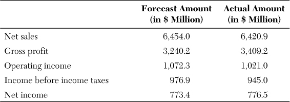
Thus, despite our simplistic assumptions, our forecast was quite realistic.
18. We can estimate this growth rate in sales using the goal seek feature in Excel. To do so, Set Cell should be linked to the cell that contains net income for 2012 (the output cell), To Value should be $768.5 million, and By Changing Cell should be linked to the cell that contains the growth rate in sales (the input cell). Excel will perform iterative calculation on the input cell until the output cell is equal to the specified value.

Appendix 2B: Preparation of a Cash Flow Statement
The demand for cash flow data has become so prevalent that most countries now require a cash flow statement. (Some countries require a cash flow statement only for publicly traded companies or for large companies.) The analyst must be prepared to develop a cash flow statement from available financial data.
Cash Flow Fundamentals
To prepare a cash flow statement, the analyst needs (1) an income statement for the current period and (2) the balance sheets at the beginning and end of the period. With only these three financial statements, the analyst can prepare an approximate cash flow statement using the four-step process outlined below. A more complete cash flow statement is possible where detailed data are given in the footnotes to the financial statements.
To begin, recall that the fundamental accounting equation for the balance sheet is given as follows:
Assets = Liabilities + Shareholders'Equity
Or:
A = L + SE
Substituting the major components of a company’s assets, liabilities, and shareholders’ equity yields:
CA + NCA = CL + NCL + CS + RE
Here, CA refers to current assets, NCA to noncurrent assets, CL to current liabilities, NCL to noncurrent liabilities, CS to capital stock, and RE to retained earnings.
Decomposing the current asset category into cash (C) and all other current assets (OCA) yields yet another version of the fundamental accounting equation:
At this juncture, it is helpful to recognize that a cash flow statement is nothing more than a formal explanation of the positive and negative changes to a company’s cash account. The cash flow statement lists where a company’s cash inflows came from and how the various cash outflows were used. Having access to a company’s internal accounting records makes preparing a cash flow statement a simple exercise; it involves merely listing the various inflows and outflows to the company’s cash account. Such access is rarely available, however. Thus, a methodology is needed so that the analyst can build a cash flow statement from available financial information.
Because a cash flow statement is a listing of the various changes in a company’s cash account, it can be expressed in its simplest form by the following equation:
Here, B is the beginning of the accounting period, E is the end of the period, and ∆ is change.
Using a few basic algebraic concepts, it is possible to redefine Equation 2B.2 in terms of Equation 2B.1. Putting the subscripts B and E on the elements of Equation 2B.1 yields:
CB + OCAB + NCAB = CLB + NCLB + CSB + REB
And:
CE + OCAE + NCAE = CLE + NCLE + CSE + REE
Isolating CB and CE on the left side of these two equations yields:
CB = CLB + NCLB + CSB + REB - OCAB - NCAB
And:
CE = CLE + NCLE + CSE + REE-OCAE-NCAE
Subtracting the first equation from the second one yields:

Both Equations 2B.2 and 2B.3 are representations of the cash flow statement, but the latter is a more explicit, formalized version than the former. More important, Equation 2B.3 provides a simple approach to the preparation of a cash flow statement; in words, it tells us that a cash flow statement can be prepared by listing the changes in all the balance sheet accounts.
From this observation, we can formulate a four-step procedure to create a basic but instructive cash flow statement:
1. Identify the change in the cash and cash equivalents account. Cash equivalents are short-term (often three months or less), virtually risk-free securities (such as debt securities issued by national or local governments). This figure represents the “bottom line” of the cash flow statement. All increases and decreases in cash must net to this figure. It is a check figure to verify the accuracy of the cash flow statement.
2. Calculate the change in all balance sheet accounts by subtracting the beginning balance from the ending balance.
3. Identify each balance sheet account with the activity category most closely related to it: operating (O), investing (I), or financing (F). As a general rule, the following associations are usually made, although exceptions exist: Changes in all other current assets, current liabilities, and retained earnings are associated with operating activities; changes in noncurrent assets are associated with investing activities; and changes in noncurrent liabilities and capital stock are associated with financing activities.
4. Place each individual balance sheet account (except cash) under one of three activity categories, and identify whether the change in the account balance involves a cash inflow or outflow. Recall that the total sources and uses of cash must aggregate to the check figure identified in step 1.
An Illustration
To illustrate the four-step process of building a cash flow statement, we consider the financial statements of Worldwide Enterprises, Inc. (WWE). Exhibit 2B.1 presents WWE’s income statement for 2012, including the split of net income between dividends and retained earnings.
Exhibit 2B.1 Worldwide Enterprises, Inc.: Income Statement for the Year Ending 31 December 2012 (in Millions)

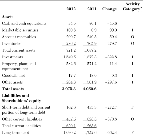
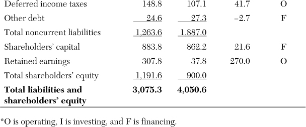
Exhibit 2B.2 presents the WWE balance sheets for 2011 and 2012, and applies the four-step procedure described previously.
1. The check figure for WWE’s cash flow statement is a decrease of 45.6 million (34.5 − 80.1). Thus, WWE’s cash outflows must have exceeded its cash inflows by 45.6 million.
2. Calculate the change in all the balance sheet accounts by subtracting the beginning (2011) balance from the ending (2012) balance; Exhibit 2B.2 shows these values in the column headed “Change.”
3. Identify the activity category associated with each balance sheet account. This is done in the last column of Exhibit 2B.2. It is important to note that judgment calls are necessary at this step. For example, even though most current liabilities, such as accounts payable and accrued liabilities payable, are typically associated with a company’s operating activities, some current liabilities (such as the current portion of long-term debt) are more correctly considered to be related to financing activities. Without specific knowledge of the transactions that gave rise to a particular account, it is difficult to be certain of an account’s proper classification. A misclassification of an account will not lead to an unbalanced cash flow statement, but it will misspecify the relative totals of the three activity categories.
4. Exhibit 2B.3 contains the preliminary cash flow statement derived from changes in the balance sheet accounts organized under the three activity categories. Remember that an increase (decrease) of an asset is a use (source) of cash, whereas an increase (decrease) of a liability is a source (use) of cash. Note that the total of the three activity categories equals the change in the cash account (a decrease of 45.6 million); this ensures that the cash flow statement was constructed correctly.
Exhibit 2B.3 Worldwide Enterprises, Inc.: Preliminary Cash Flow Statement for the Year Ending 31 December 2012 (in $ Millions)*
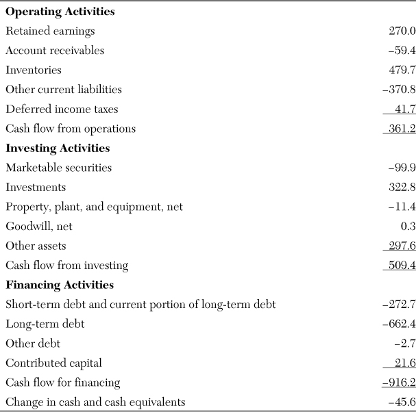
We can conclude from the preliminary cash flow statement in Exhibit 2B.3 that WWE generated cash flows from operations (CFFO) of $361.2 million and cash flows from investing (CFFI) of $509.4 million, while spending $916.2 million on financing activities (primarily retiring debt). For many financial analyses, the preliminary cash flow statement is sufficient; however, a more accurate cash flow statement is sometimes desirable. In this case, we can refine the preliminary cash flow statement using other available information. In preparing Exhibit 2B.3, only data from WWE’s balance sheet were used, but it is possible to incorporate the income statement data from Exhibit 2B.1 as well. For example, Exhibit 2B.1 reveals that, WWE’s net income was $321 million in 2012. Of this, $51 million was paid in dividends and $270 million was transferred to retained earnings. Note that this amount of $270 million is the same as the change in the retained earnings account on the balance sheet. By substituting the amount of net income and the amount of dividends to the amount of retained earnings in our preliminary cash flow statement in Exhibit 2B.3, we can produce a refined measure of the company’s cash flows. The restated figures follow:

Observe that including the additional income statement data did not change the check figure—a decrease in cash and cash equivalent of 45.6 million—but it resulted in a restatement of the CFFO and the cash flows from financing (CFFF). Our restated figures suggest that the CFFO was actually $412.2 million, instead of $361.2 million, and that the CFFF was –$967.2 million instead of –$916.2 million. This refinement did not affect the CFFI.
Another common refinement for the analyst involves depreciation and amortization. Depreciation is an accrual accounting concept in which the original cost of acquiring a depreciable asset is allocated over the many periods one is expected to benefit from the asset. Thus, the depreciation expense is the portion of an asset’s cost allocated to a given accounting period; it represents neither a current cash inflow nor a current cash outflow, but is merely an allocation of a cash expenditure made in an earlier period. Because the depreciation expense is one of the largest expense items deducted in arriving at net income, the analyst usually must adjust net income for this item, to avoid understating the actual CFFO.
Exhibits 2B.1 and 2B.2 show the depreciation expense for 2012 and the change in property, plant, and equipment, net of accumulated depreciation, respectively. Without reference to the depreciation charge of $30 million in 2012, our initial conclusion from Exhibit 2B.3 was that $11.4 million was spent on new property, plant, and equipment (PP&E) (an outflow of cash). By including the depreciation expense of $30 million, we see that the actual cash spent on new PP&E was $41.4 million. With these two figures, we can further refine our preliminary cash flow statement from Exhibit 2B.3:
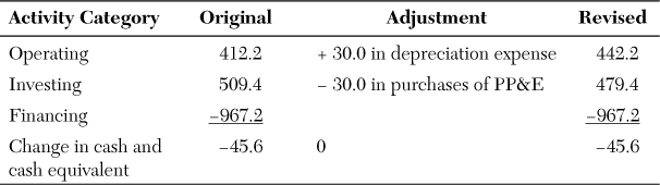
Including the depreciation expense does not change the check figure of $45.6 million, but it affects both the CFFO and the CFFI. Our restated figures suggest that the CFFO was $442.2 million instead of $412.2 million, and that the CFFI was $479.4 million instead of $509.4 million. This refinement did not affect the CFFF.
A final modification to our preliminary cash flow statement is possible by incorporating the fact that WWE’s net income of $321 million includes $75 million representing WWE’s “equity in loss of unconsolidated subsidiary.” To obtain an accurate estimate of only WWE’s CFFO, analysts frequently remove those income or loss items relating to affiliated or associated companies. In this instance, the $75 million reduction in WWE’s net income should be removed and transferred to the investing activities section as an adjustment to the investments account. This modification produces the following restated amounts:
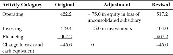
Incorporating these three modifications into Exhibit 2B.3 provides the final version of WWE’s cash flow statement, which is presented in Exhibit 2B.4.
Exhibit 2B.4 Worldwide Enterprises, Inc.: Cash Flow Statement for the Year Ending 31 December 2012 (in Millions)*
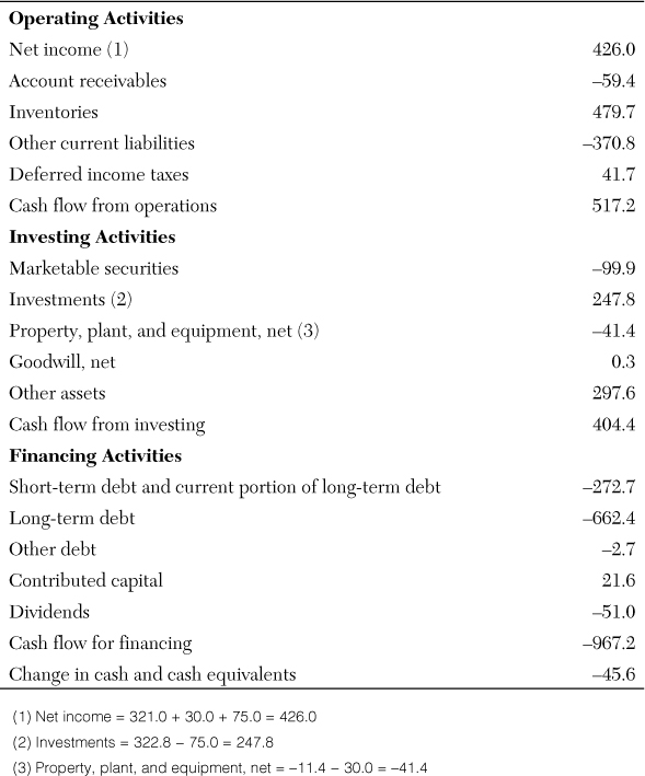
The three refinements, involving retained earnings (net income and dividends), PP&E (depreciation and purchases), and equity in the earnings of an unconsolidated subsidiary, illustrate the benefit of adjusting the preliminary cash flow statement when additional data are available. Including income statement and footnote data enables the analyst to build a more accurate cash flow statement and get better estimates of the company’s CFFO, CFFI, and CFFF.
Direct Versus Indirect Methods
Although no additional information is available for further refinement of WWE’s cash flow statement, a final consideration involves the presentation format of the operations section of the cash flow statement. Two alternative approaches exist for presenting the CFFO: the direct method and the indirect method.
Although these two approaches to formatting the operations section of the cash flow statement originated in the United States, they have gained widespread acceptance globally. Most companies that present a cash flow statement usually prefer the indirect method, which is the format Exhibit 2B.4 adopts. However, most analysts prefer the direct method because of the additional insights this format provides regarding a company’s operations.
To illustrate the construction of a direct-method version of the CFFO, we begin with the major elements of WWE’s income statement (see Exhibit 2B.1) and then adjust these elements for the various balance sheet accounts that relate to them. For example, operating revenues should be adjusted for the change in receivables, and operating expenses should be adjusted for the depreciation expense and the change in inventories, deferred income taxes, and other current liabilities.

Note that, under both the direct and indirect methods, WWE’s CFFO remains the same ($517.2 million). However, under the direct method, rearranging data enables us to identify two additional cash flow items: cash flow from operating revenues ($1,678.5 million) and cash flow for operating expenses (–$1,161.3 million). These two figures can be quite revealing about a company’s internal operations. For example, the relationship of cash operating revenues to accrual operating revenues (1,678.5/1,737.9) shows the rate at which cash is produced for each currency unit of sales—in this case, about 96.6 percent. Analysts often use this ratio to assess the quality of a company’s revenue recognition policy. In general, the higher the relationship between cash and accrual revenues, the higher the quality of a company’s revenue recognition policy. In our example, the relationship is quite strong—it approaches 100 percent. Thus, we can conclude that WWE’s revenue recognition policy is appropriate and can be relied upon in forecasts of future revenues. When the relationship is low (70 percent or less), it often indicates that the company is using an aggressive revenue recognition policy and, consequently, could be recording accrual sales in advance of receiving the cash from those sales. When this occurs, it is referred to as front-end loading and can indicate that current revenues are an inappropriate basis for forecasting future revenues.
Similarly, we can use the relationship between cash operating expenses and accrual operating expenses (1,161.3/1,341.9) to evaluate a company’s expense recognition policy. For most companies, the relationship of its cash to accrual operating expenses is less than 1, largely because of the adjustment for such noncash expenses as depreciation, amortization, and the change in deferred income taxes. However, where this relationship is substantially greater than 1, it could indicate rear-end loading. Rear-end loading occurs when a company incurs significant cash expenditures that are accounted for as assets instead of expenses. In some instances, the capitalization of such expenditures to the balance sheet is justified, whereas in others, it might not be. In any case, when the relationship of cash operating expenses to accrual operating expenses is large, most analysts see a red flag that requires further investigation.
The topics of front-end loading and rear-end loading are important due diligence considerations when the analyst reviews the accounting policies of an acquisition target. We return to these considerations in Chapter 5, “Accounting Dilemmas in Valuation Analysis.”
Summary
The purpose of this appendix was to present a simple four-step process to help analysts prepare a cash flow statement. A thorough financial analysis would be incomplete without a review of a company’s cash flows. Analysts must have the skill to prepare a pro forma cash flow statement from pro forma balance sheet and income statement data because the pro forma cash flow data is central to any target company’s valuation, as we see in Chapter 3, “Traditional Valuation Methods.”