
1. Introduction
1.1 Introduction
Every day, businesses face decision choices. For example, should a bank choose to expand organically by opening new branches, or should it expand by acquiring another bank with its own network of branches. Or, should a technology company release a new version of a product line now, and thereby cannibalize sales of its existing product line, or should it wait a year at the risk of giving its competitors time to catch up. The key to success in business is to make sound, or value-creating, business decisions. Every choice a business manager can potentially make has risk associated with it.1 In turn, every choice also has some upside, or positive return, associated with it. A sound decision is one that balances this risk and return to create value for the owners of the business, whether those are public shareholders or a private ownership group.2 However, to make value-creating business decisions, a manager needs to be able to first quantify, or measure, the risk and return inherent in each of the decision choices he is facing, and then convert these risk-return combinations into ex-ante measures of value creation. This is where the topic of valuation comes into play. Valuation is simply the conversion of risk and return into monetary value. The value could be of intangible assets like ideas or potential projects, or it could be of tangible assets like a manufacturing plant or the shares of a business. The common theme underlying valuation, however, is that it allows managers to make better business decisions by quantifying into a single metric the risk and return inherent in all business decision choices.
Every decision that a business faces can be conceptualized as a node on a decision tree, as shown in Figure 1.1. A manager facing a decision is trying to decide which of multiple paths emanating from this node he wants to take for the business. The figure illustrates the example of a manager deciding whether to build a manufacturing plant. The two possible paths are to build the plant or to not build the plant. Once the initial decision to build or not build is made, the decision tree branches off again into the capacity of the plant and again to the number of assembly lines. Each of the branches represents a set of possible outcomes that could occur. The role of valuation, then, is to quantify the value created (or destroyed) by deciding to head down a specific path. For example, the value created by building a plant with a 100,000 unit capacity containing one large assembly line would need to be quantified, as would the value created by not building a plant at all.

Note, however, that this path is only a decision path; it is not an outcome path. While a manager may decide to take a particular path, the result from taking the path is uncertain, and it might take many years before it becomes a known quantity. A more quantitative way to state this is that there is a probability distribution of possible results from the decision to take a path. Therefore, the process of valuation must take into account this probability distribution of outcomes (or risk) involved in taking a specific path.
1.2 Present Value
The standard measure that delivers the expected value created by a business decision, incorporating the full probability distribution of possible results, or payoffs, is present value. The present value of a business decision is defined mathematically as follows:
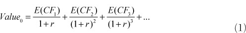
The result of evaluating the right-hand side of this equation is the value (at time 0) created by pursuing a business decision (for example, going down a specific node on the decision tree in Figure 1.1). On the right-hand side of Equation 1, E(CF1), E(CF2), and E(CF3) all denote expected cash flows in subsequent periods 1, 2, and 3 (the periods could be in months, quarters, years, and so on) due to undertaking the business decision, or project.3 Note that these are expected future cash flows. The value creation measure is evaluated at time 0, at the very start of the project. Therefore, we are evaluating what would be the value created if this project is undertaken. Because we are calculating the value of pursuing this business decision at time period 0, before the uncertainty of the project has resolved itself, we have to put in our expectations of future cash flows rather than actual, or realized, cash flows.
In the denominator of Equation 1 is the discount rate, r. The discount rate denotes the expected return that a business expects for taking on the risk associated with the project.
Equation 1 is modeling the riskiness of the project under consideration as a set of risky cash flows. These cash flows are modeled as a set of probability distributions (see Figure 1.2). The mean of each distribution is captured by the expected value of each cash flow. In Figure 1.2, the first bell-shaped curve, with a mean of E(CF1), represents the probability distribution of the cash flows in period 1, the second curve (with a mean of E(CF2)) represents the distribution of cash flows in period 2, and so on.

The variance of each distribution gives us the risk of the cash flows. In Figure 1.2, the variance is given by the “width” of the bell-shaped curve. The wider the curve, the greater the range of possible cash flows generated by the project for that period. The area under the curve shows the likelihood of a given range of cash flow outcomes. For example, the area under the first curve and between the points minus one standard deviation (–1 sd) and plus one standard deviation (1 sd) gives the likelihood that the cash flow from the project in the first period will fall within one standard deviation of the mean expected cash flow. In Equation 1, the variance, or risk, of cash flows is captured by the discount rate. The higher the risk, the higher the discount rate; that is, the more risk that a business decision entails, the higher the expected return the business expects as compensation for taking that risk (if it decides to do so).
The number of terms on the right-hand side of Equation 1 depends on the number of periods over which the business will be earning cash flows for undertaking this project. All future time periods in which the business realizes cash flows from undertaking this project, no matter how far out into the future these might be, need to be incorporated.
Although it might seem simplistic initially, this present value equation is the foundation for all of modern finance and, in particular, the topic of our book: financial valuation. Of course, the formula itself is easy to understand, but implementing it in practical business settings is the real challenge. In many ways, to do this well is an art. The goal of this book is to introduce the basics and a few advanced concepts about how to apply valuation to practical business problems that executives face.
1.3 Financial Statements and Analysis
The first step for implementing valuation is to understand exactly what we are trying to value. From a conceptual standpoint, it helps to have a couple of diagrams in mind when doing any type of valuation activity: the financial statements for the project. Figure 1.3 shows a balance sheet for a possible project that a firm is considering undertaking. For the purpose of valuation, all economic agents/quantities, whether they are companies, people, or assets (tangible or intangible), can be represented by balance sheets and income statements. We use this concept throughout this book. So, if you are unsure how to do this or find it hard to think about this conceptually, the book will provide many examples. Figure 1.3 is our first example of this. It denotes the balance sheet representation (as well as its associated income statement representation) of a project (in this case, the construction of a manufacturing plant). As with any balance sheet, the left-hand side represents the assets (in this case, the manufacturing plant), and the right-hand side represents the liabilities and the owners’, or shareholders’, equity.4 When we are doing a valuation, we are always valuing some part of this balance sheet. The income statement is a representation of the various cash flows produced by (or operating) the asset on the left-hand side of the balance sheet.
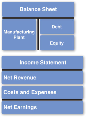
Before we do a valuation, we want to make sure that we analyze all aspects of this balance sheet and its associated income statement. This is precisely the goal of Chapter 2, “Financial Statement Analysis.” Chapter 2 discusses a few of the concepts and techniques to analyze this balance sheet and income statement. We will go through important linkages within the balance sheet, within the income statement, and across these two financial statements. We will also demonstrate some techniques to tease out what are the sensitive factors for success in these financial statements and how to figure these out. The goal of Chapter 2 is not to teach accounting; instead, we want to build on your existing foundation of knowledge in accounting to emphasize certain concepts and to introduce some new concepts that will prove particularly useful for valuation.
1.4 Financial Forecasting
The balance sheet and income statement in Figure 1.3 presents a static image of the project, as it looks at one point in time and the cash flows it produced in the time period just preceding that point in time. To conduct a valuation of a project, however, we need to figure out how a project will do over time, through the life of the project. Specifically, we need to figure out future payoffs, or cash flows, from the project if we are to use Equation 1. To do this, we need to figure out what the future balance sheets and income statements for this project will look like. So, we will have to learn how to forecast balance sheets and income statements. This is the goal of Chapter 3, “Financial Forecasting.” Chapter 3 discusses simple, but commonly used, tools and techniques for forecasting income statement and balance sheets (and, indirectly, cash flow statements). A critical element of forecasting a balance sheet is to make sure that all the expected future balance sheets balance (that is, that the asset side equals the sum of liabilities and owners’ equity). As you will discover, enforcing this constraint will give you the first critical input for Equation 1, expected future cash flows.
1.5 Free Cash Flows
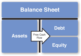
After we have constructed pro forma, or projected, financial statements for the project that we are trying to value, we can calculate the expected future cash flows, E(CF1), E(CF2), ... needed for Equation 1. To illustrate this point, Figure 1.4 presents a projected balance sheet. The cash flows that need to be input into Equation 1 are known as free cash flows and are depicted in Figure 1.4 by the arrow labeled Free Cash Flow. This diagram is conveying a picture of what precisely we are determining when we calculate free cash flows for a present value computation. For a typical project at a typical company, the left-hand side of the balance sheet represents the “business,” while the right-hand side represents the financing. Therefore, the left-hand side of the balance sheet generates the revenues and nonfinancing costs associated with the project.5 These cash flows flow from the left-hand side to the right-hand side. The right-hand side can be broken down crudely into debt and equity. Therefore, the cash flows that are being generated by the business are flowing to those entities that are financing the business: the debt holders and the equity holders. If we want to do a valuation from the perspective of all financial claimants (both debt and equity holders), the cash flows used in Equation 1 are the free cash flows. This would produce a value for the entire left-hand side of the balance sheet. Chapter 4, “Free Cash Flows,” covers this concept of free cash flows and goes into the detail about how to calculate free cash flows. The goal of Chapter 4 is to be able to produce all the numbers needed for the numerators in Equation 1 for any business project or company that one might want to value.
1.6 Discount Rates
Once the numerators in Equation 1 are calculated, all that is needed to do a valuation is to calculate the denominators in Equation 1. This is the goal of Chapter 5, “Cost of Capital.” Calculating this cost of capital (or equivalently, the required/expected rate of return)6 for a project is actually a difficult task, and one that the field of finance is still heavily researching. As a result, there is no universally agreed-upon methodology for doing these calculations.7 Chapter 5 presents a couple of the basic theories for determining the cost of capital and then also shows a couple of methods that are used in practice. Regardless of how one chooses to calculate a cost of capital, the procedure for decomposition of this value into other cost of capital values, such as cost of debt capital and cost of equity capital, is universally agreed upon, and this is what we cover next in Chapter 5. Included in this discussion is a measure called the asset cost of capital.
The discussion of these topics naturally brings up the question of how capital structure affects the expected return of the left-hand side of the balance sheet. It is at this point that we will discuss the implications of financing choices such as tax shields and costs of financial distress. As shown in Figure 1.5, these financing implications alter the value of the left-hand side of the balance sheet (and consequently the right-hand side as well), which in turn affects cost of capital calculations. Therefore, an important part of the discussion in Chapter 5 is the procedure for calculating the cost of capital taking into account the effects of capital structure decisions.

1.7 Valuation Frameworks
Chapter 6, “Putting It All Together: Valuation Frameworks,” pulls all the concepts presented in the previous chapters together and shows how to evaluate Equation 1 and determine a measure of value for a project. At the end of Chapter 5, we explain how the creation of costs and benefits due to capital structure decisions, such as tax shields, alters the value of the left-hand side of the balance sheet. This means that the cash flow effects of capital structure decisions need to be projected out so that the present value implications of these decisions can be measured. This leads to two different ways of computing the present value of a project using Equation 1, depending on how changes in the capital structure are likely to occur. We will first demonstrate the technique known as adjusted present value (APV). APV incorporates the effects of all time-varying capital structure decisions and is therefore a universal methodology for evaluating the present value of a project. However, in the special case where the debt-to-equity ratio of a project is kept constant through time, we will show that the APV approach can be simplified to another approach utilizing the weighted average cost of capital (WACC).8 The WACC-based approach allows for a much simpler and faster evaluation of Equation 1, but it can be used only under the restriction that the proportion of debt and equity on the right-hand side of the balance sheet remain the same through time (though the total amount of debt and equity may increase or decrease through time). Finally, we will introduce another special case of APV in Chapter 6 known as flow to equity (FTE). The FTE approach is widely used in the field of private equity, especially in buyout situations. We will show how to utilize FTE and how FTE evolves from APV, and we will also show FTE’s relationship to WACC.
1.8 Summary
In summary, we have organized the book according to the sequence one would generally follow in performing a valuation. Chapter 2 shows how to perform preliminary financial analysis on a potential business project. Our goal ultimately is to be able to evaluate the present value relation in Equation 1 for the project at hand. Chapter 3 starts this process by demonstrating how to calculate future financial statements for the project. Chapter 4 then shows how you take these forecasts and generate free cash flow forecasts, the numerator in Equation 1. Chapter 5 then presents several approaches for calculating a discount rate, the denominator in Equation 1, for the project. In Chapter 5, you also learn that financing choices can have value implications for any project. Chapter 6 shows how to incorporate these value implications in the evaluation of Equation 1. In Chapter 6, we also bring together the evaluation of the numerator and denominator of Equation 1 to finish the valuation. Thus, by the end of this book, you should have a solid conceptual understanding of valuation as well as a substantial amount of practical knowledge about how to go about executing a valuation of a potential business decision.
Endnotes
1. Even not making a choice has a risk (an opportunity risk of sorts).
2. This concept also applies to nonprofits, where the endowment of the nonprofit may be thought of as the shareholder that potentially accrues value.
3. It is important to distinguish subsequent periods of time versus subsequent decisions on a one-period decision tree (such as in Figure 1.1). Equation 1 contains cash flows over multiple time periods for a single decision path (with multiple decision nodes, such as in Figure 1.1) that was chosen at time 0.
4. The right side is also commonly thought of as the financing structure of the left-hand side. Therefore, in Figure 1.3, the right-hand side is composed of a set of investors who provided debt financing for the manufacturing plant and a set of investors who provided equity financing. Another common view of the right-hand side is as the ownership structure. The equity holders own the asset(s) on the left-hand side, but if equity holders cannot pay the debt holders what they are due, the debt holders will take ownership of the asset(s).
5. It is important to note here that this statement does not hold true if the project is a financial institution. For financial institutions, the “business” is on both the left- and right-hand sides of the balance sheet. For example, the business of a bank might be to take deposits and make loans. However, the deposits would be on the right-hand side of the balance sheet, while the loans are on the left-hand side. We discuss this in more detail later in the book.
6. We use the terms cost of capital, required rate of return, expected rate of return, and discount rate interchangeably throughout the book. All of these terms refer to the discount rate used to discount cash flows.
7. This is one of the reasons that we see a proliferation of investment funds in the world. If two fund managers cannot agree on the expected rate of return on, for example, a business, one may decide to buy shares in that business, while one decides to sell shares in the same business.
8. Because this approach uses WACC, it is often referred to simply as the WACC approach.