Search in book...
Toggle Font Controls
Create new playlist

Name your new playlist

Playlist description (optional)
Sign In

Email address

Password

Forgot Password?

or

Continue with Facebook

Continue with Google
Sign Up

Full Name

Email address

Confirm Email Address

Password

or

Continue with Facebook

Continue with Google

7.2 Comparing Two Population Means: Independent Sampling

In this section, we develop both large-sample and small-sample methodologies for comparing two population means. In the large-sample case, we use the z-statistic; in the small-sample case, we use the t-statistic.

Large Samples

DIETS Example 7.1 A Large-Sample Confidence Interval for (μ1−μ2) $(μ_{1} - μ_{2})$ —Comparing Mean Weight Loss for Two Diets

Problem

A dietitian has developed a diet that is low in fats, carbohydrates, and cholesterol. Although the diet was initially intended to be used by people with heart disease, the dietitian wishes to examine the effect this diet has on the weights of obese people. Two random samples of 100 obese people each are selected, and one group of 100 is placed on the low-fat diet. The other 100 are placed on a diet that contains approximately the same quantity of food, but is not as low in fats, carbohydrates, and cholesterol. For each person, the amount of weight lost (or gained) in a three-week period is recorded. The data, saved in the DIETS file, are listed in Table 7.1. Form a 95% confidence interval for the difference between the population mean weight losses for the two diets. Interpret the result.

Solution

Recall that the general form of a large-sample confidence interval for a single mean $μ$ is $\bar{x} \pm z_{α / 2} σ_{\bar{x}} .$ That is, we add and subtract $z_{α / 2}$ standard deviations of the sample estimate $\overline{x}$ to and from the value of the estimate. We employ a similar procedure to form the confidence interval for the difference between two population means.

Let $μ_{1}$ represent the mean of the conceptual population of weight losses for all obese people who could be placed on the low-fat diet. Let $μ_{2}$ be similarly defined for the other diet. We wish to form a confidence interval for $(μ_{1} - μ_{2}) .$ An intuitively appealing estimator for $(μ_{1} - μ_{2})$ is the difference between the sample means, $({\overline{x}}_{1} - {\overline{x}}_{2}) .$ Thus, we will form the confidence interval of interest with

$({\bar{x}}_{1} - {\bar{x}}_{2}) \pm z_{α / 2} σ_{({\bar{x}}_{1} - {\bar{x}}_{2})}$

Alternate View

Weight Losses for Low-Fat Diet

8 10 10 12 9 3 11 7 9 2

21 8 9 2 2 20 14 11 15 6

13 8 10 12 1 7 10 13 14 4

8 12 8 10 11 19 0 9 10 4

11 7 14 12 11 12 4 12 9 2

4 3 3 5 9 9 4 3 5 12

3 12 7 13 11 11 13 12 18 9

6 14 14 18 10 11 7 9 7 2

16 16 11 11 3 15 9 5 2 6

5 11 14 11 6 9 4 17 20 10

Weight Losses for Regular Diet

6 6 5 5 2 6 10 3 9 11

14 4 10 13 3 8 8 13 9 3

4 12 6 11 12 9 8 5 8 7

6 2 6 8 5 7 16 18 6 8

13 1 9 8 12 10 6 1 0 13

11 2 8 16 14 4 6 5 12 9

11 6 3 9 9 14 2 10 4 13

8 1 1 4 9 4 1 1 5 6

14 0 7 12 9 5 9 12 7 9

8 9 8 10 5 8 0 3 4 8

Data Set: DIETS

Assuming that the two samples are independent, we write the standard deviation of the difference between the sample means (i.e., the standard error of ${\overline{x}}_{1} - {\overline{x}}_{2}$ ) as

$σ_{({\bar{x}}_{1} - {\bar{x}}_{2})} = \sqrt{\frac{σ_{1}^{2}}{n_{1}} + \frac{σ_{2}^{2}}{n_{2}}}$

Typically (as in this example), the population variances $σ_{1}^{2}$ and $σ_{2}^{2}$ are unknown. Since the samples are both large $(n_{1} = n_{2} = 100)$ , the sample variances $s_{1}^{2}$ and $s_{2}^{2}$ will be good estimators of their respective population variances. Thus, the estimated standard error is

$σ_{({\bar{x}}_{1} - {\bar{x}}_{2})} \approx \sqrt{\frac{s_{1}^{2}}{n_{1}} + \frac{s_{2}^{2}}{n_{2}}}$

Summary statistics for the diet data are displayed at the top of the SPSS printout shown in Figure 7.1. Note that ${\overline{x}}_{1} = 9.31, {\overline{x}}_{2} = 7.40, s_{1} = 4.67,$ and $s_{2} = 4.04.$ Using these values and observing that $α = .05$ and $z_{.025} = 1.96,$ we find that the 95% confidence interval is, approximately,

$(9.31 - 7.40) \pm 1.96 \sqrt{\frac{{(4.67)}^{2}}{100} + \frac{{(4.04)}^{2}}{100}} = 1.91 \pm (1.96) (.62) = 1.91 \pm 1.22$

or (.69, 3.13). This interval (rounded) is highlighted in Figure 7.1.

Using this estimation procedure over and over again for different samples, we know that approximately 95% of the confidence intervals formed in this manner will enclose the difference in population means $(μ_{1} - μ_{2}) .$ Therefore, we are highly confident that the mean weight loss for the low-fat diet is between .69 and 3.13 pounds more than the mean weight loss for the other diet. With this information, the dietitian better understands the potential of the low-fat diet as a weight-reduction diet.

Look Back

If the confidence interval for $(μ_{1} - μ_{2})$ contains 0 [e.g., $(- 2.5, 1.3)$ ], then it is possible for the difference between the population means to be 0 (i.e., $μ_{1} - μ_{2} = 0$ ). In this case, we could not conclude that a significant difference exists between the mean weight losses for the two diets.

Now Work Exercise 7.6a

The justification for the procedure used in Example 7.1 to estimate $(μ_{1} - μ_{2})$ relies on the properties of the sampling distribution of $({\overline{x}}_{1} - {\overline{x}}_{2}) .$ The performance of the estimator in repeated sampling is pictured in Figure 7.2, and its properties are summarized in the following box:

Properties of the Sampling Distribution of $({\bar{x}}_{1} - {\bar{x}}_{2})$

The mean of the sampling distribution of $({\overline{x}}_{1} - {\overline{x}}_{2})$ is $(μ_{1} - μ_{2}) .$
If the two samples are independent, the standard deviation of the sampling distribution is

$σ_{({\bar{x}}_{1} - {\bar{x}}_{2})} = \sqrt{\frac{σ_{1}^{2}}{n_{1}} + \frac{σ_{2}^{2}}{n_{2}}}$

where $σ_{1}^{2}$ and $σ_{2}^{2}$ are the variances of the two populations being sampled and $n_{1}$ and $n_{2}$ are the respective sample sizes. We also refer to $σ_{({\bar{x}}_{1} - {\bar{x}}_{2})}$ as the standard error of the statistic $({\overline{x}}_{1} - {\overline{x}}_{2}) .$
By the Central Limit Theorem, the sampling distribution of $({\overline{x}}_{1} - {\overline{x}}_{2})$ is approximately normal for large samples.

In Example 7.1, we noted the similarity in the procedures for forming a large-sample confidence interval for one population mean and a large-sample confidence interval for the difference between two population means. When we are testing hypotheses, the procedures are again similar. The general large-sample procedures for forming confidence intervals and testing hypotheses about $(μ_{1} - μ_{2})$ are summarized in the following boxes:

Large, Independent Samples Confidence Interval for $(μ_{1} - μ_{2})$ : Normal (`z`) Statistic

$σ_{1}^{2} and σ_{2}^{2} known: ({\bar{x}}_{1} - {\bar{x}}_{2}) \pm z_{α / 2} σ_{({\bar{x}}_{1} - {\bar{x}}_{2})} = ({\bar{x}}_{1} - {\bar{x}}_{2}) \pm z_{α / 2} \sqrt{\frac{σ_{1}^{2}}{n_{1}} + \frac{σ_{2}^{2}}{n_{2}}}$

$σ_{1}^{2} and σ_{2}^{2} unknown: ({\bar{x}}_{1} - {\bar{x}}_{2}) \pm z_{α / 2} σ_{({\bar{x}}_{1} - {\bar{x}}_{2})} \approx ({\bar{x}}_{1} - {\bar{x}}_{2}) \pm z_{α / 2} \sqrt{\frac{s_{1}^{2}}{n_{1}} + \frac{s_{2}^{2}}{n_{2}}}$

Large, Independent Samples Test of Hypothesis for $(μ_{1} - μ_{2})$ : Normal (`z`) Statistic

	$σ_{1}^{2} a n d σ_{2}^{2} k n o w n$	$σ_{1}^{2} a n d σ_{2}^{2} u n k n o w n$
Test statistic:	$z_{c} = \frac{({\bar{x}}_{1} - {\bar{x}}_{2}) - D_{0}}{\sqrt{(\frac{σ_{1}^{2}}{n_{1}}) + (\frac{σ_{2}^{2}}{n_{2}})}}$	$z_{c} \approx \frac{({\bar{x}}_{1} - {\bar{x}}_{2}) - D_{0}}{\sqrt{(\frac{s_{1}^{2}}{n_{1}}) + (\frac{s_{2}^{2}}{n_{2}})}}$
	One-Tailed Tests	Two-Tailed Test
	$\begin{array}{l} H_{0} : (μ_{1} - μ_{2}) = D_{0} & H_{0} : (μ_{1} - μ_{2}) = D_{0} \end{array}$	$H_{0} : (μ_{1} - μ_{2}) = D_{0}$
	$\begin{array}{l} H_{a} : (μ_{1} - μ_{2}) < D_{0} & H_{a} : (μ_{1} - μ_{2}) > D_{0} \end{array}$	$H_{a} : (μ_{1} - μ_{2}) \neq D_{0}$
Rejection region:	$\begin{array}{l} z_{c} < - z_{α} & z_{c} > z_{α} \end{array}$	$\| z_{c} \| > z_{α / 2}$
p-value:	$\begin{array}{l} P (z < z_{c}) & P (z > z_{c}) \end{array}$	$2 P (z > z_{c}) if z_{c} is positive$
		$2 P (z < z_{c}) if z_{c} is positive$
Decision: Reject $H_{0}$ if $α > p -value$ or if test statistic $(z_{c})$ falls in rejection region where $P (z > z_{α}) = α$ , $P (z > z_{α / 2}) = α / 2,$ and $α = P (Type I error) = P (Reject H_{0} \| H_{0} true)$ . [Note: The symbol for the numerical value assigned to the difference $(μ_{1} - μ_{2})$ under the null hypothesis is $D_{0}$ . For testing equal population means, $D_{0} = 0$ .]

Conditions Required for Valid Large-Sample Inferences about $(μ_{1} - μ_{2})$

The two samples are randomly selected in an independent manner from the two target populations.
The sample sizes, $n_{1}$ and $n_{2},$ are both large (i.e., $n_{1} \geq 30$ and $n_{2} \geq 30$ ). (By the Central Limit Theorem, this condition guarantees that the sampling distribution of $({\overline{x}}_{1} - {\overline{x}}_{2})$ will be approximately normal, regardless of the shapes of the underlying probability distributions of the populations. Also, $s_{1}^{2}$ and $s_{2}^{2}$ will provide good approximations to $σ_{1}^{2}$ and $σ_{2}^{2}$ when both samples are large.)

DIETS Example 7.2 A Large-Sample Test for $(μ_{1} - μ_{2})$ —Comparing Mean Weight Loss for Two Diets

Problem

Refer to the study of obese people on a low-fat diet and a regular diet presented in Example 7.1. Another way to compare the mean weight losses for the two different diets is to conduct a test of hypothesis. Suppose we want to determine if the low-fat diet is more effective than the regular diet. Use the information on the SPSS printout shown in Figure 7.1 to conduct the test at $α = .05 .$

Solution

Again, we let $μ_{1}$ and $μ_{2}$ represent the population mean weight losses of obese people on the low-fat diet and regular diet, respectively. If the low-fat diet is more effective in reducing the weights of obese people, then the mean weight loss for the low-fat diet, $μ_{1}$ , will exceed the mean weight loss for the regular diet, $μ_{2}$ . That is $μ_{1} > μ_{2}$ .

Thus, the elements of the test are as follows:

$\begin{array}{l} H_{0} : (μ_{1} - μ_{2}) = 0 (i . e ., μ_{1} = μ_{2}; note that D_{0} = 0 for this hypothesis test) \\ H_{a} : (μ_{1} - μ_{2}) > 0 (i . e ., μ_{1} > μ_{2}) \end{array}$

$\begin{array}{l} T e s t s t a t i s t i c : z = \frac{({\bar{x}}_{1} - {\bar{x}}_{2}) - D_{0}}{σ_{({\bar{x}}_{1} - {\bar{x}}_{2})}} = \frac{{\bar{x}}_{1} - {\bar{x}}_{2} - 0}{σ_{({\bar{x}}_{1} - {\bar{x}}_{2})}} \\ R e j e c t i o n r e g i o n : z > z_{.05} = 1.645 \end{array}$

(see Figure 7.3)

Substituting the summary statistics given in Figure 7.1 into the test statistic, we obtain

$z = \frac{({\bar{x}}_{1} - {\bar{x}}_{2}) - 0}{σ_{({\bar{x}}_{1} - {\bar{x}}_{2})}} = \frac{9.31 - 7.40}{\sqrt{\frac{σ_{1}^{2}}{n_{1}} + \frac{σ_{2}^{2}}{n_{2}}}}$

Now, since $σ_{1}^{2}$ and $σ_{2}^{2}$ are unknown, we approximate the test statistic value as follows:

$\begin{matrix} z \approx \frac{9.31 - 7.40}{\sqrt{\frac{s_{1}^{2}}{n_{1}} + \frac{s_{2}^{2}}{n_{2}}}} = \frac{1.91}{\sqrt{\frac{{(4.67)}^{2}}{100} + \frac{{(4.04)}^{2}}{100}}} = \frac{1.91}{.617} = 3.09 \end{matrix}$

Figure 7.3

Rejection region for Example 7.2

[Note: The value of the test statistic is highlighted in the SPSS printout of Figure 7.1.]

As you can see in Figure 7.3, the calculated z-value clearly falls into the rejection region. Therefore, the samples provide sufficient evidence, at $α = .05,$ for the dietitian to conclude that the mean weight losses for the two diets differ.

Look Back

First, note that this conclusion agrees with the inference drawn from the 95% confidence interval in Example 7.1. However, the confidence interval provides more information on the mean weight losses. From the hypothesis test, we know only that the two means differ; that is, $μ_{1} > μ_{2} .$ From the confidence interval in Example 7.1, we found that the mean weight loss $μ_{1}$ of the low-fat diet was between .69 and 3.13 pounds more than the mean weight loss $μ_{2}$ of the regular diet. In other words, the test tells us that the means differ, but the confidence interval tells us how large the difference is.

Second, a one-tailed hypothesis test and a confidence interval (which is two-tailed) may not always agree. However, a two-tailed hypothesis test and a confidence interval will always give the same inference about the target parameter for the same value of $α$ .

DIETS Example 7.3 The `p`-Value for a Test of $(μ - μ_{2})$

Problem

Find the observed significance level for the test in Example 7.2. Interpret the result.

Solution

The alternative hypothesis in Example 7.2, $H_{a} : μ_{1} - μ_{2} > 0,$ required an upper one-tailed test using

$z = \frac{{\bar{x}}_{1} - {\bar{x}}_{2}}{σ_{({\bar{x}}_{1} - {\bar{x}}_{2})}}$

as a test statistic. Since the z-value calculated from the sample data was 3.09, the observed significance level (p-value) for the one-tailed test is the probability of observing a value of z at least as contradictory to the null hypothesis as $z = 3.09;$ that is,

$p -value = P (z \geq 3.09)$

This probability is computed under the assumption that $H_{0}$ is true and is equal to the highlighted area shown in Figure 7.4.

Figure 7.4

The observed significance level for Example 7.2

The tabulated area corresponding to $z = 3.09$ in Table II of Appendix B is .4990. Therefore, the observed significance level for the test is

$p -value = P (z \geq 3.09) = .5 - .4990 = .0010$

Since our selected $α$ value, .05, exceeds this p-value, we have sufficient evidence to reject $H_{0} : (μ_{1} - μ_{2}) = 0$ in favor of $H_{a} : (μ_{1} - μ_{2}) > 0$ .

Look Back

The p-value of the test is more easily obtained from a statistical software package. A MINITAB printout for the hypothesis test is displayed in Figure 7.5. The one-tailed p-value, highlighted on the printout is .001. This value agrees with our calculated p-value.

MINITAB Printout for One-Tailed Test, Example 7.3

Now Work Exercise 7.6b

Small Samples

In comparing two population means with small samples (say, either $n_{1} < 30$ or $n_{2} < 30$ or both), the methodology of the previous three examples is invalid. The reason? When the sample sizes are small, estimates of $σ_{1}^{2}$ and $σ_{2}^{2}$ are unreliable and the Central Limit Theorem (which guarantees that the z statistic is normal) can no longer be applied. But as in the case of a single mean (Section 6.5), we use the familiar Student’s t-distribution.

To use the t-distribution, both sampled populations must be approximately normally distributed with equal population variances, and the random samples must be selected independently of each other. The assumptions of normality and equal variances imply relative frequency distributions for the populations that would appear as shown in Figure 7.6.

Assumptions for the two-sample t: (1) normal populations; (2) equal variances

Since we assume that the two populations have equal variances $(σ_{1}^{2} = σ_{2}^{2} = σ^{2}),$ it is reasonable to use the information contained in both samples to construct a pooled sample estimator $σ^{2}$ for use in confidence intervals and test statistics. Thus, if $s_{1}^{2}$ and $s_{2}^{2}$ are the two sample variances (each estimating the variance $σ^{2}$ common to both populations), the pooled estimator of $σ^{2},$ denoted as $s_{p}^{2},$ is

$s_{p}^{2} = \frac{(n_{1} - 1) s_{1}^{2} + (n_{2} - 1) s_{2}^{2}}{(n_{1} - 1) + (n_{2} - 1)} = \frac{(n_{1} - 1) s_{1}^{2} + (n_{2} - 1) s_{2}^{2}}{n_{1} + n_{2} - 2}$

$s_{p}^{2} = \frac{\overset{From sample 1}{\overset{︷}{\sum {(x_{1} - {\bar{x}}_{1})}^{2} +}} \overset{From sample 2}{\overset{︷}{\sum {(x_{2} - {\bar{x}}_{2})}^{2}}}}{n_{1} + n_{2} - 2}$

where $x_{1}$ represents a measurement from sample 1 and $x_{2}$ represents a measurement from sample 2. Recall that the term degrees of freedom was is defined in Section 5.3 as 1 less than the sample size. Thus, in this case, we have $(n_{1} - 1)$ degrees of freedom for sample 1 and $(n_{2} - 1)$ degrees of freedom for sample 2. Since we are pooling the information on $σ^{2}$ obtained from both samples, the number of degrees of freedom associated with the pooled variance $s_{p}^{2}$ is equal to the sum of the numbers of degrees of freedom for the two samples, namely, the denominator of $s_{p}^{2};$ that is, $(n_{1} - 1) + (n_{2} - 1) = n_{1} + n_{2} - 2.$

Note that the second formula given for $s_{p}^{2}$ shows that the pooled variance is simply a weighted average of the two sample variances $s_{1}^{2}$ and $s_{2}^{2} .$ The weight given each variance is proportional to its number of degrees of freedom. If the two variances have the same number of degrees of freedom (i.e., if the sample sizes are equal), then the pooled variance is a simple average of the two sample variances. The result is an average, or “pooled,” variance that is a better estimate of $σ^{2}$ than either $s_{1}^{2}$ or $s_{2}^{2}$ alone.

Biography Bradley Efron (1938–present)

The Bootstrap Method

Bradley Efron was raised in St. Paul, Minnesota, the son of a truck driver who was the amateur statistician for his bowling and baseball leagues. Efron received a B.S. in mathematics from the California Institute of Technology in 1960 but, by his own admission, had no talent for modern abstract math. His interest in the science of statistics developed after he read a book by Harold Cramer from cover to cover. Efron went to Stanford University to study statistics, and he earned his Ph.D there in 1964. He has been a faculty member in Stanford’s Department of Statistics since 1966. Over his career, Efron has received numerous awards and prizes for his contributions to modern statistics, including the MacArthur Prize Fellow (1983), the American Statistical Association Wilks Medal (1990), and the Parzen Prize for Statistical Innovation (1998). In 1979, Efron invented a method—called the bootstrap—of estimating and testing population parameters in situations in which either the sampling distribution is unknown or the assumptions are violated. The method involves repeatedly taking samples of size n (with replacement) from the original sample and calculating the value of the point estimate. Efron showed that the sampling distribution of the estimator is simply the frequency distribution of the bootstrap estimates.

Both the confidence interval and the test-of-hypothesis procedures for comparing two population means with small samples are summarized in the following boxes:

Small, Independent Samples Confidence Interval for $(μ_{1} - μ_{2})$ Student’s `t`-Statistic

$({\bar{x}}_{1} - {\bar{x}}_{2}) \pm t_{α / 2} \sqrt{s_{p}^{2} (\frac{1}{n_{1}} + \frac{1}{n_{2}})}$

where $s_{p}^{2} = \frac{(n_{1} - 1) s_{1}^{2} + (n_{2} - 1) s_{2}^{2}}{n_{1} + n_{2} - 2}$

and $t_{α / 2}$ is based on $(n_{1} + n_{2} - 2)$ degrees of freedom.

[Note: $s_{p}^{2} = \frac{s_{1}^{2} + s_{2}^{2}}{2} when n_{1} = n_{2}$ ]

Small, Independent Samples Test of Hypothesis for $(μ_{1} - μ_{2})$ Student’s `t`-Statistic

$\begin{array}{r} Test statistic: & t_{c} = \frac{({\bar{x}}_{1} - {\bar{x}}_{2}) - D_{0}}{\sqrt{s_{p}^{2} (\frac{1}{n_{1}} + \frac{1}{n_{2}})}} & where s_{p}^{2} = \frac{(n_{1} - 1) s_{1}^{2} + (n_{2} - 1) s_{2}^{2}}{(n_{1} + n_{2} - 2)} \end{array}$

	One-Tailed Tests	Two-Tailed Test
	$\begin{array}{l} H_{0} : (μ_{1} - μ_{2}) & = & D_{0} & H_{0} : (μ_{1} - μ_{2}) & = & D_{0} \\ H_{a} : (μ_{1} - μ_{2}) & < & D_{0} & H_{a} : (μ_{1} - μ_{2}) & < & D_{0} \end{array}$	$\begin{matrix} H_{0} : (μ_{1} - μ_{2}) = D_{0} \\ H_{a} : (μ_{1} - μ_{2}) \neq D_{0} \end{matrix}$
Rejection region:	$\begin{array}{l} t_{c} & < & - t_{α} & t_{c} & > & t_{α} \end{array}$	$\begin{array}{l} \| t_{c} \| > t_{α / 2} \end{array}$
p-value:	$\begin{array}{l} P (t & < & t_{c}) & P (t & > & t_{c}) \end{array}$	$\begin{array}{l} 2 P (t > t_{c}) if t_{c} is positive \\ 2 P (t < t_{c}) if t_{c} is negative \end{array}$

Decision: Reject $H_{0}$ if $α > p -value$ or if test statistic $(t_{c})$ falls in rejection region where $P (t > z_{α}) = α$ , $P (t > t_{α / 2}) = α / 2,$ the distribution of t is based on $n_{d} - 1$ df, and $α = P (Type I error) = P (Reject H_{0} | H_{0} true)$ .

[Note: The symbol for the numerical value assigned to the difference $(μ_{1} - μ_{2})$ under the null hypothesis is $D_{0}$ . For testing equal population means, $D_{0} = 0$ .]

Conditions Required for Valid Small-Sample Inferences about $(μ_{1} - μ_{2})$

The two samples are randomly selected in an independent manner from the two target populations.
Both sampled populations have distributions that are approximately normal.
The population variances are equal (i.e., $σ_{1}^{2} = σ_{2}^{2}$ ).

READING Example 7.4 A Small-Sample Confidence Interval for $(μ_{1} - μ_{2})$ —Comparing Two Methods of Teaching

Problem

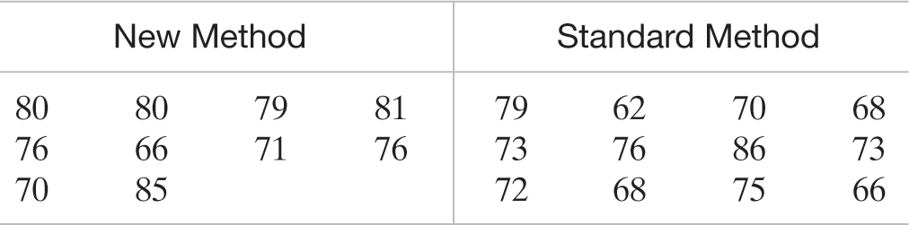
Suppose you wish to compare a new method of teaching reading to “slow learners” with the current standard method. You decide to base your comparison on the results of a reading test given at the end of a learning period of six months. Of a random sample of 22 “slow learners,” 10 are taught by the new method and 12 are taught by the standard method. All 22 children are taught by qualified instructors under similar conditions for the designated six-month period. The results of the reading test at the end of this period are given in Table 7.2.

Table 7.2 Reading Test Scores for Slow Learners

Alternate View

New Method Standard Method

80 80 79 81 79 62 70 68

76 66 71 76 73 76 86 73

70 85 72 68 75 66

Data Set: READING
1. Use the data in the table to estimate the true mean difference between the test scores for the new method and the standard method. Use a 95% confidence interval.
2. Interpret the interval you found in part a.
3. What assumptions must be made in order that the estimate be valid? Are they reasonably satisfied?

New Method	Standard Method
80	80	79	81	79	62	70	68
76	66	71	76	73	76	86	73
70	85			72	68	75	66

Solution

For this experiment, let $μ_{1}$ and $μ_{2}$ represent the mean reading test scores of “slow learners” taught with the new and standard methods, respectively. Then the objective is to obtain a 95% confidence interval for $(μ_{1} - μ_{2}) .$

The first step in constructing the confidence interval is to obtain summary statistics (e.g., $\overline{x}$ and s) on reading test scores for each method. The data of Table 7.2 were entered into a computer, and SAS was used to obtain these descriptive statistics. The SAS printout appears in Figure 7.7. Note that ${\overline{x}}_{1} = 76.4, s_{1} = 5.8348, {\overline{x}}_{2} = 72.333,$ and $s_{2} = 6.3437.$

Figure 7.7

SAS printout for Example 7.4

Next, we calculate the pooled estimate of variance to obtain

$\begin{array}{l} \begin{matrix} s_{p}^{2} \end{matrix} & = & \frac{(n_{1} - 1) s_{1}^{2} + (n_{2} - 1) s_{2}^{2}}{n_{1} + n_{2} - 2} \\ = & \begin{matrix} \frac{(10 - 1) {(5.8348)}^{2} + (12 - 1) {(6.3437)}^{2}}{10 + 12 - 2} = 37.45 \end{matrix} \end{array}$

where $s_{p}^{2}$ is based on $(n_{1} + n_{2} - 2) = (10 + 12 - 2) = 20$ degrees of freedom. Also, we find $t_{α / 2} = t_{.025} = 2.086$ (based on 20 degrees of freedom) from Table III of Appendix B.

Finally, the 95% confidence interval for $(μ_{1} - μ_{2}),$ the difference between mean test scores for the two methods, is

$\begin{array}{l} ({\bar{x}}_{1} - {\bar{x}}_{2}) \pm t_{α / 2} \sqrt{s_{p}^{2} (\frac{1}{n_{1}} + \frac{1}{n_{2}})} & = & (76.4 - 72.33) \pm t_{.025} \sqrt{37.45 (\frac{1}{10} + \frac{1}{12})} \\ = & 4.07 \pm (2.086) (2.62) \\ = & 4.07 \pm 5.47 \end{array}$

or $(- 1.4, 9.54) .$ This interval agrees (except for rounding) with the one shown at the bottom of the SAS printout of Figure 7.7.
The interval can be interpreted as follows: With a confidence coefficient equal to .95, we estimate that the difference in mean test scores between using the new method of teaching and using the standard method falls into the interval from $- 1.4$ to 9.54. In other words, we estimate (with 95% confidence) the mean test score for the new method to be anywhere from 1.4 points less than, to 9.54 points more than, the mean test score for the standard method. Although the sample means seem to suggest that the new method is associated with a higher mean test score, there is insufficient evidence to indicate that $(μ_{1} - μ_{2})$ differs from 0 because the interval includes 0 as a possible value for $(μ_{1} - μ_{2}) .$ To demonstrate a difference in mean test scores (if it exists), you could increase the sample size and thereby narrow the width of the confidence interval for $(μ_{1} - μ_{2}) .$ Alternatively, you can design the experiment differently. This possibility is discussed in the next section.
To use the small-sample confidence interval properly, the following assumptions must be satisfied:
1. The samples are randomly and independently selected from the populations of “slow learners” taught by the new method and the standard method.
2. The test scores are normally distributed for both teaching methods.
3. The variance of the test scores is the same for the two populations; that is, $σ_{1}^{2} = σ_{2}^{2} .$

On the basis of the information provided about the sampling procedure in the description of the problem, the first assumption is satisfied. To check the plausibility of the remaining two assumptions, we resort to graphical methods. Figure 7.8 is a MINITAB printout that gives normal probability plots for the test scores of the two samples of “slow learners.” The near straight-line trends on both plots indicate that the distributions of the scores are approximately mound shaped and symmetric. Consequently, each sample data set appears to come from a population that is approximately normal.

One way to check the third assumption is to examine box plots of the sample data. Figure 7.9 is a MINITAB printout that shows side-by-side vertical box plots of the test scores in the two samples. Recall from Section 2.7 that the box plot represents the “spread” of a data set. The two box plots appear to have about the same spread; thus, the samples appear to come from populations with approximately the same variance.

MINITAB normal probability plots for Example 7.4

Look Back

All three assumptions, then, appear to be reasonably satisfied for this application of the small-sample confidence interval.

Now Work Exercise 7.9

The two-sample t-statistic is a powerful tool for comparing population means when the assumptions are satisfied. It has also been shown to retain its usefulness when the sampled populations are only approximately normally distributed. And when the sample sizes are equal, the assumption of equal population variances can be relaxed. That is, if $n_{1} = n_{2},$ then $σ_{1}^{2}$ and $σ_{2}^{2}$ can be quite different, and the test statistic will still possess, approximately, a Student’s t-distribution. In the case where $σ_{1}^{2} \neq σ_{2}^{2}$ and $n_{1} \neq n_{2},$ an approximate small-sample confidence interval or test can be obtained by modifying the number of degrees of freedom associated with the t-distribution.

The next box gives the approximate small-sample procedures to use when the assumption of equal variances is violated. The test for the case of “unequal sample sizes” is based on Satterthwaite’s (1946) approximation.

Approximate Small-Sample Procedures when $σ_{1}^{2} \neq σ_{2}^{2}$

Equal Sample Sizes $(n_{1} = n_{2} = n)$

$\begin{array}{l} C o n f i d e n c e i n t e r v a l : & ({\bar{x}}_{1} - {\bar{x}}_{2}) \pm t_{α / 2} \sqrt{(s_{1}^{2} + s_{2}^{2}) / n} \end{array}$
$\begin{array}{l} T e s t s t a t i s t i c f o r H_{0} : (μ_{1} - μ_{2}) = 0 : & t = ({\bar{x}}_{1} - {\bar{x}}_{2}) / \sqrt{(s_{1}^{2} + s_{2}^{2}) / n} \end{array}$
where t is based on $ν = n_{1} + n_{2} - 2 = 2 (n - 1)$ degrees of freedom.
Unequal Sample Sizes $(n_{1} \neq n_{2})$

$\begin{array}{l} C o n f i d e n c e i n t e r v a l : & ({\bar{x}}_{1} - {\bar{x}}_{2}) \pm t_{α / 2} \sqrt{(s_{1}^{2} / n_{1}) + (s_{2}^{2} / n_{2})} \end{array}$
$\begin{array}{l} T e s t s t a t i s t i c f o r H_{0} : (μ_{1} - μ_{2}) = 0 : & t = ({\bar{x}}_{1} - {\bar{x}}_{2}) / \sqrt{(s_{1}^{2} / n_{1}) + (s_{2}^{2} / n_{2})} \end{array}$
where t is based on degrees of freedom equal to

$v = \frac{{(s_{1}^{2} / n_{1} + s_{2}^{2} / n_{2})}^{2}}{\frac{{(s_{1}^{2} / n_{1})}^{2}}{n_{1} - 1} + \frac{{(s_{2}^{2} / n_{2})}^{2}}{n_{2} - 1}}$

Note: The value of $ν$ will generally not be an integer. Round $ν$ down to the nearest integer to use the t-table.

When the assumptions are not clearly satisfied, you can select larger samples from the populations or you can use other available statistical tests called nonparametric statistical tests.

What Should You Do If the Assumptions Are Not Satisfied?

Answer: If you are concerned that the assumptions are not satisfied, use the nonparametric Wilcoxon rank sum test for independent samples to test for a shift in population distributions. (See optional Section 7.5).

Statistics in Action Revisited

Comparing Mean Price Changes

Refer to the ZixIt v. Visa court case described in the Statistics in Action (p. 368). Recall that a Visa executive wrote e-mails and made Web site postings in an effort to undermine a new online credit card processing system developed by ZixIt. ZixIt sued Visa for libel, asking for $699 million in damages. An expert statistician, hired by the defendants (Visa), performed an “event study” in which he matched the Visa executive’s e-mail postings with movement of ZixIt’s stock price the next business day. The data were collected daily from September 1 to December 30, 1999 (an 83-day period) and are available in the ZIXITVISA file. In addition to daily closing price (dollars) of ZixIt stock, the file contains a variable for whether the Visa executive posted an e-mail and the change in price of the stock the following business day. During the 83-day period, the executive posted e-mails on 43 days and had no postings on 40 days.

If the daily posting by the Visa executive had a negative impact on ZixIt stock, then the average price change following nonposting days should exceed the average price change following posting days. Consequently, one way to analyze the data is to conduct a comparison of two population means through either a confidence interval or a test of hypothesis. Here, we let $μ_{1}$ represent the mean price change of ZixIt stock following all nonposting days and $μ_{2}$ represent the mean price change of ZixIt stock following posting days. If, in fact, the charges made by ZixIt are true, then $μ_{1}$ will exceed $μ_{2}$ . However, if the data do not support ZixIt’s claim, then we will not be able to reject the null hypothesis $H_{0} : (μ_{1} - μ_{2}) = 0$ in favor of $H_{a} : (μ_{1} - μ_{2}) > 0.$ Similarly, if a confidence interval for $(μ_{1} - μ_{2})$ contains the value 0, then there will be no evidence to support ZixIt’s claim.

MINITAB comparison of two price change means

MINITAB comparison of two trading volume means

Because both sample size ( $n_{1} = 40$ and $n_{2} = 43$ ) are large, we can apply the large-sample z-test or large-sample confidence interval procedure for independent samples. A MINITAB printout for this analysis is shown in Figure SIA7.1. Both the 95% confidence interval and p-value for a two-tailed test of hypothesis are highlighted on the printout. Note that the 95% confidence interval, $(- $ 1.47, $ 1.09)$ , includes the value $0, and the p-value for the two-tailed hypothesis test (.770) implies that the two population means are not significantly different. Also, interestingly, the sample mean price change after posting days $({\bar{x}}_{1} = $ .06)$ is small and positive, while the sample mean price change after nonposting days $({\bar{x}}_{2} = - $ .13)$ is small and negative, totally contradicting ZixIt’s claim.

The statistical expert for the defense presented these results to the jury, arguing that the “average price change following posting days is small and similar to the average price change following nonposting days’ and “the difference in the means is not statistically significant.”

Note: The statistician also compared the mean ZixIt trading volume (number of ZixIt stock shares traded) after posting days to the mean trading volume after nonposting days. These results are shown in Figure SIA7.2. You can see that the 95% confidence interval for the difference in mean trading volume (highlighted) includes 0, and the p-value for a two-tailed test of hypothesis for a difference in means (also highlighted) is not statistically significant. These results were also presented to the jury in defense of Visa.

Data Set: ZIXITVISA

Exercises 7.1–7.28

Understanding the Principles

7.1 Describe the sampling distribution of $({\overline{x}}_{1} - {\overline{x}}_{2})$ when the samples are large.
7.2 To use the t-statistic to test for a difference between the means of two populations, what assumptions must be made about the two populations? About the two samples?
7.3 Two populations are described in each of the cases that follow. In which cases would it be appropriate to apply the small-sample t-test to investigate the difference between the population means?
1. Population 1: Normal distribution with variance $σ_{1}^{2}$ Population 2: Skewed to the right with variance $σ_{2}^{2} = σ_{1}^{2}$
2. Population 1: Normal distribution with variance $σ_{1}^{2}$ Population 2: Normal distribution with variance $σ_{2}^{2} \neq σ_{1}^{2}$
3. Population 1: Skewed to the left with variance $σ_{1}^{2}$
  
  Population 2: Skewed to the left with variance $σ_{2}^{2} = σ_{1}^{2}$
4. Population 1: Normal distribution with variance $σ_{1}^{2}$
  
  Population 2: Normal distribution with variance $σ_{2}^{2} = σ_{1}^{2}$
5. Population 1: Uniform distribution with variance $σ_{1}^{2}$
  
  Population 2: Uniform distribution with variance $σ_{2}^{2} = σ_{1}^{2}$
7.4 A confidence interval for $(μ_{1} - μ_{2})$ is $(- 10, 4) .$ Which of the following inferences is correct?
1. $μ_{1} > μ_{2}$
2. $μ_{1} < μ_{2}$
3. $μ_{1} = μ_{2}$
4. no significant difference between means
7.5 A confidence interval for $(μ_{1} - μ_{2})$ is $(- 10, - 4) .$ Which of the following inferences is correct?
1. $μ_{1} > μ_{2}$
2. $μ_{1} < μ_{2}$
3. $μ_{1} = μ_{2}$
4. no significant difference between means

Learning the Mechanics

7.6 In order to compare the means of two populations, independent random samples of 400 observations are selected from each population, with the following results:

Sample 1	Sample 2
${\overline{x}}_{1} = 5, 275$	${\overline{x}}_{2} = 5, 240$
$s_{1} = 150$	$s_{2} = 200$

Use a 95% confidence interval to estimate the difference between the population means $(μ_{1} - μ_{2}) .$ Interpret the confidence interval.
Test the null hypothesis $H_{0} : (μ_{1} - μ_{2}) = 0$ versus the alternative hypothesis $H_{a} : (μ_{1} - μ_{2}) \neq 0.$ Give the p-value of the test, and interpret the result.
Suppose the test in part b were conducted with the alternative hypothesis $H_{a} : (μ_{1} - μ_{2}) > 0.$ How would your answer to part b change?
Test the null hypothesis $H_{0} : (μ_{1} - μ_{2}) = 25$ versus the alternative $H_{a} : (μ_{1} - μ_{2}) \neq 25.$ Give the p-value, and interpret the result. Compare your answer with that obtained from the test conducted in part b.
What assumptions are necessary to ensure the validity of the inferential procedures applied in parts a–d?

7.7 Independent random samples of 100 observations each are chosen from two normal populations with the following means and standard deviations:

Population 1	Population 2
$μ_{1} = 14$	$μ_{2} = 10$
$σ_{1} = 4$	$σ_{2} = 3$

Let ${\overline{x}}_{1}$ and ${\overline{x}}_{2}$ denote the two sample means.

Give the mean and standard deviation of the sampling distribution of ${\overline{x}}_{1} .$
Give the mean and standard deviation of the sampling distribution of ${\overline{x}}_{2} .$
Suppose you were to calculate the difference $({\overline{x}}_{1} - {\overline{x}}_{2})$ between the sample means. Find the mean and standard deviation of the sampling distribution of $({\overline{x}}_{1} - {\overline{x}}_{2}) .$
Will the statistic $({\overline{x}}_{1} - {\overline{x}}_{2})$ be normally distributed? Explain.

7.8 Assume that $σ_{1}^{2} = σ_{2}^{2} = σ^{2} .$ Calculate the pooled estimator of $σ^{2}$ for each of the following cases:
1. $s_{1}^{2} = 200, s_{2}^{2} = 180, n_{1} = n_{2} = 25$
2. $s_{1}^{2} = 25, s_{2}^{2} = 40, n_{1} = 20, n_{2} = 10$
3. $s_{1}^{2} = .20, s_{2}^{2} = .30, n_{1} = 8, n_{2} = 12$
4. $s_{1}^{2} = 2, 500, s_{2}^{2} = 1, 800, n_{1} = 16, n_{2} = 17$
5. Note that the pooled estimate is a weighted average of the sample variances. To which of the variances does the pooled estimate fall nearer in each of cases a–d?
L07009 7.9 Independent random samples from normal populations produced the following results:

Sample 1 Sample 2

1.2 4.2

3.1 2.7

1.7 3.6

2.8 3.9

3.0
1. Calculate the pooled estimate of $σ^{2} .$
2. Do the data provide sufficient evidence to indicate that $μ_{2} > μ_{1} ?$ Test, using $α = .10 .$
3. Find a 90% confidence interval for $(μ_{1} - μ_{2}) .$
4. Which of the two inferential procedures, the test of hypothesis in part b or the confidence interval in part c, provides more information about $(μ_{1} - μ_{2}) ?$
7.10 Two independent random samples have been selected, 100 observations from population 1 and 100 from population 2. Sample means ${\overline{x}}_{1} = 70$ and ${\overline{x}}_{2} = 50$ were obtained. From previous experience with these populations, it is known that the variances are $σ_{1}^{2} = 100$ and $σ_{2}^{2} = 64.$
1. Find $σ_{({\bar{x}}_{1} - {\bar{x}}_{2})} .$
2. Sketch the approximate sampling distribution $({\overline{x}}_{1} - {\overline{x}}_{2}),$ assuming that $(μ_{1} - μ_{2}) = 5.$
3. Locate the observed value of $({\overline{x}}_{1} - {\overline{x}}_{2})$ on the graph you drew in part b. Does it appear that this value contradicts the null hypothesis $H_{0} : (μ_{1} - μ_{2}) = 5 ?$
4. Use the z-table to determine the rejection region for the test of $H_{0} : (μ_{1} - μ_{2}) = 5$ against $H_{a} : (μ_{1} - μ_{2}) \neq 5.$ Use $α = .05 .$
5. Conduct the hypothesis test of part d and interpret your result.
6. Construct a 95% confidence interval for $(μ_{1} - μ_{2}) .$ Interpret the interval.
7. Which inference provides more information about the value of $(μ_{1} - μ_{2}),$ the test of hypothesis in part e or the confidence interval in part f?

Sample 1	Sample 2
1.2	4.2
3.1	2.7
1.7	3.6
2.8	3.9
3.0

Applying the Concepts—Basic

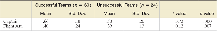
7.11 Shared leadership in airplane crews. Human Factors (Mar. 2014) published a study that examined the effect of shared leadership by the cockpit and cabin crews of a commercial airplane. Simulated flights were taken by 84 six-person crews, where each crew consisted of a two-person cockpit (captain and first officer) and a four-person cabin team (three flight attendants and a purser). During the simulation, smoke appeared in the cabin and the reactions of the crew were monitored for teamwork. Each crew was rated as working either successfully or unsuccessfully as a team. Also, each individual member was evaluated for leadership (measured as number of leadership functions exhibited per minute). The mean leadership values for successful and unsuccessful teams were compared. A summary of the test results for both captains and lead flight attendants is displayed in the table at the top of the page.

Alternate View

Successful Teams $(n = 60)$ Unsuccessful Teams $(n = 24)$

Mean Std. Dev. Mean Std. Dev. `t`-value `p`-value

Captain .66 .10 .50 .20 3.72 .000

Flight Att. .40 .24 .39 .13 0.12 .907

Source: Bienefeld, N., & Grote, G. “Shared leadership in multiteam systems: How cockpit and cabin crews lead each other to safety.” Human Factors, Vol. 65, No. 2, Mar. 2014 (Table 2).

	Successful Teams $(n = 60)$	Unsuccessful Teams $(n = 24)$
Captain	.66	.10	.50	.20	3.72	.000
Flight Att.	.40	.24	.39	.13	0.12	.907

Consider the data for captains. Interpret the p-value for testing (at $α = .05$ ) whether the mean leadership values for captains from successful and unsuccessful teams differ.
Consider the data for flight attendants. Interpret the p-value for testing (at $α = .05$ ) whether the mean leadership values for flight attendants from successful and unsuccessful teams differ.

7.12 Last name and acquisition timing. The speed with which consumers decide to purchase a product was investigated in the Journal of Consumer Research (Aug. 2011). The researchers theorized that consumers with last names that begin with letters later in the alphabet will tend to acquire items faster than those whose last names are earlier in the alphabet—called the last name effect. MBA students were offered up to four free tickets to attend a top-ranked women’s college basketball game for which there were a limited supply of tickets. The first letter of the last name of those who responded to an e-mail offer in time to receive the tickets was noted as well as the response time (measured in minutes). The researchers compared the response times for two groups of MBA students: (1) those with last names beginning with one of the first 9 letters of the alphabet and (2) those with last names beginning with one of the last 9 letters of the alphabet. Summary statistics for the two groups are provided in the table.

First 9 Letters: A–I Last 9 Letters: R–Z

Sample size 25 25

Mean response time (minutes) 25.08 19.38

Standard deviation (minutes) 10.41 7.12

Source: Carlson, K. A., & Conrad, J. M. “The last name effect: How last name influences acquisition timing.” Journal of Consumer Research, Vol. 38, No. 2, Aug. 2011.
1. Construct a 95% confidence interval for the difference between the true mean response times for MBA students in the two groups.
2. Based on the interval, part a, which group has the shortest mean response time? Does this result support the researchers’ last name effect theory? Explain.
7.13 Effectiveness of teaching software. The U.S. Department of Education (DOE) conducted a national study of the effectiveness of educational software. In one phase of the study, a sample of 1,516 first-grade students in classrooms that used educational software was compared to a sample of 1,103 first-grade students in classrooms that did not use the technology. In its Report to Congress (Mar. 2007), the DOE concluded that “[mean] test scores [of students on the SAT reading test] were not significantly higher in classrooms using reading … software products” than in classrooms that did not use educational software.
1. Identify the parameter of interest to the DOE.
2. Specify the null and alternative hypotheses for the test conducted by the DOE.
3. The p-value for the test was reported as .62. Based on this value, do you agree with the conclusion of the DOE? Explain.
7.14 Cognitive impairment of schizophrenics. A study of the differences in cognitive function between normal individuals and patients diagnosed with schizophrenia was published in the American Journal of Psychiatry (Apr. 2010). The total time (in minutes) a subject spent on the Trail Making Test (a standard psychological test) was used as a measure of cognitive function. The researchers theorize that the mean time on the Trail Making Test for schizophrenics will be larger than the corresponding mean for normal subjects. The data for independent random samples of 41 schizophrenics and 49 normal individuals yielded the following results:

Schizophrenia Normal

Sample size 41 49

Mean time 104.23 62.24

Standard deviation 45.45 16.34

Based on Perez-Iglesias, R., et al. “White matter integrity and cognitive impairment in first-episode psychosis.” American Journal of Psychiatry, Vol. 167, No. 4, Apr. 2010 (Table 1).
1. Define the parameter of interest to the researchers.
2. Set up the null and alternative hypothesis for testing the researchers’ theory.
3. The researchers conducted the test, part b, and reported a p-value of .001. What conclusions can you draw from this result? (Use $α = .01$ .)
4. Find a 99% confidence interval for the target parameter. Interpret the result. Does your conclusion agree with that of part c?

	First 9 Letters: A–I	Last 9 Letters: R–Z
Sample size	25	25
Mean response time (minutes)	25.08	19.38
Standard deviation (minutes)	10.41	7.12

	Schizophrenia	Normal
Sample size	41	49
Mean time	104.23	62.24
Standard deviation	45.45	16.34

7.15 Children’s recall of TV ads. Children’s recall and recognition of television advertisements was studied in the Journal of Advertising (Spring 2006). Two groups of children were shown a 60-second commercial for Sunkist FunFruit Rock-n-Roll Shapes. One group (the A/V group) was shown the ad with both audio and video; the second group (the video-only group) was shown only the video portion of the commercial. Following the viewing, the children were asked to recall 10 specific items from the ad. The number of items recalled correctly by each child is summarized in the accompanying table. The researchers theorized that “children who receive an audiovisual presentation will have the same level of mean recall of ad information as those who receive only the visual aspects of the ad.”

Video-Only Group	A/V Group
$n_{1} = 20$	$n_{2} = 20$
${\overline{x}}_{1} = 3.70$	${\overline{x}}_{2} = 3.30$
$s_{1} = 1.98$	$s_{2} = 2.13$

Based on Maher, J. K., Hu, M. Y., and Kolbe, R. H. “Children’s recall of television ad elements.” Journal of Advertising, Vol. 35, No. 1, Spring 2006 (Table 1).

Set up the appropriate null and alternative hypotheses to test the researchers’ theory.
Find the value of the test statistic.
Give the rejection region for $α = .10 .$
Make the appropriate inference. What can you say about the researchers’ theory?
The researchers reported the p-value of the test as $p -v a l u e = .62 .$ Interpret this result.
What conditions are required for the inference to be valid?

7.16 Comparing taste test rating protocols. Taste testers of new food products are presented with several competing food samples and asked to rate the taste of each on a 9-point scale (where $1 = “ dislike extremely ”$ and $9 = “ like extremely ”$ ). In the Journal of Sensory Studies (June 2014), food scientists compared two different taste testing protocols. The sequential monadic (SM) method presented the samples one at a time to the taster in a random order, while the rank rating (RR) method presented the samples to the taster all at once side by side. In one experiment, 108 consumers of peach jam were asked to taste-test five different varieties. Half the testers used the SM protocol, and half used the RR protocol during testing. In a second experiment, 108 consumers of cheese were asked to taste-test four different varieties. Again, half the testers used the SM protocol, and half used the RR protocol during testing. For each product (peach jam and cheese), the mean taste scores of the two protocols (SM and RR) were compared. The results are shown in the accompanying tables.

Peach jam (taste means)

Alternate View

Variety RR SM p-value

A 5.8 5.5 0.503

B 5.9 5.7 0.665

C 4.4 4.4 0.962

D 5.9 5.6 0.414

E 5.4 5.1 0.535

Cheese (taste means)

Alternate View

Variety RR SM p-value

A 6.3 5.5 0.017

B 6.8 6.2 0.076

C 6.6 5.7 0.001

D 6.5 5.7 0.034

Source: Gutierrez-Salomon, A. L., Gambaro, A., and Angulo, O. “Influence of sample presentation protocol on the results of consumer tests.” Journal of Sensory Studies, Vol. 29, No. 3, June 2014 (Tables 1 and 4).
1. Consider the five varieties of peach jam. Identify the varieties for which you can conclude that “the mean taste scores of the two protocols (SM and RR) differ significantly at $α = .05$ .”
2. Consider the four varieties of cheese. Identify the varieties for which you can conclude that “the mean taste scores of the two protocols (SM and RR) differ significantly at $α = .05$ .”
3. Explain why the taste test scores do not need to be normally distributed in order for the inferences, parts a and b, to be valid.
BULIMIA 7.17 Bulimia study. The “fear of negative evaluation” (FNE) scores for 11 female students known to suffer from the eating disorder bulimia and 14 female students with normal eating habits, first presented in Exercise 2.44 (p. 52), are reproduced in the next table. (Recall that the higher the score, the greater is the fear of a negative evaluation.)

Alternate View

Bulimic students: 21 13 10 20 25 19 16 21 24 13 14

Normal students: 13 6 16 13 8 19 23 18 11 19 7 10 15 20

Based on Randles, R. H. “On neutral responses (zeros) in the sign test and ties in the Wilcoxon-Mann-Whitney test.” The American Statistician, Vol. 55, No. 2, May 2001 (Figure 3).
1. Locate a 95% confidence interval for the difference between the population means of the FNE scores for bulimic and normal female students on the MINITAB printout shown on page 384. Interpret the result.
2. What assumptions are required for the interval of part a to be statistically valid? Are these assumptions reasonably satisfied? Explain.
TRAPS 7.18 Lobster trap placement. Refer toConsider the Bulletin of Marine Science (Apr. 2010) study of lobster trap placement, Exercise 5.41 (p. 273). Recall that the variable of interest was the average distance separating traps—called trap spacing—deployed by teams of fishermen fishing for the red spiny lobster in Baja California Sur, Mexico. The trap spacing measurements (in meters) for a sample of 7 teams from the Bahia Tortugas (BT) fishing cooperative are repeated in the table. In addition, trap spacing measurements for 8 teams from the Punta Abreojos (PA) fishing cooperative are listed. For this problem, we are interested in comparing the mean trap spacing measurements of the two fishing cooperatives.

Alternate View

BT cooperative: 93 99 105 94 82 70 86

PA cooperative: 118 94 106 72 90 66 153 98

Based on Shester, G. G. “Explaining catch variation among Baja California lobster fishers through spatial analysis of trap-placement decisions.” Bulletin of Marine Science, Vol. 86, No. 2, Apr. 2010 (Table 1), pp. 479–498.

MINITAB Output for Exercise 7.17
1. Identify the target parameter for this study.
2. Compute a point estimate of the target parameter.
3. What is the problem with using the normal (z) statistic to find a confidence interval for the target parameter?
4. Find a 90% confidence interval for the target parameter.
5. Use the interval, part d, to make a statement about the difference in mean trap spacing measurements of the two fishing cooperatives.
6. What conditions must be satisfied for the inference, part e, to be valid?

Variety	RR	SM	`p`-value
A	5.8	5.5	0.503
B	5.9	5.7	0.665
C	4.4	4.4	0.962
D	5.9	5.6	0.414
E	5.4	5.1	0.535

Variety	RR	SM	`p`-value
A	6.3	5.5	0.017
B	6.8	6.2	0.076
C	6.6	5.7	0.001
D	6.5	5.7	0.034

Applying the Concepts—Intermediate

7.19 Shopping vehicle and judgment. Refer to the Journal of Marketing Research (Dec. 2011) study of shopping cart design, Exercise 2.111 (p. 78). Design engineers want to know whether you may be more likely to purchase a vice product (e.g., a candy bar) when your arm is flexed (as when carrying a shopping basket) than when your arm is extended (as when pushing a shopping cart). To test this theory, the researchers recruited 22 consumers and had each push their hand against a table while they were asked a series of shopping questions. Half of the consumers were told to put their arm in a flex position (similar to a shopping basket), and the other half were told to put their arm in an extended position (similar to a shopping cart). Participants were offered several choices between a vice and a virtue (e.g., a movie ticket vs. a shopping coupon, pay later with a larger amount vs. pay now) and a choice score (on a scale of 0 to 100) was determined for each. (Higher scores indicate a greater preference for vice options.) The average choice score for consumers with a flexed arm was 59, while the average for consumers with an extended arm was 43.
1. Suppose the standard deviations of the choice scores for the flexed arm and extended arm conditions are 4 and 2, respectively. In Exercise 2.43a, you were asked whether this information supports the researchers’ theory. Now answer the question by conductingConduct a hypothesis testto determine whether this information supports the researchers’ theory. Use $α = .05$ .
2. Suppose the standard deviations of the choice scores for the flexed arm and extended arm conditions are 10 and 15, respectively. In Exercise 2.43b, you were asked whether this information supports the researchers’ theory. Now answer the question by conductingConsider a hypothesis test. Use $α = .05$ .
7.20 Do video game players have superior visual attention skills? Researchers at Griffin University (Australia) conducted a study to determine whether video game players have superior visual attention skills compared to non-video game players (Journal of Articles in Support of the Null Hypothesis, Vol. 6, 2009). Two groups of male psychology students—32 video game players (VGP group) and 28 nonplayers (NVGP group)—were subjected to a series of visual attention tasks that included the attentional blink test. A test for the difference between two means yielded $t = - .93 and p - v a l u e = .358$ . Consequently, the researchers reported that “no statistically significant differences in the mean test performances of the two groups were found.” Summary statistics for the comparison are provided in the table. Do you agree with the researchers conclusion?

VGP NVGP

Sample size 32 28

Mean score 84.81 82.64

Standard deviation 9.56 8.43

Based on Murphy, K., and Spencer, A. “Playing video games does not make for better visual attention skills.” Journal of Articles in Support of the Null Hypothesis, Vol. 6, No. 1, 2009.

Alternate View

Site 1

91.28 92.83 89.35 91.90 82.85 94.83 89.83 89.00 84.62

86.96 88.32 91.17 83.86 89.74 92.24 92.59 84.21 89.36

90.96 92.85 89.39 89.82 89.91 92.16 88.67

Alternate View

Site 2

89.35 86.51 89.04 91.82 93.02 88.32 88.76 89.26 90.36

87.16 91.74 86.12 92.10 83.33 87.61 88.20 92.78 86.35

93.84 91.20 93.44 86.77 83.77 93.19 81.79

Based on Borman, P. J., Marion, J. C., Damjanov, I., and Jackson, P. “Design and analysis of method equivalence studies.” Analytical Chemistry, Vol. 81, No. 24, Dec. 15, 2009 (Table 3).
TABLET 7.21 Drug content assessment. Refer to Exercise 4.116 (p. 215) and the Analytical Chemistry (Dec. 15, 2009) study in which scientists used high-performance liquid chromatography to determine the amount of drug in a tablet. Twenty-five tablets were produced at each of two different, independent sites. Drug concentrations (measured as a percentage) for the tablets produced at the two sites are listed in the accompanying table on p. 384. The scientists want to know whether there is any difference between the mean drug concentration in tablets produced at Site 1 and the corresponding mean at Site 2. Use the MINITAB printout above to help the scientists draw a conclusion.

MINITAB Output for Exercise 7.21
HANDSHK 7.22 Hygiene of handshakes, high five and fist bumps. Health professionals warn that transmission of infectious diseases may occur during the traditional handshake greeting. Two alternative methods of greeting (popularized in sports) are the “high five” and the “fist bump.” Researchers compared the hygiene of these alternative greetings in a designed study and reported the results in the American Journal of Infection Control (Aug. 2014). A sterile-gloved hand was dipped into a culture of bacteria, then made contact for three seconds with another sterile-gloved hand via either a handshake, high five, or fist bump. The researchers then counted the number of bacteria present on the second, recipient, gloved hand. This experiment was replicated five times for each contact method. Simulated data (recorded as a percentage relative to the mean of the handshake), based on information provided by the journal article, are provided in the table.

Alternate View

Handshake: 131 74 129 96 92

High five: 44 70 69 43 53

Fist bump: 15 14 21 29 21
1. The researchers reported that “[more] bacteria were transferred during a handshake compared with a high five.” Use a 95% confidence interval to support this statement statistically.
2. The researchers also reported that “the fist bump … gave [a lower] transmission of bacteria” than the high five. Use a 95% confidence interval to support this statement statistically.
3. Based on the results, parts a and b, which greeting method would you recommend as having the most hygiene?
7.23 How do you choose to argue? In Thinking and Reasoning (Apr. 2007), researchers at Columbia University conducted a series of studies to assess the cognitive skills required for successful arguments. One study focused on whether one would choose to argue by weakening the opposing position or by strengthening the favored position. A sample of 52 graduate students in psychology was equally divided into two groups. Group 1 was presented with 10 items such that the argument always attempts to strengthens the favored position. Group 2 was presented with the same 10 items, but in this case the argument always attempts to weaken the nonfavored position. Each student then rated the 10 arguments on a five-point scale from very weak (1) to very strong (5). The variable of interest was the sum of the 10 item scores, called the total rating. Summary statistics for the data are shown in the accompanying table. Use the methodology of this chapter to compare the mean total ratings for the two groups at $α = .05$ . Give a practical interpretation of the results in the words of the problem.

Group 1 (support favored position) Group 2 (weaken opposing position)

Sample size 26 26

Mean 28.6 24.9

Standard deviation 12.5 12.2

Based on Kuhn, D., and Udell, W. “Coordinating own and other perspectives in argument.” Thinking and Reasoning, Oct. 2006.

	VGP	NVGP
Sample size	32	28
Mean score	84.81	82.64
Standard deviation	9.56	8.43

Site 1
91.28	92.83	89.35	91.90	82.85	94.83	89.83	89.00	84.62
86.96	88.32	91.17	83.86	89.74	92.24	92.59	84.21	89.36
90.96	92.85	89.39	89.82	89.91	92.16	88.67

Site 2
89.35	86.51	89.04	91.82	93.02	88.32	88.76	89.26	90.36
87.16	91.74	86.12	92.10	83.33	87.61	88.20	92.78	86.35
93.84	91.20	93.44	86.77	83.77	93.19	81.79

	Group 1 (support favored position)	Group 2 (weaken opposing position)
Sample size	26	26
Mean	28.6	24.9
Standard deviation	12.5	12.2

7.24 RUDE Does rudeness really matter in the workplace? A study in the Academy of Management Journal (Oct. 2007) investigated how rude behaviors influence a victim’s task performance. College students enrolled in a management course were randomly assigned to one of two experimental conditions: rudeness condition (45 students) and control group (53 students). Each student was asked to write down as many uses for a brick as possible in five minutes; this value (total number of uses) was used as a performance measure for each student. For those students in the rudeness condition, the facilitator displayed rudeness by berating the students in general for being irresponsible and unprofessional (due to a late-arriving confederate). No comments were made about the late-arriving confederate for students in the control group. The number of different uses of a brick for each of the 98 students is shown in the table on p. 386. Conduct a statistical analysis (at $α = .01$ ) to determine if the true mean performance level for students in the rudeness condition is lower than the true mean performance level for students in the control group. Use the results shown on the accompanying SAS printout (p. 386) to draw your conclusion

Alternate View

Control Group:

1 24 5 16 21 7 20 1 9 20 19 10 23 16 0 4 9 13

17 13 0 2 12 11 7 1 19 9 12 18 5 21 30 15 4 2

12 11 10 13 11 3 6 10 13 16 12 28 19 12 20 3 11

Rudeness Condition:

4 11 18 11 9 6 5 11 9 12 7 5 7 3 11 1 9 11

10 7 8 9 10 7 11 4 13 5 4 7 8 3 8 15 9 16

10 0 7 15 13 9 2 13 10

7.25 Masculinity and crime. The Journal of Sociology (July 2003) published a study on the link between the level of masculinity and criminal behavior in men. Using a sample of newly incarcerated men in Nebraska, the researcher identified 1,171 violent events and 532 events in which violence was avoided that the men were involved in. (A violent event involved the use of a weapon, throwing of objects, punching, choking, or kicking. An event in which violence was avoided included pushing, shoving, grabbing, or threats of violence that did not escalate into a violent event.) Each of the sampled men took the Masculinity-Femininity Scale (MFS) test to determine his level of masculinity, based on common male stereotyped traits. MFS scores ranged from 0 to 56 points, with lower scores indicating a more masculine orientation. One goal of the research was to compare the mean MFS scores for two groups of men: those involved in violent events and those who avoided violent events.
1. Identify the target parameter for this study.
2. The sample mean MFS score for the violent-event group was 44.50, while the sample mean MFS score for the avoided-violent-event group was 45.06. Is this sufficient information to make the comparison desired by the researcher? Explain.
3. In a large-sample test of hypothesis to compare the two means, the test statistic was computed to be $z = 1.21.$ Compute the two-tailed p-value of the test.
4. Make the appropriate conclusion, using $α = .10 .$

SMILE 7.26 Service without a smile. Although “service with a smile” is a slogan that many businesses adhere to, there are some jobs (e.g., judges, law enforcement officers, pollsters) that require neutrality. An organization will typically provide “display rules” to guide employees on what emotions they should use when interacting with the public. A Journal of Applied Psychology (Vol. 96, 2011) study compared the results of surveys conducted using two different types of display rules: positive (requiring a strong display of positive emotions) and neutral (maintaining neutral emotions at all times). In this designed experiment, 145 undergraduate students were randomly assigned to either a positive display rule condition $(n_{1} = 78)$ or a neutral display rule condition $(n_{2} = 67)$ . Each participant was trained on how to conduct the survey using the display rules. As a manipulation check, the researchers asked each participant to rate, on a scale of $1 = “ strongly agree ”$ to $5 = “ strongly disagree ”$ the statement “This task requires me to be neutral in my expressions.”

If the manipulation of the participants was successful, which group should have the larger mean response? Explain.
The data for the study (simulated based on information provided in the journal article) are listed in the accompanying table. Access the data and run an analysis to determine if the manipulation was successful. Conduct a test of hypothesis using $α = .05$ .
What assumptions, if any, are required for the inference from the test to be valid?

Alternate View

**Positive Display Rule**

2 4 3 3 3 3 4 4 4 4 4 4 4 4 4 4 4 4 4 5

4 4 4 4 4 4 4 4 4 4 4 4 4 4 4 5 5 5 5 5

5 5 5 5 5 5 5 5 5 5 5 5 5 5 5 5 5 5 5 5

5 5 5 5 5 5 5 5 5 5 5 5 5 5 5 5 5 5

**Neutral Display Rule**

3 3 2 1 2 1 1 1 2 2 1 2 2 2 3 2 2 1 2

2 2 2 2 1 2 2 2 2 2 2 1 2 2 2 2 2 2 2

3 2 1 2 2 2 1 2 1 2 2 3 2 2 2 2 2 2 2

2 2 2 2 1 2 2 2 2 2

Applying the Concepts—Advanced

7.27 Ethnicity and pain perception. An investigation of ethnic differences in reports of pain perception was presented at the annual meeting of the American Psychosomatic Society (Mar. 2001). A sample of 55 blacks and 159 whites participated in the study. Subjects rated (on a 13-point scale) the intensity and unpleasantness of pain felt when a bag of ice was placed on their foreheads for two minutes. (Higher ratings correspond to higher pain intensity.) A summary of the results is provided in the following table.

Blacks Whites

Sample size 55 159

Mean pain intensity 8.2 6.9
1. Why is it dangerous to draw a statistical inference from the summarized data? Explain.
2. Give values of the missing sample standard deviations that would lead you to conclude (at $α = .05$ ) that blacks, on average, have a higher pain intensity rating than whites.
3. Give values of the missing sample standard deviations that would lead you to an inconclusive decision (at $α = .05$ ) regarding whether blacks or whites have a higher mean intensity rating.

	Blacks	Whites
Sample size	55	159
Mean pain intensity	8.2	6.9

SILICA 7.28 Mineral flotation in water study.Consider Refer to the Minerals Engineering (Vol. 46–47, 2013) study of the impact of calcium and gypsum on the flotation properties of silica in water, Exercise 2.48 (p. 53). Fifty solutions of deionized water were prepared both with and without calcium/gypsum, and the level of flotation of silica in the solution was measured using a variable called zeta potential (measured in millivolts, mV). The data (simulated, based on information provided in the journal article) are reproduced in the table. Can you conclude that the addition of calcium/gypsum to the solution affects silica flotation level?

..................Content has been hidden....................

You can't read the all page of ebook, please click here login for view all page.

Without calcium/gypsum
$- 47.1$	$- 53.0$	$- 50.8$	$- 54.4$	$- 57.4$	$- 49.2$	$- 51.5$	$- 50.2$	$- 46.4$	$- 49.7$
$- 53.8$	$- 53.8$	$- 53.5$	$- 52.2$	$- 49.9$	$- 51.8$	$- 53.7$	$- 54.8$	$- 54.5$	$- 53.3$
$- 50.6$	$- 52.9$	$- 51.2$	$- 54.5$	$- 49.7$	$- 50.2$	$- 53.2$	$- 52.9$	$- 52.8$	$- 52.1$
$- 50.2$	$- 50.8$	$- 56.1$	$- 51.0$	$- 55.6$	$- 50.3$	$- 57.6$	$- 50.1$	$- 54.2$	$- 50.7$
$- 55.7$	$- 55.0$	$- 47.4$	$- 47.5$	$- 52.8$	$- 50.6$	$- 55.6$	$- 53.2$	$- 52.3$	$- 45.7$

With calcium/gypsum
$- 9.2$	$- 11.6$	$- 10.6$	$- 8.0$	$- 10.9$	$- 10.0$	$- 11.0$	$- 10.7$	$- 13.1$	$- 11.5$
$- 11.3$	$- 9.9$	$- 11.8$	$- 12.6$	$- 8.9$	$- 13.1$	$- 10.7$	$- 12.1$	$- 11.2$	$- 10.9$
$- 9.1$	$- 12.1$	$- 6.8$	$- 11.5$	$- 10.4$	$- 11.5$	$- 12.1$	$- 11.3$	$- 10.7$	$- 12.4$
$- 11.5$	$- 11.0$	$- 7.1$	$- 12.4$	$- 11.4$	$- 9.9$	$- 8.6$	$- 13.6$	$- 10.1$	$- 11.3$
$- 13.0$	$- 11.9$	$- 8.6$	$- 11.3$	$- 13.0$	$- 12.2$	$- 11.3$	$- 10.5$	$- 8.8$	$- 13.4$

Weight Losses for Low-Fat Diet
8	10	10	12	9	3	11	7	9	2
21	8	9	2	2	20	14	11	15	6
13	8	10	12	1	7	10	13	14	4
8	12	8	10	11	19	0	9	10	4
11	7	14	12	11	12	4	12	9	2
4	3	3	5	9	9	4	3	5	12
3	12	7	13	11	11	13	12	18	9
6	14	14	18	10	11	7	9	7	2
16	16	11	11	3	15	9	5	2	6
5	11	14	11	6	9	4	17	20	10
Weight Losses for Regular Diet
6	6	5	5	2	6	10	3	9	11
14	4	10	13	3	8	8	13	9	3
4	12	6	11	12	9	8	5	8	7
6	2	6	8	5	7	16	18	6	8
13	1	9	8	12	10	6	1	0	13
11	2	8	16	14	4	6	5	12	9
11	6	3	9	9	14	2	10	4	13
8	1	1	4	9	4	1	1	5	6
14	0	7	12	9	5	9	12	7	9
8	9	8	10	5	8	0	3	4	8

Bulimic students:	21	13	10	20	25	19	16	21	24	13	14
Normal students:	13	6	16	13	8	19	23	18	11	19	7	10	15	20

BT cooperative:	93	99	105	94	82	70	86
PA cooperative:	118	94	106	72	90	66	153	98

Handshake:	131	74	129	96	92
High five:	44	70	69	43	53
Fist bump:	15	14	21	29	21

Table of Contents for 7.2 Comparing Two Population Means: Independent Sampling

Create new playlist

Sign In

Sign Up

Table of Contents for
7.2 Comparing Two Population Means: Independent Sampling