
6.8 A Nonparametric Test about a Population Median (Optional)
In Sections 6.4–6.5, we utilized the z- and t-statistics for testing hypotheses about a population mean. The z-statistic is appropriate for large random samples selected from “general” populations—that is, samples with few limitations on the probability distribution of the underlying population. The t-statistic was developed for small-sample tests in which the sample is selected at random from a normal distribution. The question is, How can we conduct a test of hypothesis when we have a small sample from a nonnormal distribution? The answer is: use a distribution-free procedure that requires fewer or less stringent assumptions about the underlying population—called a nonparametric method.
Distribution-free tests are statistical tests that do not rely on any underlying assumptions about the probability distribution of the sampled population.
The branch of inferential statistics devoted to distribution-free tests is called nonparametrics.
Ethics in Statistics
Consider a sampling problem where the assumptions required for the valid application of a parametric procedure (e.g., a t-test for a population mean) are clearly violated. Also, suppose the results of the parametric test lead you to a different inference about the target population than the corresponding nonparametric method. Intentional reporting of only the parametric test results is considered unethical statistical practice.
The sign test is a relatively simple nonparametric procedure for testing hypotheses about the central tendency of a nonnormal probability distribution. Note that we used the phrase central tendency rather than population mean. This is because the sign test, like many nonparametric procedures, provides inferences about the population median rather than the population mean Denoting the population median by the Greek letter we know (Chapter 2) that is the 50th percentile of the distribution (Figure 6.26) and, as such, is less affected by the skewness of the distribution and the presence of outliers (extreme observations). Since the nonparametric test must be suitable for all distributions, not just the normal, it is reasonable for nonparametric tests to focus on the more robust (less sensitive to extreme values) measure of central tendency: the median.
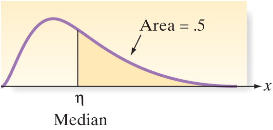
Figure 6.26
Location of the population median,
For example, increasing numbers of both private and public agencies are requiring their employees to submit to tests for substance abuse. One laboratory that conducts such testing has developed a system with a normalized measurement scale in which values less than 1.00 indicate “normal” ranges and values equal to or greater than 1.00 are indicative of potential substance abuse. The lab reports a normal result as long as the median level for an individual is less than 1.00. Eight independent measurements of each individual’s sample are made. One individual’s results are shown in Table 6.7.
Table 6.7 Substance Abuse Test Results

Alternate View
| .78 | .51 | 3.79 | .23 | .77 | .98 | .96 | .89 |
 Data Set: ABUSE
If the objective is to determine whether the population median (i.e., the true median level if an infinitely large number of measurements were made on the same individual sample) is less than 1.00, we establish that as our alternative hypothesis and test
The one-tailed sign test is conducted by counting the number of sample measurements that “favor” the alternative hypothesis—in this case, the number that are less than 1.00. If the null hypothesis is true, we expect approximately half of the measurements to fall on each side of the hypothesized median, and if the alternative is true, we expect significantly more than half to favor the alternative—that is, to be less than 1.00. Thus,
If we wish to conduct the test at the level of significance, the rejection region can be expressed in terms of the observed significance level, or p-value, of the test:
In this example, of the 8 measurements are less than 1.00. To determine the observed significance level associated with that outcome, we note that the number of measurements less than 1.00 is a binomial random variable (check the binomial characteristics presented in Chapter 4), and if is true, the binomial probability p that a measurement lies below (or above) the median 1.00 is equal to .5 (Figure 6.26). What is the probability that a result is as contrary to or more contrary to than the one observed? That is, what is the probability that 7 or more of 8 binomial measurements will result in Success (be less than 1.00) if the probability of Success is .5? Binomial Table I in Appendix B (with and ) indicates that
Thus, the probability that at least 7 of 8 measurements would be less than 1.00 if the true median were 1.00 is only .035. The p-value of the test is therefore .035.
This p-value can also be obtained from a statistical software package. The MINITAB printout of the analysis is shown in Figure 6.27, with the p-value highlighted. Since is less than we conclude that this sample provides sufficient evidence to reject the null hypothesis. The implication of this rejection is that the laboratory can conclude at the level of significance that the true median level for the individual tested is less than 1.00. However, we note that one of the measurements, with a value of 3.79, greatly exceeds the others and deserves special attention. This large measurement is an outlier that would make the use of a t-test and its concomitant assumption of normality dubious. The only assumption necessary to ensure the validity of the sign test is that the probability distribution of measurements is continuous.

Figure 6.27
MINITAB printout of sign test
The use of the sign test for testing hypotheses about population medians is summarized in the following box.
Nonparametric Sign Test for a Population Median, η
Let
[Note: Eliminate measurements that are exactly equal to .]
| One-Tailed Tests | Two-Tailed Test | ||
|---|---|---|---|
| Test statistic: | |||
| p-value: | |||
Decision: Reject H0 if
where and x has a binomial distribution with parameters n and . (See Table I, Appendix B.)
Conditions Required for a Valid Application of the Sign Test
The sample is selected randomly from a continuous probability distribution.
[Note: No assumptions need to be made about the shape of the probability distribution.]
Recall that the normal probability distribution provides a good approximation of the binomial distribution when the sample size is large (i.e., when both and ). For tests about the median of a distribution, the null hypothesis implies that and the normal distribution provides a good approximation if (Note that for and ) Thus, we can use the standard normal z-distribution to conduct the sign test for large samples. The large-sample sign test is summarized in the next box.
Large-Sample Sign Test for a Population Median,
Let population median
of sample measurements below ,
of sample measurements above
[Note: Eliminate measurements that are exactly equal to .]
| One-Tailed Tests | Two-Tailed Test | ||
|---|---|---|---|
| Test statistic: | |||
| where | |||
| Rejection region: | |||
| p-value: | |||
Decision: Reject H0 if or test statistic falls into the rejection region where and tabulated z values are found in Table II, Appendix B.
Example 6.14 Sign Test Application—Charge Length of iPod Batteries
Problem
A manufacturer of iPod batteries has established that the median time it takes for a battery to lose its charge is 10 hours. A sample of 40 iPod batteries from a competitor is obtained, and the batteries are tested continuously until each fails to hold a charge. Of the 40 failure times, 24 exceed 10 hours. Is there evidence that the median failure time of the competitor’s product differs from 10 hours? Use
Solution
The null and alternative hypotheses of interest are
Since we use the standard normal z-statistic:
Here, S is the maximum of (the number of measurements greater than 10) and (the number of measurements less than 10). Also,
Assumptions: The probability distribution of the failure times is continuous (time is a continuous variable), but nothing is assumed about its shape.
Since the number of measurements exceeding 10 is it follows that the number of measurements less than 10 is Consequently, the greater of and The calculated z-statistic is therefore
The value of z is not in the rejection region, so we cannot reject the null hypothesis at the level of significance.
Look Back
The manufacturer should not conclude, on the basis of this sample, that its competitor’s iPod batteries have a median failure time that differs from 10 hours. The manufacturer will not “accept ” however, since the probability of a Type II error is unknown.
Now Work Exercise 6.119
The one-sample nonparametric sign test for a median provides an alternative to the t-test for small samples from nonnormal distributions. However, if the distribution is approximately normal, the t-test provides a more powerful test about the central tendency of the distribution.
Exercises 6.115–6.131
Understanding the Principles
6.115 Under what circumstances is the sign test preferred to the t-test for making inferences about the central tendency of a population?
6.116 What is the probability that a randomly selected observation exceeds the
Mean of a normal distribution?
Median of a normal distribution?
Mean of a nonnormal distribution?
Median of a nonnormal distribution?
Learning the Mechanics
6.117 Use Table I of Appendix B or statistical software to calculate the following binomial probabilities:
when and
when and
when and
when and Also, use the normal approximation to calculate this probability, and then compare the approximation with the exact value.
when and Also, use the normal approximation to calculate this probability, and then compare the approximation with the exact value.
 L06118 6.118 Consider the following sample of 10 measurements:
Alternate View
8.4 16.9 15.8 12.5 10.3 4.9 12.9 9.8 23.7 7.3 Use these data, the binomial tables (Table I Appendix B) or statistical software, and to conduct each of the following sign tests:
Repeat each of the preceding tests, using the normal approximation to the binomial probabilities. Compare the results.
What assumptions are necessary to ensure the validity of each of the preceding tests?
 6.119 Suppose you wish to conduct a test of the research hypothesis that the median of a population is greater than 80. You randomly sample 25 measurements from the population and determine that 16 of them exceed 80. Set up and conduct the appropriate test of hypothesis at the .10 level of significance. Be sure to specify all necessary assumptions.
Applying the Concepts—Basic
- PAI 6.120 Music performance anxiety. Refer to the British Journal of Music Education (Mar. 2014) study of performance anxiety by music students, Exercise 6.60 (p. 335). Recall that the Performance Anxiety Inventory (PAI) was used to measure music performance anxiety on a scale from 20 to 80 points. The table below gives PAI values for participants in eight different studies. In Exercise 6.60 , you used the small-sample t-statistic to test whether the mean PAI value for all similar studies of music performance anxiety exceeds 40. However, the population of PAI values is unlikely to be normally distributed; consequently, inferences derived from the t-test may not be valid. Now consider a nonparametric test of the data.

Alternate View
54 42 51 39 41 43 55 40 Source: Patston, T. “Teaching stage fright?—Implications for music educators,” British Journal of Music Education, Vol. 31, No. 1, Mar. 2014 (adapted from Figure 1).
Set up the null and alternative hypotheses for determining whether the population median PAI value, , exceeds 40.
Find the rejection region for the test, part a, using .
Compute the test statistic.
State the appropriate conclusion for the test.
Find the p-value for the nonparametric test and use it to make a conclusion. (Your conclusion should agree with your answer in part d.)
How would your conclusion change if you used ?
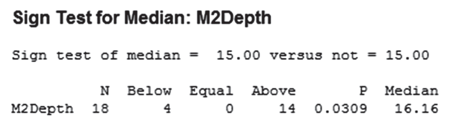
- MOLARS 6.121 Cheek teeth of extinct primates. Refer to the American Journal of Physical Anthropology (Vol. 142, 2010) study of the characteristics of cheek teeth (e.g., molars) in an extinct primate species, Exercise 2.38 (p. 50). Recall that the researchers measured the dentary depth of molars (in millimeters) for 18 cheek teeth extracted from skulls. These depth measurements are reproduced in accompanying table. The researchers are interested in the median molar depth of all cheek teeth from this extinct primate species. In particular, they want to know if the population median differs from 15 mm.
Specify the null and alternative hypotheses of interest of the researchers.
Explain why the sign test is appropriate to apply in this case.
A MINITAB printout of the analysis is shown below. Locate the test statistic on the printout.

Alternate View
18.12 19.48 19.36 15.94 15.83 19.70 15.76 17.00 16.20 13.96 16.55 15.70 17.83 13.25 16.12 18.13 14.02 14.04 Based on Boyer, D. M., Evans, A. R., and Jernvall, J. “Evidence of dietary differentiation among Late Paleocene–Early Eocene Plesiadapids (Mammalia, Primates).” American Journal of Physical Anthropology, Vol. 142, ©2010 (Table A3).
Find the p-value on the printout, and use it to draw a conclusion. Test using .
- STARBKS 6.122 Caffeine in Starbucks coffee. Scientists at the University of Florida College of Medicine investigated the level of caffeine in 16-ounce cups of Starbucks coffee (Journal of Analytical Toxicology, Oct. 2003). In one phase of the experiment, cups of Starbucks Breakfast Blend (a mix of Latin American coffees) were purchased on six consecutive days from a single specialty coffee shop. The amount of caffeine in each of the six cups (measured in milligrams) is provided in the following table.

Alternate View
564 498 259 303 300 307 Suppose the scientists are interested in determining whether the median amount of caffeine in Breakfast Blend coffee exceeds 300 milligrams. Set up the null and alternative hypotheses of interest.
How many of the cups in the sample have a caffeine content that exceeds 300 milligrams?
Assuming that use the binomial table in Appendix B or statistical software to find the probability that at least 4 of the 6 cups have caffeine amounts that exceed 300 milligrams.
On the basis of the probability you found in part c, what do you conclude about and (Use )
6.123 Emotional empathy in young adults. Refer to the Journal of Moral Education (June 2010) study of emotional empathy in young adults, Exercise 6.39 (p. 329). Recall that psychologists theorize that young female adults show more emotional empathy towards others than do males. To test the theory, each in a sample of 30 female college students responded to the following statement on emotional empathy: “I often have tender, concerned feelings for people less fortunate than me.” Responses (i.e., empathy scores) ranged from 0 to 4, where “never” and “always.” Suppose it is known that male college students have a median emotional empathy score of
Specify the null and alternative hypotheses for testing whether female college students have a median emotional empathy scale score higher than 2.8.
Suppose that distribution of emotional empathy scores for the 30 female students is as shown in the table below. Use this information to compute the test statistic.
Find the observed significance level (p-value) of the test.
At , what is the appropriate conclusion?
Response (empathy score) Number of Females 0 1 1 3 2 5 3 12 4 9
6.124 Quality of white shrimp. In The American Statistician (May 2001), the nonparametric sign test was used to analyze data on the quality of white shrimp. One measure of shrimp quality is cohesiveness. Since freshly caught shrimp are usually stored on ice, there is concern that cohesiveness will deteriorate after storage. For a sample of 20 newly caught white shrimp, cohesiveness was measured both before and after storage on ice for two weeks. The difference in the cohesiveness measurements (before minus after) was obtained for each shrimp. If storage has no effect on cohesiveness, the population median of the differences will be 0. If cohesiveness deteriorates after storage, the population median of the differences will be positive.
Set up the null and alternative hypotheses to test whether cohesiveness will deteriorate after storage.
In the sample of 20 shrimp, there were 13 positive differences. Use this value to find the p-value of the test.
Make the appropriate conclusion (in the words of the problem) if
- MTBE 6.125 Groundwater contamination of wells. Methyl tert-butyl ether (MTBE) is a lead fuel additive that can contaminate drinking water through leaking underground storage tanks at gasoline stations. A study published in Environmental Science & Technology (Jan. 2005) investigated the risk of exposure to MTBE through drinking water in New Hampshire. Data were collected for a sample of 223 public and private New Hampshire wells. Suppose environmental regulations stipulate that only half the wells in the state should have MTBE levels that exceed .5 micrograms per liter. This implies that the median MTBE level should be less than .5. Do the data collected by the researchers (saved in the MTBE file) provide evidence to indicate that the median level of MTBE in New Hampshire groundwater wells is less than .5 micrograms per liter? Use the accompanying MINITAB printout to answer the question.

Applying the Concepts—Intermediate
- SPIDER 6.126 Crab spiders hiding on flowers. Refer to the Behavioral Ecology (Jan. 2005) field study on the natural camouflage of crab spiders, presented in Exercise 2.42 (p. 51). Ecologists collected a sample of 10 adult female crab spiders, each sitting on the yellow central part of a daisy, and measured the chromatic contrast between each spider and the flower. The contrast values for the 10 crab spiders are reproduced in the table. (Note: The lower the contrast, the more difficult it is for predators to see the crab spider on the flower.) Recall that a contrast of 70 or greater allows bird predators to see the spider. Consider a test to determine whether the population median chromatic contrast of spiders on flowers is less than 70.

Alternate View
57 75 116 37 96 61 56 2 43 32 Based on Thery, M., et al. “Specific color sensitivities of prey and predator explain camouflage in different visual systems.” Behavioral Ecology, Vol. 16, No. 1, Jan. 2005 (Table 1).
State the null and alternative hypotheses for the test of interest.
Calculate the value of the test statistic.
Find the p-value for the test.
At what is the appropriate conclusion? State your answer in the words of the problem.
- TRAPS 6.127 Lobster trap placement. Refer to the Bulletin of Marine Science (Apr. 2010) observational study of lobster trap placement by teams fishing for the red spiny lobster in Baja California Sur, Mexico, Exercise 6.59 (p. 335). Trap spacing measurements (in meters) for a sample of seven teams of red spiny lobster fishermen are reproduced in the accompanying table. In Exercise 6.59 , you tested whether the average of the trap spacing measurements for the population of red spiny lobster fishermen fishing in Baja California Sur, Mexico, differs from 95 meters.

Alternate View
93 99 105 94 82 70 86 Based on Shester, G. G. “Explaining catch variation among Baja California lobster fishers through spatial analysis of trap-placement decisions.” Bulletin of Marine Science, Vol. 86, No. 2, Apr. 2010 (Table 1).
There is concern that the trap spacing data do not follow a normal distribution. If so, how will this impact the test you conducted in Exercise 6.59 ?
Propose an alternative nonparametric test to analyze the data.
Compute the value of the test statistic for the nonparametric test.
Find the p-value of the test.
Use the value of you selected in Exercise 6.59 and give the appropriate conclusion.
- ROCKS 6.128 Characteristics of a rockfall. Refer to the Environmental Geology (Vol. 58, 2009) simulation study of how far a block from a collapsing rockwall will bounce down a soil slope, Exercise 2.61 (p. 61). Recall that the variable of interest was rebound length (measured in meters) of the falling block. Based on the depth, location, and angle of block-soil impact marks left on the slope from an actual rockfall, the 13 rebound lengths shown in the table in the next column were estimated. Consider the following statement: “In all similar rockfalls, half of the rebound lengths will exceed 10 meters.” Is this statement supported by the sample data? Test using
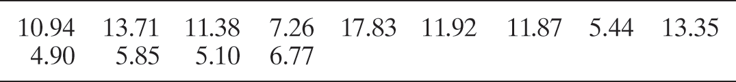
Alternate View
10.94 13.71 11.38 7.26 17.83 11.92 11.87 5.44 13.35 4.90 5.85 5.10 6.77 Based on Paronuzzi, P. “Rockfall-induced block propagation on a soil slope, northern Italy.” Environmental Geology, Vol. 58, 2009 (Table 2).
- RECALL 6.129 Free recall memory strategy. Refer to the Advances in Cognitive Psychology (Oct. 2012) study of free recall memory, Exercise 6.67 (p. 337). Recall that each in a sample of 8 participants memorized a list of items using the category clustering strategy and the ratio of repetition was recorded for each participant. These ratios are reproduced in the table. Is there evidence to indicate that the median ratio of repetition for all participants in a similar memory study differs from .5? Select an appropriate Type I error rate for your test and compare your results to those from Exercise 6.67 .

Alternate View
.25 .43 .57 .38 .38 .60 .47 .30 Source: Senkova, O., and Otani, H. “Category clustering calculator for free recall.” Advances in Cognitive Psychology, Vol. 8, No. 4, Oct. 2012 (Table 3).
- TOMBS 6.130 Radon exposure in Egyptian tombs. Refer to the Radiation Protection Dosimetry (Dec. 2010) study of radon exposure in Egyptian tombs, Exercise 6.64 (p. 336). The radon levels—measured in becquerels per cubic meter (Bq/m3)—in the inner chambers of a sample of 12 tombs are reproduced in the table. Recall that for safety purposes, the Egypt Tourism Authority (ETA) temporarily closes the tombs if the level of radon exposure in the tombs is too high, say, 6,000 Bq/m3. Conduct a nonparametric test to determine if the true median level of radon exposure in the tombs is less than 6,000 Bq/m3. Use Should the tombs be closed?
Radon levels in Egyptian tombs

Alternate View
50 910 180 580 7800 4000 390 12100 3400 1300 11900 1100 - SKID 6.131 Minimizing tractor skidding distance. Refer to the Journal of Forest Engineering (July 1999) study of minimizing tractor skidding distances along a new road in a European forest, presented in Exercise 6.69 (p. 337). The skidding distances (in meters) were measured at 20 randomly selected road sites. The data are repeated in the accompanying table. In Exercise 6.69 , you conducted a test of hypothesis for the population mean skidding distance. Now conduct a test to determine whether the population median skidding distance is more than 400 meters. Use
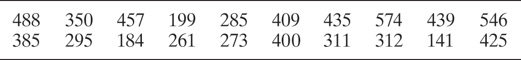
Alternate View
488 350 457 199 285 409 435 574 439 546 385 295 184 261 273 400 311 312 141 425 Based on Tujek, J., and Pacola, E. “Algorithms for skidding distance modeling on a raster Digital Terrain Model,” Journal of Forest Engineering, Vol. 10, No. 1, July 1999 (Table 1).