
Overall Transmission Structure
Abstract
The overall transmission structure in the time domain (frame, subframe, slots, OFDM symbols) and in the frequency domain (subcarrier, DC handling, bandwidth parts) is described in this chapter. Antenna ports, quasi-colocation, and duplex schemes are also discussed.
Keywords
Slot; subframe; frame; resource block; bandwidth part (BWP); quasi-colocation (QCL); antenna ports; frequency raster; carrier aggregation; supplementary uplink; FDD; TDD; slot format indication (SFI)
Prior to discussing the detailed NR downlink and uplink transmission schemes, a description of the basic time–frequency transmission resource of NR will be provided in this chapter, including bandwidth parts, supplementary uplink, carrier aggregation, duplex schemes, antenna ports, and quasi-colocation.
7.1 Transmission Scheme
OFDM was found to be a suitable waveform for NR due to its robustness to time dispersion and ease of exploiting both the time and frequency domains when defining the structure for different channels and signals. It is therefore the basic transmission scheme for both the downlink and uplink transmission directions in NR. However, unlike LTE where DFT-precoded OFDM is the sole transmission scheme in the uplink, NR uses OFDM as the baseline uplink transmission scheme with the possibility for complementary DFT-precoded OFDM. The reasons for DFT-precoded OFDM in the uplink are the same as in LTE, namely to reduce the cubic metric and obtain a higher power-amplifier efficiency, but the use of DFT-precoding also has several drawbacks including:
- • Spatial multiplexing (“MIMO”) receivers become more complex. This was not an issue when DFT-precoding was agreed in the first LTE release as it did not support uplink spatial multiplexing but becomes important when supporting uplink spatial multiplexing.
- • Maintaining symmetry between uplink and downlink transmission schemes is in many cases beneficial, something which is lost with an DFT-precoded uplink. One example of the benefits with symmetric schemes is sidelink transmission, that is, direct transmissions between devices. When sidelinks were introduced in LTE, it was agreed to keep the uplink transmission scheme which requires the devices to implement a receiver for DFT-precoded OFDM in addition to the OFDM receiver being already equipped for downlink transmissions. Introducing sidelink support in NR in the future is thus simpler as the device already has support for OFDM transmission and reception.
- • DFT-precoded OFDM implies scheduling restrictions as only contiguous allocations in the frequency domain are possible. In many cases this is an acceptable restriction, but there are also situations when it is desirable to use a noncontiguous allocation, for example, to obtain frequency diversity.
Hence, NR has adopted OFDM in the uplink with complementary support for DFT-precoding for data transmission. When DFT-precoding is used, uplink transmissions are restricted to a single layer only, while uplink transmissions of up to four layers are possible with OFDM. Support for DFT-precoding is mandatory in the device and the network can therefore configure DFT-precoding if/when needed. The waveform to use for the uplink random-access messages is configured as part of the system information.
One important aspect of OFDM is the selection of the numerology, in particular the subcarrier spacing and the cyclic prefix length. A large subcarrier spacing is beneficial from a frequency-error perspective as it reduces the impact from frequency errors and phase noise. However, for a certain cyclic prefix length in microseconds, the relative overhead increases the larger the subcarrier spacing and from this perspective a smaller cyclic prefix would be preferable. The selection of the subcarrier spacing therefore needs to carefully balance overhead from the cyclic prefix against sensitivity to Doppler spread/shift and phase noise.
For LTE, a choice of 15 kHz subcarrier spacing and a cyclic prefix of approximately 4.7 µs was found to offer a good balance between these different constraints for scenarios for which LTE was originally designed—outdoor cellular deployments up to approximately 3 GHz carrier frequency.
NR, on the other hand, is designed to support a wide range of deployment scenarios, from large cells with sub-1 GHz carrier frequency up to mm-wave deployments with very wide spectrum allocations. Having a single numerology for all these scenarios is not efficient or even possible. For the lower range of carrier frequencies, from below 1 GHz up to a few GHz, the cell sizes can be relatively large and a cyclic prefix capable of handling the delay spread expected in these type of deployments, a couple of microseconds, is necessary. Consequently, a subcarrier spacing in the LTE range or somewhat higher, in the range of 15–30 kHz, is needed. For higher carrier frequencies approaching the mm-wave range, implementation limitations such as phase noise become more critical, calling for higher subcarrier spacings. At the same time, the expected cell sizes are smaller at higher frequencies as a consequence of the more challenging propagation conditions. The extensive use of beamforming at high frequencies also helps reduce the expected delay spread. Hence, for these types of deployments a higher subcarrier spacing and a shorter cyclic prefix are suitable.
From the discussion above it is seen that a scalable numerology is needed. NR therefore supports a flexible numerology with a range of subcarrier spacings, based on scaling a baseline subcarrier spacing of 15 kHz. The reason for the choice of 15 kHz is coexistence with LTE and the LTE-based NB-IoT on the same carrier. This is an important requirement, for example, for an operator which has deployed NB-IoT or eMTC to support machine-type communication. Unlike smartphones, such MTC devices can have a relatively long replacement cycle, 10 years or longer. Without provisioning for coexistence, the operator would not be able to migrate the carrier to NR until all the MTC devices have been replaced. Another example is gradual migration where the limited spectrum availability may force an operator to share a single carrier between LTE and NR in the time domain. LTE coexistence is further discussed in Chapter 17.
Consequently, 15 kHz subcarrier spacing was selected as the baseline for NR. From the baseline subcarrier spacing, subcarrier spacings ranging from 15 kHz up to 240 kHz with a proportional change in cyclic prefix duration as shown in Table 7.1 are derived. Note that 240 kHz is supported for the SS block only (see Section 16.1), and not for regular data transmission. Although the NR physical-layer specification is band-agnostic, not all supported numerologies are relevant for all frequency bands. For each frequency band, radio requirements are therefore defined for a subset of the supported numerologies as discussed in Chapter 18, RF Characteristics and Requirements.
Table 7.1
| Subcarrier Spacing (kHz) | Useful Symbol Time, Tu (µs) | Cyclic Prefix, TCP (µs) |
|---|---|---|
| 15 | 66.7 | 4.7 |
| 30 | 33.3 | 2.3 |
| 60 | 16.7 | 1.2 |
| 120 | 8.33 | 0.59 |
| 240 | 4.17 | 0.29 |
To provide consistent and exact timing definitions, different time intervals within the NR specifications are defined as multiples of a basic time unit Tc=1/(480000·4096). The basic time unit Tc can thus be seen as the sampling time of an FFT-based transmitter/receiver implementation for a subcarrier spacing of 480 kHz with an FFT size equal to 4096. This is similar to the approach taken in LTE, which uses a basic time unit Ts=64Tc.
As discussed above, the choice of 15 kHz subcarrier spacing is motivated by coexistence with LTE. Efficient coexistence also requires alignment in the time domain and for this reason the NR slot structure for 15 kHz is identical to the LTE subframe structure. This means that the cyclic prefix for the first and eighth symbols are somewhat larger than for the other symbols. The slot structure for higher subcarrier spacings in NR is then derived by scaling this baseline structure by powers of two. In essence, an OFDM symbol is split into two OFDM symbols of the next higher numerology (see Fig. 7.1). Scaling by powers of two is beneficial as it maintains the symbol boundaries across numerologies, which simplifies mixing different numerologies on the same carrier. For the OFDM symbols with a somewhat larger cyclic prefix, the excess samples are allocated to the first of the two symbols obtained when splitting one symbol.

The useful symbol time Tu depends on the subcarrier spacing as shown in Table 7.1, with the overall OFDM symbol time being the sum of the useful symbol time and the cyclic-prefix length TCP. In LTE, two different cyclic prefixes are defined, normal cyclic prefix and extended cyclic prefix. The extended cyclic prefix, although less efficient from a cyclic-prefix-overhead point of view, was intended for specific environments with excessive delay spread where performance was limited by time dispersion. However, extended cyclic prefix was not used in practical deployments (except for MBSFN transmission), rendering it an unnecessary feature in LTE for unicast transmission. With this in mind, NR defines a normal cyclic prefix only, with the exception of 60 kHz subcarrier spacing, where both normal and extended cyclic prefix are defined for reasons discussed below.
7.2 Time-Domain Structure
In the time domain, NR transmissions are organized into frames of length 10 ms, each of which is divided into 10 equally sized subframes of length 1 ms. A subframe is in turn divided into slots consisting of 14 OFDM symbols each, that is, the duration of a slot in milliseconds depends on the numerology as illustrated in Fig. 7.2. On a higher level, each frame is identified by a system frame number (SFN). The SFN is used to define different transmission cycles that have a period longer than one frame, for example, paging sleep-mode cycles. The SFN period equals 1024, thus the SFN repeats itself after 1024 frames or 10.24 s.

For the 15 kHz subcarrier spacing, an NR slot thus has the same structure as an LTE subframe with normal cyclic prefix, which is beneficial from a coexistence perspective as discussed above. Note that a subframe in NR serves as a numerology-independent time reference, which is useful, especially in the case of multiple numerologies being mixed on the same carrier, while a slot is the typical dynamic scheduling unit. In contrast, LTE with its single subcarrier spacing uses the term subframe for both these purposes.
Since a slot is defined as a fixed number of OFDM symbols, a higher subcarrier spacing leads to a shorter slot duration. In principle this can be used to support lower-latency transmission, but as the cyclic prefix also shrinks when increasing the subcarrier spacing, it is not a feasible approach in all deployments. Therefore, to facilitate a fourfold reduction in the slot duration and the associated delay while maintaining a cyclic prefix similar to the 15 kHz case, an extended cyclic prefix is defined for 60 kHz subcarrier spacing. However, it comes at the cost of increased overhead in terms of cyclic prefix and is a less efficient way of providing low latency. The subcarrier spacing is therefore primarily selected to meet the deployment scenario in terms of, for example, carrier frequency, expected delay spread in the radio channel, and any coexistence requirements with LTE-based systems on the same carrier.
An alternative and more efficient way to support low latency is to decouple the transmission duration from the slot duration. Instead of changing subcarrier spacing and/or slot duration, the latency-critical transmission uses whatever number of OFDM symbols necessary to deliver the payload. NR therefore supports occupying only part of a slot for the transmission, sometimes referred to as “mini-slot transmission.” In other words, the term slot is primarily a numerology-dependent time reference and only loosely coupled with the actual transmission duration.
There are multiple reasons why it is beneficial to allow transmission to occupy only a part of a slot as illustrated in Fig. 7.3. One reason is, as already discussed, support of very low latency. Such transmissions can also preempt an already ongoing, longer transmission to another device as discussed in Section 14.1.2, allowing for immediate transmission of data requiring very low latency.

Another reason is support for analog beamforming as discussed in Chapters 11 and 12 where at most one beam at a time can be used for transmission. Different devices therefore need to be time-multiplexed and with the very large bandwidths available in the mm-wave range, a few OFDM symbols can be sufficient even for relatively large payloads.
A third reason is operation in unlicensed spectra. Unlicensed operation is not part of release 15 but will be introduced in a later release. In unlicensed spectra, listen-before-talk is typically used to ensure the radio channel is available for transmission. Once the listen-before-talk operation has declared the channel available, it is beneficial to start transmission immediately to avoid another device occupying the channel. If data transmission would have to wait until the start of a slot boundary, some form of dummy data or reservation signal needs to be transmitted from the successful listen-before-talk operation until the start of the slot, which would degrade the efficiency of the system.
7.3 Frequency-Domain Structure
When the first release of LTE was designed, it was decided that all devices should be capable of the maximum carrier bandwidth of 20 MHz, which was a reasonable assumption at the time given the relatively modest bandwidth, compared to NR. On the other hand, NR is designed to support very wide bandwidths, up to 400 MHz for a single carrier. Mandating all devices to handle such wide carriers is not reasonable from a cost perspective. Hence, an NR device may see only a part of the carrier and, for efficient utilization of the carrier, the part of the carrier received by the device may not be centered around the carrier frequency. This has implications for, among other things, the handling of the DC subcarrier.
In LTE, the DC subcarrier is not used as it may be subject to disproportionally high interference due to, for example, local-oscillator leakage. Since all LTE devices can receive the full carrier bandwidth and are centered around the carrier frequency, this was straightforward.1 NR devices, on the other hand, may not be centered around the carrier frequency and each NR device may have its DC located at different locations in the carrier, unlike LTE where all devices typically have the DC coinciding with the center of the carrier. Therefore, having special handling of the DC subcarrier would be cumbersome in NR and instead it was decided to exploit also the DC subcarrier for data as illustrated in Fig. 7.4, accepting that the quality of this subcarrier may be degraded in some situations.

A resource element, consisting of one subcarrier during one OFDM symbol, is the smallest physical resource in NR. Furthermore, as illustrated in Fig. 7.5, 12 consecutive subcarriers in the frequency domain are called a resource block.

Note that the NR definition of a resource block differs from the LTE definition. An NR resource block is a one-dimensional measure spanning the frequency domain only, while LTE uses two-dimensional resource blocks of 12 subcarriers in the frequency domain and one slot in the time domain. One reason for defining resource blocks in the frequency domain only in NR is the flexibility in time duration for different transmissions whereas, in LTE, at least in the original release, transmissions occupied a complete slot.2
NR supports multiple numerologies on the same carrier and, consequently, there are multiple resource sets of resource grids, one for each numerology (Fig. 7.6). Since a resource block is 12 subcarriers, the frequency span measured in Hz is different. The resource block boundaries are aligned across numerologies such that two resource blocks at a subcarrier spacing of Δf occupy the same frequency range as one resource block at a subcarrier spacing of 2Δf. In the NR specifications, the alignment across numerologies in terms of resource block boundaries, as well as symbol boundaries, is described through multiple resource grids where there is one resource grid per subcarrier spacing and antenna port (see Section 7.9 for a discussion of antenna ports), covering the full carrier bandwidth in the frequency domain and one subframe in the time domain.

The resource grid models the transmitted signal as seen by the device for a given subcarrier spacing. However, the device needs to know where in the carrier the resource blocks are located. In LTE, where there is a single numerology and all devices support the full carrier bandwidth, this is straightforward. NR, on the other hand, supports multiple numerologies and, as discussed further below in conjunction with bandwidth parts, not all devices may support the full carrier bandwidth. Therefore, a common reference point, known as point A, together with the notion of two types of resource blocks, common resource blocks and physical resource blocks, are used.3 Reference point A coincides with subcarrier 0 of common resource block 0 for all subcarrier spacings. This point serves as a reference from which the frequency structure can be described and point A may be located outside the actual carrier. Upon detecting an SS block as part of the initial access (see Section 16.1), the device is signalled the location of point A as part of the broadcast system information (SIB1).
The physical resource blocks, which are used to describe the actual transmitted signal, are then located relative to this reference point, as illustrated in Fig. 7.7. For example, physical resource block 0 for subcarrier spacing Δf is located m resource blocks from reference point A or, expressed differently, corresponds to common resource block m. Similarly, physical resource block 0 for subcarrier spacing 2Δf corresponds to common resource block n. The starting points for the physical resource blocks are signaled independently for each numerology (m and n in the example in Fig. 7.7), a feature that is useful for implementing the filters necessary to meet the out-of-band emission requirements (see Chapter 18). The guard in Hz needed between the edge of the carrier and the first used subcarrier is larger, the larger the subcarrier spacing, which can be accounted for by independently setting the offset between the first used resource block and reference point A. In the example in Fig. 7.7, the first used resource block for subcarrier spacing 2Δf is located further from the carrier edge than for subcarrier spacing Δf to avoid excessively steep filtering requirements for the higher numerology or, expressed differently, to allow a larger fraction of the spectrum to be used for the lower subcarrier spacing.

The location of the first usable resource block, which is the same as the start of the resource grid in the frequency domain, is signaled to the device. Note that this may or may not be the same as the first resource block of a bandwidth part (bandwidth parts are described in Section 7.4).
An NR carrier should at most be 275 resource blocks wide, which corresponds to 275·12=3300 used subcarriers. This also defines the largest possible carrier bandwidth in NR for each numerology. However, there is also an agreement to limit the per-carrier bandwidth to 400 MHz, resulting in the maximum carrier bandwidths of 50/100/200/400 MHz for subcarrier spacings of 15/30/60/120 kHz, respectively, as mentioned in Chapter 5. The smallest possible carrier bandwidth of 11 resource blocks is given by the RF requirements on spectrum utilization (see Chapter 18). However, for the numerology used for the SS block (see Chapter 16) at least 20 resource blocks are required in order for the device to be able to find and synchronize to the carrier.
7.4 Bandwidth Parts
As discussed above, LTE is designed under the assumption that all devices are capable of the maximum carrier bandwidth of 20 MHz. This avoided several complications, for example, around the handling of the DC subcarrier as already discussed, while having a negligible impact on the device cost. It also allowed control channels to span the full carrier bandwidth to maximize frequency diversity.
The same assumption—all devices being able to receive the full carrier bandwidth—is not reasonable for NR, given the very wide carrier bandwidth supported. Consequently, means for handling different device capabilities in terms of bandwidth support must be included in the design. Furthermore, reception of a very wide bandwidth can be costly in terms of device energy consumption compared to receiving a narrower bandwidth. Using the same approach as in LTE where the downlink control channels would occupy the full carrier bandwidth would therefore significantly increase the power consumption of the device. A better approach is, as done in NR, to use receiver-bandwidth adaptation such that the device can use a narrower bandwidth for monitoring control channels and to receive small-to-medium-sized data transmissions and to open the full bandwidth when a large amount of data is scheduled.
To handle these two aspects—support for devices not capable of receiving the full carrier bandwidth and receiver-side bandwidth adaptation—NR defines bandwidth parts (BWPs) (see Fig. 7.8). A bandwidth part is characterized by a numerology (subcarrier spacing and cyclic prefix) and a set of consecutive resource blocks in the numerology of the BWP, starting at a certain common resource block.

When a device enters the connected state it has obtained information from the PBCH about the control resource set (CORESET; see Section 10.1.2) where it can find the control channel used to schedule the remaining system information (see Chapter 16 for details). The CORESET configuration obtained from the PBCH also defines and activates the initial bandwidth part in the downlink. The initial active uplink bandwidth part is obtained from the system information scheduled using the downlink PDCCH.
Once connected, a device can be configured with up to four downlink bandwidth parts and up to four uplink bandwidth parts for each serving cell. In the case of SUL operation (see Section 7.7), there can be up to four additional uplink bandwidth parts on the supplementary uplink carrier.
On each serving cell, at a given time instant one of the configured downlink bandwidth parts is referred to as the active downlink bandwidth part for the serving cell and one of the configured uplink bandwidth parts is referred to as the active uplink bandwidth part for the serving cell. For unpaired spectra a device may assume that the active downlink bandwidth part and the active uplink bandwidth part of a serving cell have the same center frequency. This simplifies the implementation as a single oscillator can be used for both directions. The gNB can activate and deactivate bandwidth parts using the same downlink control signaling as for scheduling information (see Chapter 10), thereby achieving rapid switching between different bandwidth parts.
In the downlink, a device is not assumed to be able to receive downlink data transmissions, more specifically the PDCCH or PDSCH, outside the active bandwidth part. Furthermore, the numerology of the PDCCH and PDSCH are restricted to the numerology configured for the bandwidth part. Thus, in release 15, a device can only receive one numerology at a time as multiple bandwidth parts cannot be simultaneously active. Mobility measurements can still be done outside an active bandwidth part but require a measurement gap similarly to intercell measurements. Hence, a device is not expected to monitor downlink control channels while doing measurements outside the active bandwidth part.
In the uplink, a device transmits PUSCH and PUCCH in the active uplink bandwidth part only.
Given the above discussion, a relevant question is why two mechanisms, carrier aggregation and bandwidth parts, are defined instead of using the carrier-aggregation framework only. To some extent carrier aggregation could have been used to handle devices with different bandwidth capabilities as well as bandwidth adaptation. However, from an RF perspective there is a significant difference. A component carrier is associated with various RF requirements such as out-of-band emission requirements as discussed in Chapter 18, but for a bandwidth part inside a carrier there is no such requirement—it is all handled by the requirements set on the carrier as such. Furthermore, from an MAC perspective there are also some differences in the handling of, for example, hybrid ARQ retransmissions which cannot move between component carriers.
7.5 Frequency-Domain Location of NR Carriers
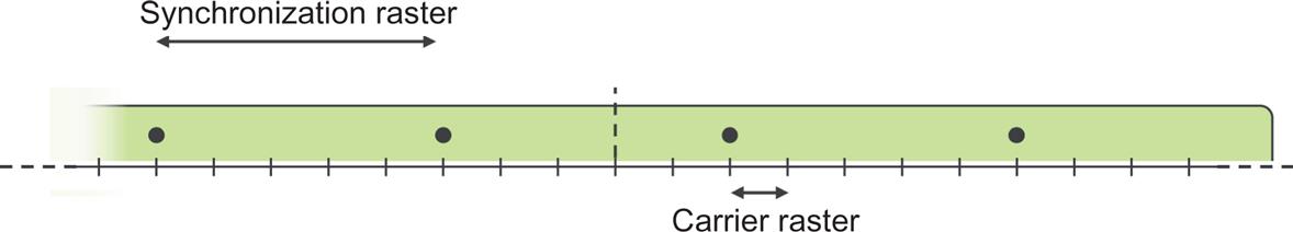
In principle, an NR carrier could be positioned anywhere within the spectrum and, similarly to LTE, the basic NR physical-layer specification does not say anything about the exact frequency location of an NR carrier, including the frequency band. However, in practice, there is a need for restrictions on where an NR carrier can be positioned in the frequency domain to simplify RF implementation and to provide some structure to carrier assignments in a frequency band between different operators. In LTE, a 100 kHz carrier raster served this purpose and a similar approach has been taken in NR. However, the NR raster has a much finer granularity of 5 kHz up to 3 GHz carrier frequency, 15 kHz for 3–24.25 GHz, and 60 kHz above 24.25 GHz. This raster has the benefit of being a factor in the subcarrier spacings relevant for each frequency range, as well as being compatible with the 100 kHz LTE raster in bands where LTE is deployed (below 3 GHz).
In LTE, this carrier raster also determines the frequency locations a device must search for as part of the initial access procedure. However, given the much wider carriers possible in NR and the larger number of bands in which NR can be deployed, as well as the finer raster granularity, performing initial cell search on all possible raster positions would be too time consuming. Instead, to reduce the overall complexity and not spend an unreasonable time on cell search, NR also defines a sparser synchronization raster, which is what an NR device has to search upon initial access. A consequence of having a sparser synchronization raster than carrier raster is that, unlike LTE, the synchronization signals may not be centered in the carrier (see Fig. 7.9 and Chapter 16 for further details).
7.6 Carrier Aggregation
The possibility of carrier aggregation is part of NR from the first release. Similar to LTE, multiple NR carriers can be aggregated and transmitted in parallel to/from the same device, thereby allowing for an overall wider bandwidth and correspondingly higher per-link data rates. The carriers do not have to be contiguous in the frequency domain but can be dispersed, both in the same frequency band as well as in different bands, resulting in three difference scenarios:
Although the overall structure is the same for all three cases, the RF complexity can be vastly different.
Up to 16 carriers, possibly of different bandwidths and different duplex schemes, can be aggregated allowing for overall transmission bandwidths of up 16·400 MHz=6.4 GHz, which is far beyond typical spectrum allocations.
A device capable of carrier aggregation may receive or transmit simultaneously on multiple component carriers while a device not capable of carrier aggregation can access one of the component carriers. Thus, in most respects and unless otherwise mentioned, the physical-layer description in the following chapters applies to each component carrier separately in the case of carrier aggregation. It is worth noting that in the case of interband carrier aggregation of multiple half-duplex (TDD) carriers, the transmission direction on different carriers does not necessarily have to be the same. This implies that a carrier-aggregation-capable TDD device may need a duplex filter, unlike the typical scenario for a noncarrier-aggregation-capable device.
In the specifications, carrier aggregation is described using the term cell, that is, a carrier-aggregation-capable device is able to receive and transmit from/to multiple cells. One of these cells is referred to as the primary cell (PCell). This is the cell which the device initially finds and connects to, after which one or more secondary cells (SCells) can be configured once the device is in connected mode. The secondary cells can be rapidly activated or deceived to meet the variations in the traffic pattern. Different devices may have different cells as their primary cell—that is, the configuration of the primary cell is device-specific. Furthermore, the number of carriers (or cells) does not have to be the same in uplink and downlink. In fact, a typical case is to have more carriers aggregated in the downlink than in the uplink. There are several reasons for this. There is typically more traffic in the downlink that in the uplink. Furthermore, the RF complexity from multiple simultaneously active uplink carriers is typically larger than the corresponding complexity in the downlink.
Scheduling grants and scheduling assignments can be transmitted on either the same cell as the corresponding data, known as self-scheduling, or on a different cell than the corresponding data, known as cross-carrier scheduling, as illustrated in Fig. 7.10. In most cases, self-scheduling is sufficient.

7.6.1 Control Signaling
Carrier aggregation uses L1/L2 control signaling for the same reason as when operating with a single carrier. The use of downlink controls signaling for scheduling information was touched upon in the previous section. There is also a need for uplink control signaling, for example, hybrid-ARQ acknowledgments to inform the gNB about the success or failure of downlink data reception. As baseline, all the feedback is transmitted on the primary cell, motivated by the need to support asymmetric carrier aggregation with the number of downlink carriers supported by a device unrelated to the number of uplink carriers. For a large number of downlink component carriers, a single uplink carrier may carry a large number of acknowledgments. To avoid overloading a single carrier, it is possible to configure two PUCCH groups where feedback relating to the first group is transmitted in the uplink of the PCell and feedback relating to the other group of carriers is transmitted on the primary second cell (PSCell) (Fig. 7.11).

If carrier aggregation is used, the device may receive and transmit on multiple carriers, but reception on multiple carriers is typically only needed for the highest data rates. It is therefore beneficial to inactivate reception of carriers not used while keeping the configuration intact. Activation and inactivation of component carriers can be done through MAC signaling (more specifically, MAC control elements, discussed in Section 6.4.4.1) containing a bitmap where each bit indicates whether a configured SCell should be activated or deactivated.
7.7 Supplementary Uplink
In addition to carrier aggregation, NR also supports so-called “supplementary uplink” (SUL). As illustrated in Fig. 7.12, SUL implies that a conventional downlink/uplink (DL/UL) carrier pair has an associated or supplementary uplink carrier with the SUL carrier typically operating in lower-frequency bands. As an example, a downlink/uplink carrier pair operating in the 3.5 GHz band could be complemented with a supplementary uplink carrier in the 800 MHz band. Although Fig. 7.12 seems to indicate that the conventional DL/UL carrier pair operates on paired spectra with frequency separation between the downlink and uplink carriers, it should be understood that the conventional carrier pair could equally well operate in unpaired spectra with downlink/uplink separation by means of TDD. This would, for example, be the case in an SUL scenario where the conventional carrier pair operates in the unpaired 3.5 GHz band.

While the main aim of carrier aggregation is to enable higher peak data rates by increasing the bandwidth available for transmission to/from a device, the typical aim of SUL is to extend uplink coverage, that is, to provide higher uplink data rates in power-limited situations, by utilizing the lower path loss at lower frequencies. Furthermore, in an SUL scenario the non-SUL uplink carrier is typically significantly more wideband compared to the SUL carrier. Thus, under good channel conditions such as the device located relatively close to the cell site, the non-SUL carrier typically allows for substantially higher data rates compared to the SUL carrier. At the same time, under bad channel conditions, for example, at the cell edge, a lower-frequency SUL carrier typically allows for significantly higher data rates compared to the non-SUL carrier, due to the assumed lower path loss at lower frequencies. Hence, only in a relatively limited area do the two carriers provide similar data rates. As a consequence, aggregating the throughput of the two carriers has in most cases limited benefits. At the same time, scheduling only a single uplink carrier at a time simplifies transmission protocols and in particular the RF implementation as various intermodulation issues is avoided.
Note that for carrier aggregation the situation is different:
- • The two (or more) carriers in a carrier-aggregation scenario are often of similar bandwidth and operating at similar carrier frequencies, making aggregation of the throughput of the two carriers more beneficial;
- • Each uplink carrier in a carrier aggregation scenario is operating with its own downlink carrier, simplifying the support for simultaneous scheduling of multiple uplink transmissions in parallel.
Hence, only one of SUL and non-SUL is transmitting and simultaneous SUL and non-SUL transmission from a device is not possible.
One SUL scenario is when the SUL carrier is located in the uplink part of paired spectrum already used by LTE (see Fig. 7.13). In other words, the SUL carrier exists in an LTE/NR uplink coexistence scenario (see also Chapter 17). In many LTE deployments, the uplink traffic is significantly less than the corresponding downlink traffic. As a consequence, in many deployments, the uplink part of paired spectra is not fully utilized. Deploying an NR supplementary uplink carrier on top of the LTE uplink carrier in such a spectrum is a way to enhance the NR user experience with limited impact on the LTE network.

Finally, a supplementary uplink can also be used to reduce latency. In the case of TDD, the separation of uplink and downlink in the time domain may impose restrictions on when uplink data can be transmitted. By combining the TDD carrier with a supplementary carrier in paired spectra, latency-critical data can be transmitted on the supplementary uplink immediately without being restricted by the uplink–downlink partitioning on the normal carrier.
7.7.1 Relation to Carrier Aggregation
Although SUL may appear similar to uplink carrier aggregation there are some fundamental differences.
In the case of carrier aggregation, each uplink carrier has its own associated downlink carrier. Formally, each such downlink carrier corresponds to a cell of its own and thus different uplink carriers in a carrier-aggregation scenario correspond to different cells (see left part of Fig. 7.14).

In contrast, in the case of SUL the supplementary uplink carrier does not have an associated downlink carrier of its own. Rather the supplementary carrier and the conventional uplink carrier share the same downlink carrier. As a consequence, the supplementary uplink carrier does not correspond to a cell of its own. Instead, in the SUL scenario there is a single cell with one downlink carrier and two uplink carriers (right part of Fig. 7.14).
It should be noted that in principle nothing prevents the combination of carrier aggregation, for example, a situation with carrier aggregation between two cells (two DL/UL carrier pairs) where one of the cells is an SUL cell with an additional supplementary uplink carrier. However, there are currently no band combinations defined for such carrier-aggregation/SUL combinations.
A relevant question is, if there is a supplementary uplink, is there such a thing as a supplementary downlink? The answer is yes—since the carrier aggregation framework allows for the number of downlink carriers to be larger than the number of uplink carriers, some of the downlink carriers can be seen as supplementary downlinks. One common scenario is to deploy an additional downlink carrier in unpaired spectra and aggregate it with a carrier in paired spectra to increase capacity and data rates. No additional mechanisms beyond carrier aggregation are needed and hence the term supplementary downlink is mainly used from a spectrum point of view as discussed in Chapter 3.
7.7.2 Control Signaling
In the case of supplementary-uplink operation, a device is explicitly configured (by means of RRC signaling) to transmit PUCCH on either the SUL carrier or on the conventional (non-SUL) carrier.
In terms of PUSCH transmission, the device can be configured to transmit PUSCH on the same carrier as PUCCH. Alternatively, a device configured for SUL operation can be configured for dynamic selection between the SUL carrier or the non-SUL carrier. In the latter case, the uplink scheduling grant will include an SUL/non-SUL indicator that indicates on what carrier the scheduled PUSCH transmission should be carried. Thus, in the case of supplementary uplink, a device will never transmit PUSCH simultaneously on both the SUL carrier and on the non-SUL carrier.
As described in Section 10.2, if a device is to transmit UCI on PUCCH during a time interval that overlaps with a scheduled PUSCH transmission on the same carrier, the device instead multiplexes the UCI onto PUSCH. The same rule is true for the SUL scenario, that is, there is not simultaneous PUSCH and PUCCH transmission even on different carriers. Rather, if a device is to transmit UCI on PUCCH one carrier (SUL or non-SUL) during a time interval that overlaps with a scheduled PUSCH transmission on either carrier (SUL or non SUL), the device instead multiplexes the UCI onto the PUSCH.
An alternative to supplementary uplink would be to rely on dual connectivity with LTE on the lower frequency and NR on the higher frequency. Uplink data transmission would in this case be handled by the LTE carrier with, from a data rate perspective, the benefits would be similar to supplementary uplink. However, in this case, the uplink control signaling related to NR downlink transmissions has to be handled by the high-frequency NR uplink carrier as each carrier pair has to be self-contained in terms of L1/L2 control signaling. Using a supplementary uplink avoids this drawback and allows L1/L2 control signaling to exploit the lower-frequency uplink. Another possibility would be to use carrier aggregation, but in this case a low-frequency downlink carrier has to be configured as well, something which may be problematic in the case of LTE coexistence.
7.8 Duplex Schemes
Spectrum flexibility is one of the key features of NR. In addition to the flexibility in transmission bandwidth, the basic NR structure also supports separation of uplink and downlink in time and/or frequency subject to either half duplex or full duplex operation, all using the same single frame structure. This provides a large degree of flexibility (Fig. 7.15):
- • TDD—uplink and downlink transmissions use the same carrier frequency and are separated in time only;
- • FDD—uplink and downlink transmissions use different frequencies but can occur simultaneously;
- • Half-duplex FDD—uplink and downlink transmissions are separated in frequency and time, suitable for simpler devices operating in paired spectra.

In principle, the same basic NR structure would also allow full duplex operation with uplink and downlink separated neither in time, nor in frequency, although this would result in a significant transmitter-to-receiver interference problem whose solution is still in the research stage and left for the future.
LTE also supported both TDD and FDD, but unlike the single frame structure used in NR, LTE used two different frame structure types used.4 Furthermore, unlike LTE where the uplink–downlink allocation does not change over time,5 the TDD operation for NR is designed with dynamic TDD as a key technology component.
7.8.1 Time-Division Duplex (TDD)
In the case of TDD operation, there is a single carrier frequency and uplink and downlink transmissions are separated in the time domain on a cell basis. Uplink and downlink transmissions are nonoverlapping in time, both from a cell and a device perspective. TDD can therefore be classified as half-duplex operation.
In LTE, the split between uplink and downlink resources in the time domain was semistatically determined and essentially remained constant over time. NR, on the other hand, uses dynamic TDD as the basis where (parts of) a slot can be dynamically allocated to either uplink or downlink as part of the scheduler decision. This enables following rapid traffic variations which are particularly pronounced in dense deployments with a relatively small number of users per base station. Dynamic TDD is particularly useful in small-cell and/or isolated cell deployments where the transmission power of the device and the base station is of the same order and the intersite interference is reasonable. If needed, the scheduling decisions between the different sites can be coordinated. It is much simpler to restrict the dynamics in the uplink–downlink allocation when needed and thereby have a more static operation than trying to add dynamics to a fundamentally static scheme, which was done when introducing eIMTA for LTE in release 12.
One example when intersite coordination is useful is a traditional macrodeployment. In such scenarios, a (more or less) static uplink–downlink allocation is a good choice as it avoids troublesome interference situations. Static or semistatic TDD operation is also necessary for handling coexistence with LTE, for example, when an LTE carrier and an NR carrier are using the same sites and the same frequency band. Such restrictions in the uplink–downlink allocation can easily be achieved as part of the scheduling implementation by using a fixed pattern in each base station. There is also a possibility to semistatically configure the transmission direction of some or all of the slots as discussed in Section 7.8.3, a feature that can allow for reduced device energy consumption as it is not necessary to monitor for downlink control channels in slots that are a priori known to be reserved for uplink usage.
An essential aspect of any TDD system, or half-duplex system in general, is the possibility to provide a sufficiently large guard period (or guard time), where neither downlink nor uplink transmissions occur. This guard period is necessary for switching from downlink to uplink transmission and vice versa and is obtained by using slot formats where the downlink ends sufficiently early prior to the start of the uplink. The required length of the guard period depends on several factors. First, it should be sufficiently large to provide the necessary time for the circuitry in base stations and the devices to switch from downlink to uplink. Switching is typically relatively fast, of the order of 20 µs or less, and in most deployments does not significantly contribute to the required guard time.
Second, the guard time should also ensure that uplink and downlink transmissions do not interfere at the base station. This is handled by advancing the uplink timing at the devices such that, at the base station, the last uplink subframe before the uplink-to-downlink switch ends before the start of the first downlink subframe. The uplink timing of each device can be controlled by the base station by using the timing advance mechanism, as will be elaborated upon in Chapter 15. Obviously, the guard period must be large enough to allow the device to receive the downlink transmission and switch from reception to transmission before it starts the (timing-advanced) uplink transmission (see Fig. 7.16). As the timing advance is proportional to the distance to the base station, a larger guard period is required when operating in large cells compared to small cells.

Finally, the selection of the guard period also needs to take interference between base stations into account. In a multicell network, intercell interference from downlink transmissions in neighboring cells must decay to a sufficiently low level before the base station can start to receive uplink transmissions. Hence, a larger guard period than is motivated by the cell size itself may be required as the last part of the downlink transmissions from distant base stations, otherwise it may interfere with uplink reception. The amount of guard period depends on the propagation environments, but in some macrocell deployments the interbase-station interference is a nonnegligible factor when determining the guard period. Depending on the guard period, some residual interference may remain at the beginning of the uplink period. Hence, it is beneficial to avoid placing interference-sensitive signals at the start of an uplink burst.
7.8.2 Frequency-Division Duplex (FDD)
In the case of FDD operation, uplink and downlink are carried on different carrier frequencies, denoted fUL and fDL in Fig. 7.15. During each frame, there is thus a full set of slots in both uplink and downlink, and uplink and downlink transmission can occur simultaneously within a cell. Isolation between downlink and uplink transmissions is achieved by transmission/reception filters, known as duplex filters, and a sufficiently large duplex separation in the frequency domain.
Even if uplink and downlink transmission can occur simultaneously within a cell in the case of FDD operation, a device may be capable of full-duplex operation or only half-duplex operation for a certain frequency band, depending on whether or not it is capable of simultaneous transmission/reception. In the case of full-duplex capability, transmission and reception may also occur simultaneously at a device, whereas a device capable of only half-duplex operation cannot transmit and receive simultaneously. Half-duplex operation allows for simplified device implementation due to relaxed or no duplex-filters. This can be used to reduce device cost, for example, for low-end devices in cost-sensitive applciations. Another example is operation in certain frequency bands with a very narrow duplex gap with correspondingly challenging design of the duplex filters. In this case, full duplex support can be frequency-band-dependent such that a device may support only half-duplex operation in certain frequency bands while being capable of full-duplex operation in the remaining supported bands. It should be noted that full/half-duplex capability is a property of the device; the base station can operate in full duplex irrespective of the device capabilities. For example, the base station can transmit to one device while simultaneously receiving from another device.
From a network perspective, half-duplex operation has an impact on the sustained data rates that can be provided to/from a single device as it cannot transmit in all uplink subframes. The cell capacity is hardly affected as typically it is possible to schedule different devices in uplink and downlink in a given subframe. No provisioning for guard periods is required from a network perspective as the network is still operating in full duplex and therefore is capable of simultaneous transmission and reception. The relevant transmission structures and timing relations are identical between full-duplex and half-duplex FDD and a single cell may therefore simultaneously support a mixture of full-duplex and half-duplex FDD devices. Since a half-duplex device is not capable of simultaneous transmission and reception, the scheduling decisions must take this into account and half-duplex operation can be seen as a scheduling restriction.
7.8.3 Slot Format and Slot-Format Indication
Returning to the slot structure discussed in Section 7.2, it is important to point out that there is one set of slots in the uplink and another set of slots in the downlink, the reason being the time offset between the two as a function of timing advance. If both uplink and downlink transmission would be described using the same slot, which is often seen in various illustrations in the literature, it would not be possible to specify the necessary timing difference between the two.
Depending on the whether the device is capable of full duplex, as is the case for FDD, or half duplex only, as is the case for TDD, a slot may not be fully used for uplink or downlink transmission. As an example, the downlink transmission in Fig. 7.16 had to stop prior to the end of the slot in order to allow for sufficient time to switch to downlink reception. Since the necessary time between downlink and uplink depends on several factors, NR defines a wide range of slot formats defining which parts of a slot are used for uplink or downlink. Each slot format represents a combination of OFDM symbols denoted downlink, flexible, and uplink, respectively. The reason for having a third state, flexible, will be discussed further below, but one usage is to handle the necessary guard period in half-duplex schemes. A subset of the slot formats supported by NR are illustrated in Fig. 7.17. As seen in the figure, there are downlink-only and uplink-only slot formats which are useful for full-duplex operation (FDD), as well as partially filled uplink and downlink slots to handle the case of half-duplex operation (TDD).

The name slot format is somewhat misleading as there are separate slots for uplink and downlink transmissions, each filled with data in such a way that there is no simultaneous transmission and reception in the case of TDD. Hence, the slot format for a downlink slot should be understood as downlink transmissions can only occur in “downlink” or “flexible” symbols, and in an uplink slot, uplink transmissions can only occur in “uplink” or “flexible” symbols. Any guard period necessary for TDD operation is taken from the flexible symbols.
One of the key features of NR is, as already mentioned, the support for dynamic TDD where the scheduler dynamically determines the transmission direction. Since a half-duplex device cannot transmit and receive simultaneously, there is a need to split the resources between the two directions. In NR, three different signaling mechanisms provide information to the device on whether the resources are used for uplink or downlink transmission:
Some or all of these mechanisms are used in combination to determine the instantaneous transmission direction as will be discussed below. Although the description below uses the term dynamic TDD, the framework can in principle be applied to half-duplex operation in general, including half-duplex FDD.
The first mechanism and the basic principle is for the device to monitor for control signaling in the downlink and transmit/receive according to the received scheduling grants/assignments. In essence, a half-duplex device would view each OFDM symbol as a downlink symbol unless it has been instructed to transmit in the uplink. It is up to the scheduler to ensure that a half-duplex device is not requested to simultaneously receive and transmit. For a full-duplex-capable device (FDD), there is obviously no such restriction and the scheduler can independently schedule uplink and downlink.
The general principle above is simple and provides a flexible framework. However, if the network knows a priori that it will follow a certain uplink–downlink allocation, for example, in order to provide coexistence with some other TDD technology or to fulfill some spectrum regulatory requirement, it can be advantageous to provide this information to the device. For example, if it is known to a device that a certain set of OFDM symbols is assigned to uplink transmissions, there is no need for the device to monitoring for downlink control signaling in the part of the downlink slots overlapping with these symbols. This can help reducing the device power consumption. NR therefore provides the possibility to optionally signal the uplink–downlink allocation through RRC signaling.
The RRC-signaled pattern classifies OFDM symbols as “downlink,” “flexible,” or “uplink.” For a half-duplex device, a symbol classified as “downlink” can only be used for downlink transmission with no uplink transmission in the same period of time. Similarly, a symbol classified as “uplink” means that the device should not expect any overlapping downlink transmission. “Flexible” means that the device cannot make any assumptions on the transmission direction. Downlink control signaling should be monitored and if a scheduling message is found, the device should transmit/receive accordingly. Thus, the fully dynamic scheme outlined above is equivalent to semistatically declaring all symbols as “flexible.”
The RRC-signaled pattern is expressed as a concatenation of up to two sequences of downlink–flexible–uplink, together spanning a configurable period from 0.5 ms up to 10 ms. Furthermore, two patterns can be configured, one cell-specific provided as part of system information and one signaled in a device-specific manner. The resulting pattern is obtained by combining these two where the dedicated pattern can further restrict the flexible symbols signaled in the cell-specific pattern to be either downlink or uplink. Only if both the cell-specific pattern and the device-specific pattern indicate flexible should the symbols be for flexible use (Fig. 7.18).

The third mechanism is to dynamically signal the current uplink–downlink allocation to a group of devices monitoring a special downlink control message known as the slot-format indicator (SFI). Similar to the previous mechanism, the slot format can indicate the number of OFDM symbols that are downlink, flexible, or uplink, and the message is valid for one or more slots.
The SFI message will be received by a configured group of one or more devices and can be viewed as a pointer into an RRC-configured table where each row in the table is constructed from a set of predefined downlink/flexible/uplink patterns one slot in duration. Upon receiving the SFI, the value is used as an index into the SFI table to obtain the uplink–downlink pattern for one or more slots as illustrated in Fig. 7.19. The set of predefined downlink/flexible/uplink patterns is listed in the NR specifications and covers a wide range of possibilities, some examples of which can be seen in Fig. 7.17 and in the left part of Fig. 7.19. The SFI can also indicate the uplink–downlink situations for other cells (cross-carrier indication).

Since a dynamically scheduled device will know whether the carrier is currently used for uplink transmission or downlink transmission from its scheduling assignment/grant, the group-common SFI signaling is primarily intended for non-scheduled devices. In particular, it offers the possibility for the network to overrule periodic transmissions of uplink sounding signals (SRS) or downlink measurements on channel-state information reference signals (CSI-RS). The SRS transmissions and CSI-RS measurements are used for assessing the channel quality as discussed in Chapter 8, and can be semi-statically configured. Overriding the periodic configuration can be useful in a network running with dynamic TDD (see Fig. 7.20 for an example illustration).

The SFI cannot override a semistatically configured uplink or downlink period, neither can it override a dynamically scheduled uplink or downlink transmission which takes place regardless of the SFI. However, the SFI can override a symbol period semistatically indicated as flexible by restricting it to be downlink or uplink. It can also be used to provide a reserved resource; if both the SFI and the semistatic signaling indicate a certain symbol to be flexible, then the symbol should be treated as reserved and not be used for transmission, nor should the device make any assumptions on the downlink transmission. This can be useful as a tool to reserve resource on an NR carrier, for example, used for other radio-access technologies or for features added to future releases of the NR standard.
The description above has focused on half-duplex devices in general and TDD in particular. However, the SFI can be useful also for full-duplex systems such as FDD, for example, to override periodic SRS transmissions. Since there are two independent “carriers” in this case, one for uplink and one for downlink, two SFIs are needed, one for each carrier. This is solved by using the multislot support in the SFI; one slot is interpreted as the current SFI for the downlink and the other as the current SFI for the uplink.
7.9 Antenna Ports
Downlink multiantenna transmission is a key technology of NR. Signals transmitted from different antennas or signals subject to different, and for the receiver unknown, multiantenna precoders (see Chapter 9), will experience different “radio channels” even if the set of antennas are located at the same site.6
In general, it is important for a device to understand what it can assume in terms of the relationship between the radio channels experienced by different downlink transmissions. This is, for example, important in order for the device to be able to understand what reference signal(s) should be used for channel estimation for a certain downlink transmission. It is also important in order for the device to be able to determine relevant channel-state information, for example, for scheduling and link-adaptation purposes.
For this reason, the concept of antenna port is used in the NR, following the same principles as in LTE. An antenna port is defined such that the channel over which a symbol on the antenna port is conveyed can be inferred from the channel over which another symbol on the same antenna port is conveyed. Expressed differently, each individual downlink transmission is carried out from a specific antenna port, the identity of which is known to the device. Furthermore, the device can assume that two transmitted signals have experienced the same radio channel if and only if they are transmitted from the same antenna port.7
In practice, each antenna port can, at least for the downlink, be seen as corresponding to a specific reference signal. A device receiver can then assume that this reference signal can be used to estimate the channel corresponding to the specific antenna port. The reference signals can also be used by the device to derive detailed channel-state information related to the antenna port.
The set of antenna ports defined in NR is outlined in Table 7.2. As seen in the table, there is a certain structure in the antenna port numbering such that antenna ports for different purposes have numbers in different ranges. For example, downlink antenna ports starting with 1000 are used for PDSCH. Different transmission layers for PDSCH can use antenna ports in this series, for example, 1000 and 1001 for a two-layer PDSCH transmission. The different antenna ports and their usage will be discussed in more detail in conjunction with the respective feature.
Table 7.2
| Antenna Port | Uplink | Downlink |
|---|---|---|
| 0-series | PUSCH and associated DM-RS | – |
| 1000-series | SRS, precoded PUSCH | PDSCH |
| 2000-series | PUCCH | PDCCH |
| 3000-series | – | CSI-RS |
| 4000-series | PRACH | SS block |
It should be understood that an antenna port is an abstract concept that does not necessarily correspond to a specific physical antenna:
- • Two different signals may be transmitted in the same way from multiple physical antennas. A device receiver will then see the two signals as propagating over a single channel corresponding to the “sum” of the channels of the different antennas and the overall transmission could be seen as a transmission from a single antenna port being the same for the two signals.
- • Two signals may be transmitted from the same set of antennas but with different, for the receiver unknown, antenna transmitter-side precoders. A receiver will have to see the unknown antenna precoders as part of the overall channel implying that the two signals will appear as having been transmitted from two different antenna ports. It should be noted that if the antenna precoders of the two transmissions would have been known to be the same, the transmissions could have been seen as originating from the same antenna port. The same would have been true if the precoders would have been known to the receiver as, in that case, the precoders would not need to be seen as part of the radio channel.
The last of these two aspects motivates the introduction of QCL framework as discussed in the next section.
7.10 Quasi-Colocation
Even if two signals have been transmitted from two different antennas, the channels experienced by the two signals may still have many large-scale properties in common. As an example, the channels experienced by two signals transmitted from two different antenna ports corresponding to different physical antennas at the same site will, even if being different in the details, typically have the same or at least similar large-scale properties, for example, in terms of Doppler spread/shift, average delay spread, and average gain. It can also be expected that the channels will introduce similar average delay. Knowing that the radio channels corresponding to two different antenna ports have similar large-scale properties can be used by the device receiver, for example, in the setting of parameters for channel estimation.
In case of single-antenna transmission, this is straightforward. However, one integral part of NR is the extensive support for multiantenna transmission, beamforming, and simultaneous transmission from multiple geographically separates sites. In these cases, the channels of different antenna ports relevant for a device may differ even in terms of large-scale properties.
For this reason, the concept of quasi-colocation with respect to antenna ports is part of NR. A device receiver can assume that the radio channels corresponding to two different antenna ports have the same large-scale properties in terms of specific parameters such as average delay spread, Doppler spread/shift, average delay, average gain, and spatial Rx parameters if and only if the antenna ports are specified as being quasi-colocated. Whether or not two specific antenna ports can be assumed to be quasi-colocated with respect to a certain channel property is in some cases given by the NR specification. In other cases, the device may be explicitly informed by the network by means of signaling if two specific antenna ports can be assumed to be quasi-colocated or not.
The general principle of quasi-colocation is present already in the later releases of LTE when it comes to the temporal parameters. However, with the extensive support for beamforming in NR, the QCL framework has been extended to the spatial domain. Spatial quasi-colocation or, more formally, quasi-colocation with respect to RX parameters is a key part of beam management. Although somewhat vague in its formal definition, in practice spatial QCL between two different signals implies that they are transmitted from the same place and in the same beam. As a consequence, if a device knows that a certain receiver beam direction is good for one of the signals, it can assume that the same beam direction is suitable also for reception of the other signal.
In a typical situation, the NR specification states that certain transmissions, for example, PDSCH and PDCCH transmissions, are spatially quasi-colocated with specific reference signals, for example, CSI-RS or SS block. The device may have decided on a specific receiver beam direction based on measurements on the reference signal in question and the device can then assume that the same beam direction is a good choice also for the PDSCH/PDCCH reception.