
2
Data Structures Used in Algorithms
Algorithms need in-memory data structures that can hold temporary data while executing. Choosing the right data structures is essential for their efficient implementation. Certain classes of algorithms are recursive or iterative in logic and need data structures that are specially designed for them. For example, a recursive algorithm may be more easily implemented, exhibiting better performance, if nested data structures are used. In this chapter, data structures are discussed in the context of algorithms. As we are using Python in this book, this chapter focuses on Python data structures, but the concepts presented in this chapter can be used in other languages such as Java and C++.
By the end of this chapter, you should be able to understand how Python handles complex data structures and which one should be used for a certain type of data.
Here are the main points discussed in this chapter:
- Exploring Python built-in data types
- Using Series and DataFrames
- Exploring matrices and matrix operations
- Understanding abstract data types
Exploring Python built-in data types
In any language, data structures are used to store and manipulate complex data. In Python, data structures are storage containers for managing, organizing, and searching data in an efficient way. They are used to store a group of data elements called collections that need to be stored and processed together. In Python, the important data structures that can be used to store collections are summarized in Table 2.1:
|
Data Structure |
Brief Explanation |
Example |
|
List |
An ordered, possibly nested, mutable sequence of elements |
|
|
Tuple |
An ordered immutable sequence of elements |
|
|
Dictionary |
An unordered collection of key-value pairs |
|
|
Set |
An unordered collection of elements |
|
Table 2.1: Python Data Structures
Let us look into them in more detail in the upcoming subsections.
Lists
In Python, a list is the main data type used to store a mutable sequence of elements. The sequence of elements stored in the list need not be of the same type.
A list can be defined by enclosing the elements in [ ] and they need to be separated by a comma. For example, the following code creates four data elements together that are of different types:
list_a = ["John", 33,"Toronto", True]
print(list_a)
['John', 33, 'Toronto', True]
In Python, a list is a handy way of creating one-dimensional writable data structures, which are especially needed at different internal stages of algorithms.
Using lists
Utility functions in data structures make them very useful as they can be used to manage data in lists.
Let’s look into how we can use them:
- List indexing: As the position of an element is deterministic in a list, the index can be used to get an element at a particular position. The following code demonstrates the concept:
bin_colors=['Red','Green','Blue','Yellow']The four-element list created by this code is shown in Figure 2.1:
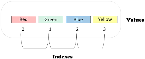
Figure 2.1: A four-element list in Python
Now, we will run the code:
bin_colors[1]'Green'Note that Python is a zero-indexing language. This means that the initial index of any data structure, including lists, will be
0.Green, which is the second element, is retrieved by index1– that is,bin_colors[1].
- List slicing: Retrieving a subset of the elements of a list by specifying a range of indexes is called slicing. The following code can be used to create a slice of the list:
bin_colors[0:2]['Red', 'Green']Note that lists are one of the most popular single-dimensional data structures in Python.
While slicing a list, the range is indicated as follows: the first number (inclusive) and the second number (exclusive). For example,
bin_colors[0:2]will includebin_color[0]andbin_color[1]but notbin_color[2]. While using lists, this should be kept in mind, as some users of the Python language complain that this is not very intuitive.Let’s have a look at the following code snippet:
bin_colors=['Red','Green','Blue','Yellow']
bin_colors[2:]
['Blue', 'Yellow']bin_colors[:2]['Red', 'Green']If the starting index is not specified, it means the beginning of the list, and if the ending index is not specified, it means the end of the list, as demonstrated by the preceding code.
- Negative indexing: In Python, we also have negative indices, which count from the end of the list. This is demonstrated in the following code:
bin_colors=['Red','Green','Blue','Yellow']
bin_colors[:-1]
['Red', 'Green', 'Blue']bin_colors[:-2]['Red', 'Green']bin_colors[-2:-1]['Blue']Note that negative indices are especially useful when we want to use the last element as a reference point instead of the first one.
- Nesting: An element of a list can be of any data type. This allows nesting in lists. For iterative and recursive algorithms, this provides important capabilities.
Let’s have a look at the following code, which is an example of a list within a list (nesting):
a = [1,2,[100,200,300],6] max(a[2])300a[2][1]200
- Iteration: Python allows iterating over each element on a list by using a
forloop. This is demonstrated in the following example:for color_a in bin_colors: print(color_a + " Square")Red Square Green Square Blue Square Yellow Square
Note that the preceding code iterates through the list and prints each element. Now let us remove the last element from the stack using pop() function.
Modifying lists: append and pop operations
Let’s take a look at modifying some lists, including the append and pop operations.
Adding elements with append()
When you want to insert a new item at the end of a list, you employ the append() method. It works by adding the new element to the nearest available memory slot. If the list is already at full capacity, Python extends the memory allocation, replicates the previous items in this newly carved out space, and then slots in the new addition:
bin_colors = ['Red', 'Green', 'Blue', 'Yellow']
bin_colors.append('Purple')
print(bin_colors)
['Red', 'Green', 'Blue', 'Yellow', 'Purple']
Removing elements with pop()
To extract an element from the list, particularly the last one, the pop() method is a handy tool. When invoked, this method extracts the specified item (or the last item if no index is given). The elements situated after the popped item get repositioned to maintain memory continuity:
bin_colors.pop()
print(bin_colors)
['Red', 'Green', 'Blue', 'Yellow']
The range() function
The range() function can be used to easily generate a large list of numbers. It is used to auto-populate sequences of numbers in a list.
The range() function is simple to use. We can use it by just specifying the number of elements we want in the list. By default, it starts from zero and increments by one:
x = range(4)
for n in x:
  print(n)
0 1 2 3
We can also specify the end number and the step:
odd_num = range(3,30,2)
for n in odd_num:
  print(n)
3 5 7 9 11 13 15 17 19 21 23 25 27 29
The preceding range function will give us odd numbers from 3 to 29.
To iterate through a list, we can use the for function:
for i in odd_num:
    print(i*100)
300 500 700 900 1100 1300 1500 1700 1900 2100 2300 2500 2700 2900
We can use the range() function to generate a list of random numbers. For example, to simulate ten trials of a dice, we can use the following code:
import random
dice_output = [random.randint(1, 6) for x in range(10)]
print(dice_output)
[6, 6, 6, 6, 2, 4, 6, 5, 1, 4]
The time complexity of lists
The time complexity of various functions of a list can be summarized as follows using the Big O notation:
- Inserting an element: The insertion of an element at the end of a list typically has a constant time complexity, denoted as O(1). This means the time taken for this operation remains fairly consistent, irrespective of the list’s size.
- Deleting an element: Deleting an element from a list can have a time complexity of O(n) in its worst-case scenario. This is because, in the least favorable situation, the program might need to traverse the entire list before removing the desired element.
- Slicing: When we slice a list or extract a portion of it, the operation can take time proportional to the size of the slice; hence, its time complexity is O(n).
- Element retrieval: Finding an element within a list, without any indexing, can require scanning through all its elements in the worst case. Thus, its time complexity is also O(n).
- Copying: Creating a copy of the list necessitates visiting every element once, leading to a time complexity of O(n).
Tuples
The second data structure that can be used to store a collection is a tuple. In contrast to lists, tuples are immutable (read-only) data structures. Tuples consist of several elements surrounded by ( ).
Like lists, elements within a tuple can be of different types. They also allow their elements to be complex data types. So, there can be a tuple within a tuple providing a way to create a nested data structure. The capability to create nested data structures is especially useful in iterative and recursive algorithms.
The following code demonstrates how to create tuples:
bin_colors=('Red','Green','Blue','Yellow')
print(f"The second element of the tuple is {bin_colors[1]}")
The second element of the tuple is Green
print(f"The elements after third element onwards are {bin_colors[2:]}")
The elements after third element onwards are ('Blue', 'Yellow')
# Nested Tuple Data structure
nested_tuple = (1,2,(100,200,300),6)
print(f"The maximum value of the inner tuple {max(nested_tuple[2])}")
The maximum value of the inner tuple 300
Wherever possible, immutable data structures (such as tuples) should be preferred over mutable data structures (such as lists) due to performance. Especially when dealing with big data, immutable data structures are considerably faster than mutable ones. When a data structure is passed to a function as immutable, its copy does not need to be created as the function cannot change it. So, the output can refer to the input data structure. This is called referential transparency and improves the performance. There is a price we pay for the ability to change data elements in lists and we should carefully analyze whether it is really needed so we can implement the code as read-only tuples, which will be much faster.
Note that, as Python is a zero-index-based language, a[2] refers to the third element, which is a tuple, (100,200,300), and a[2][1] refers to the second element within this tuple, which is 200.
The time complexity of tuples
The time complexity of various functions of tuples can be summarized as follows (using Big O notation):
- Accessing an element: Tuples allow direct access to their elements via indexing. This operation is constant time, O(1), meaning the time taken remains consistent regardless of the tuple’s size.
- Slicing: When a portion of a tuple is extracted or sliced, the operation’s efficiency is proportional to the size of the slice, resulting in a time complexity of O(n).
- Element retrieval: Searching for an element in a tuple, in the absence of any indexing aid, might require traversing all its elements in the worst-case scenario. Hence, its time complexity is O(n).
- Copying: Duplicating a tuple, or creating its copy, requires iterating through each element once, giving it a time complexity of O(n).
Dictionaries and sets
In this section, we will discuss sets and dictionaries, which are used to store data in which there is no explicit or implicit ordering. Both dictionaries and sets are quite similar. The difference is that a dictionary has a key-value pair. A set can be thought of as a collection of unique keys.
Let us look into them one by one.
Dictionaries
Holding data as key-value pairs is important, especially in distributed algorithms. In Python, a collection of these key-value pairs is stored as a data structure called a dictionary. To create a dictionary, a key should be chosen as an attribute that is best suited to identify data throughout data processing. The limitation on the value of keys is that they must be hashable types. A hashable is the type of object on which we can run the hash function, generating a hash code that never changes during its lifetime. This ensures that the keys are unique and searching for a key is fast. Numeric types and flat immutable types are all hashable and are good choices for the dictionary keys. The value can be an element of any type, for example, a number or string. Python also always uses complex data types such as lists as values. Nested dictionaries can be created by using a dictionary as the data type of a value.
To create a simple dictionary that assigns colors to various variables, the key-value pairs need to be enclosed in { }. For example, the following code creates a simple dictionary consisting of three key-value pairs:
bin_colors ={
  "manual_color": "Yellow",
  "approved_color": "Green",
  "refused_color": "Red"
}
print(bin_colors)
{'manual_color': 'Yellow', 'approved_color': 'Green', 'refused_color': 'Red'}
The three key-value pairs created by the preceding piece of code are also illustrated in the following screenshot:
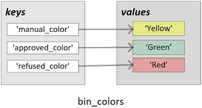
Figure 2.2: Key-value pairs in a simple dictionary
Now, let’s see how to retrieve and update a value associated with a key:
- To retrieve a value associated with a key, either the
getfunction can be used or the key can be used as the index:bin_colors.get('approved_color')'Green'bin_colors['approved_color']'Green' - To update a value associated with a key, use the following code:
bin_colors['approved_color']="Purple"
print(bin_colors)
{'manual_color': 'Yellow', 'approved_color': 'Purple', 'refused_color': 'Red'}
Note that the preceding code shows how we can update a value related to a particular key in a dictionary.
When iterating through a dictionary, usually, we will need both the keys and the values. We can iterate through a dictionary in Python by using .items():
for k,v in bin_colors.items():
    print(k,'->',v+' color')
manual_color -> Yellow color
approved_color -> Purple color
refused_color -> Red color
To del an element from a dictionary, we will use the del function:
del bin_colors['approved_color']
print(bin_colors)
{'manual_color': 'Yellow', 'refused_color': 'Red'}
The time complexity of a dictionary
For Python dictionaries, the time complexities for various operations are listed here:
- Accessing a value by key: Dictionaries are designed for fast look-ups. When you have the key, accessing the corresponding value is, on average, a constant time operation, O(1). This holds true unless there’s a hash collision, which is a rare scenario.
- Inserting a key-value pair: Adding a new key-value pair is generally a swift operation with a time complexity of O(1).
- Deleting a key-value pair: Removing an entry from a dictionary, when the key is known, is also an O(1) operation on average.
- Searching for a key: Verifying the presence of a key, thanks to hashing mechanisms, is usually a constant time, O(1), operation. However, worst-case scenarios could elevate this to O(n), especially with many hash collisions.
- Copying: Creating a duplicate of a dictionary necessitates going through each key-value pair, resulting in a linear time complexity, O(n).
Sets
Closely related to a dictionary is a set, which is defined as an unordered collection of distinct elements that can be of different types. One of the ways to define a set is to enclose the values in { }. For example, have a look at the following code block:
green = {'grass', 'leaves'}
print(green)
{'leaves', 'grass'}
The defining characteristic of a set is that it only stores the distinct value of each element. If we try to add another redundant element, it will ignore that, as illustrated in the following:
green = {'grass', 'leaves','leaves'}
print(green)
{'leaves', 'grass'}
To demonstrate what sort of operations can be done on sets, let’s define two sets:
- A set named
yellow, which has things that are yellow - A set named
red, which has things that are red
Note that some things are common between these two sets. The two sets and their relationship can be represented with the help of the following Venn diagram:
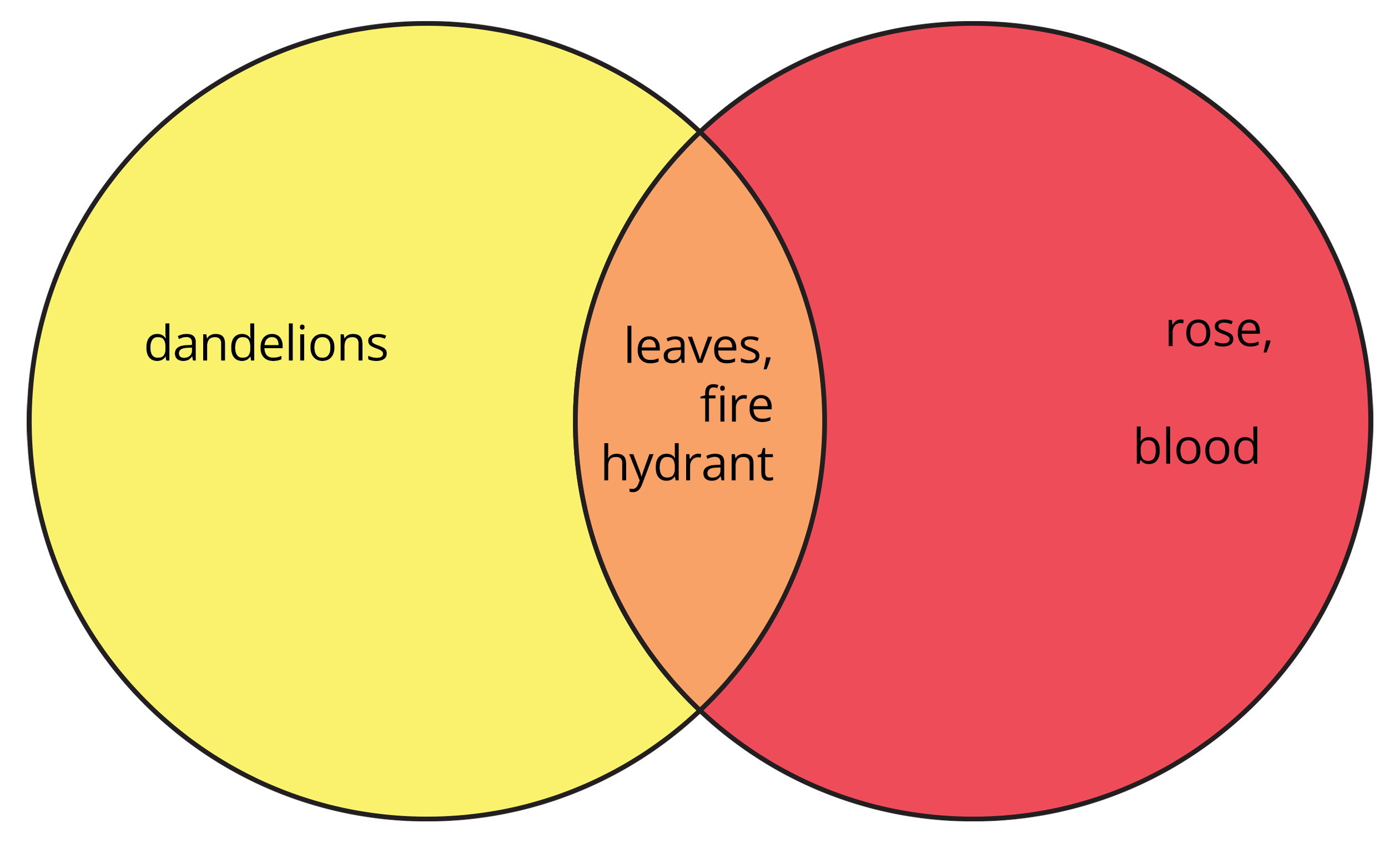
Figure 2.3: Venn diagram showing how elements are stored in sets
If we want to implement these two sets in Python, the code will look like this:
yellow = {'dandelions', 'fire hydrant', 'leaves'}
red = {'fire hydrant', 'blood', 'rose', 'leaves'}
Now, let’s consider the following code, which demonstrates set operations using Python:
print(f"The union of yellow and red sets is {yellow|red}")
The union of yellow and red sets is {leaves, blood, dandelions, fire hydrant, rose}
print(f"The intersection of yellow and red is {yellow&red}")
The intersection of yellow and red is {'fire hydrant', 'leaves'}
As shown in the preceding code snippet, sets in Python can have operations such as unions and intersections. As we know, a union operation combines all of the elements of both sets, and the intersection operation will give a set of common elements between the two sets. Note the following:
yellow|redis used to get the union of the preceding two defined sets.yellow&redis used to get the overlap between yellow and red.
As sets are unordered, the items of a set have no index. That means that we cannot access the items by referring to an index.
We can loop through the set items using a for loop:
for x in yellow:
    print(x)
fire hydrant
leaves
dandelions
We can also check if a specified value is present in a set by using the in keyword.
print("leaves" in yellow)
True
Time complexity analysis for sets
The following is the time complexity analysis for sets:
|
Sets |
Complexity |
|
Add an element |
|
|
Remove an element |
|
|
Copy |
|
Table 2.2: Time complexity for sets
When to use a dictionary and when to use a set
Let us assume that we are looking for a data structure for our phone book. We want to store the phone numbers of the employees of a company. For this purpose, a dictionary is the right data structure. The name of each employee will be the key and the value will be the phone number:
employees_dict = {
    "Ikrema Hamza": "555-555-5555",
    "Joyce Doston" : "212-555-5555",
}
But if we want to store only the unique value of the employees, then that should be done using sets:
employees_set = {
    "Ikrema Hamza",
    "Joyce Doston"
}
Using Series and DataFrames
Processing data is one of the core things that need to be done while implementing most of the algorithms. In Python, data processing is usually done by using various functions and data structures of the pandas library.
In this section, we will look into the following two important data structures of the pandas library, which will be used to implement various algorithms later in this book:
- Series: A one-dimensional array of values
- DataFrame: A two-dimensional data structure used to store tabular data
Let us look into the Series data structure first.
Series
In the pandas library, a Series is a one-dimensional array of values for homogenous data. We can think of a Series as a single column in a spreadsheet. We can think of Series as holding various values of a particular variable.
A Series can be defined as follows:
import pandas as pd
person_1 = pd.Series(['John',"Male",33,True])
print(person_1)
0    John
1    Male
2    33
3    True
dtype:    object
Note that in pandas Series-based data structures, there is a term called “axis,” which is used to represent a sequence of values in a particular dimension. Series has only “axis 0” because it has only one dimension. We will see how this axis concept is applied to a DataFrame in the next section.
DataFrame
A DataFrame is built upon the Series data structure. It is stored as two-dimensional tabular data. It is used to process traditional structured data. Let’s consider the following table:
|
id |
name |
age |
decision |
|
1 |
Fares |
32 |
True |
|
2 |
Elena |
23 |
False |
|
3 |
Doug |
40 |
True |
Now, let’s represent this using a DataFrame.
A simple DataFrame can be created by using the following code:
employees_df = pd.DataFrame([
    ['1', 'Fares', 32, True],
    ['2', 'Elena', 23, False],
    ['3', 'Doug', 40, True]])
employees_df.columns = ['id', 'name', 'age', 'decision']
print(employees_df)
    id    name    age    decision
0    1    Fares    32    True
1    2    Elena    23    False
2    3    Doug    40    True
Note that, in the preceding code, df.column is a list that specifies the names of the columns. In DataFrame, a single column or row is called an axis.
DataFrames are also used in other popular languages and frameworks to implement a tabular data structure. Examples are R and the Apache Spark framework.
Creating a subset of a DataFrame
Fundamentally, there are two main ways of creating the subset of a DataFrame:
- Column selection
- Row selection
Let’s look at them one by one.
Column selection
In machine learning algorithms, selecting the right set of features is an important task. Out of all of the features that we may have, not all of them may be needed at a particular stage of the algorithm. In Python, feature selection is achieved by column selection, which is explained in this section.
A column may be retrieved by name, as in the following:
df[['name','age']]
     name    age
0    Fares    32
1    Elena    23
2    Doug     40
The positioning of a column is deterministic in a DataFrame. A column can be retrieved by its position, as follows:
df.iloc[:,3]
0    True
1    False
2    True
Name: decision, dtype: bool
Note that, in this code, we are retrieving all rows of the DataFrame.
Row selection
Each row in a DataFrame corresponds to a data point in our problem space. We need to perform row selection if we want to create a subset of the data elements that we have in our problem space. This subset can be created by using one of the two following methods:
- By specifying their position
- By specifying a filter
A subset of rows can be retrieved by its position, as follows:
df.iloc[1:3,:]
    id    name    age    decision
1    2    Elena    23    False
Note that the preceding code will return the second and third rows plus all columns. It uses the iloc method, which allows us to access the elements by their numerical index.
To create a subset by specifying the filter, we need to use one or more columns to define the selection criterion. For example, a subset of data elements can be selected by this method, as follows:
df[df.age>30]
    id    name    age    decision
0    1    Fares    32    True
2    3    Doug     40    True
df[(df.age<35)&(df.decision==True)] id name age decision
    id    name    age    decision
0    1    Fares    32    True
Note that this code creates a subset of rows that satisfies the condition stipulated in the filter.
Time complexity analysis for sets
Let’s unveil the time complexities of some fundamental DataFrame operations.
- Selection operations
- Column selection: Accessing a DataFrame column, often done using the bracket notation or dot notation (for column names without spaces), is an O(1) operation. It offers a quick reference to the data without copying.
- Row selection: Using methods like
.loc[]or.iloc[]to select rows, especially with slicing, has a time complexity of O(n), where “n” represents the number of rows you’re accessing.
- Insertion operations
- Column insertion: Appending a new column to a DataFrame is typically an O(1) operation. However, the actual time can vary depending on the data type and size of the data being added.
- Row insertion: Adding rows using methods like
.append()or.concat()can result in an O(n) complexity since it often requires rearranging and reallocation.
- Deletion operations
- Column deletion: Dropping a column from a DataFrame, facilitated by the
.drop()method, is an O(1) operation. It marks the column for garbage collection rather than immediate deletion. - Row deletion: Similar to row insertion, row deletion can lead to an O(n) time complexity, as the DataFrame has to rearrange its structure.
- Column deletion: Dropping a column from a DataFrame, facilitated by the
Matrices
A matrix is a two-dimensional data structure with a fixed number of columns and rows. Each element of a matrix can be referred to by its column and the row.
In Python, a matrix can be created by using a numpy array or a list. But numpy arrays are much faster than lists because they are collections of homogenous data elements located in a contiguous memory location. The following code can be used to create a matrix from a numpy array:
import numpy as np
matrix_1 = np.array([[11, 12, 13], [21, 22, 23], [31, 32, 33]])
print(matrix_1)
[[11 12 13]
 [21 22 23]
 [31 32 33]]
print(type(matrix_1))
<class 'numpy.ndarray'>
Note that the preceding code will create a matrix that has three rows and three columns.
Matrix operations
There are many operations available for matrix data manipulation. For example, let’s try to transpose the preceding matrix. We will use the transpose() function, which will convert columns into rows and rows into columns:
print(matrix_1.transpose())
array([[11, 21, 31],
       [12, 22, 32],
       [13, 23, 33]])
Note that matrix operations are used a lot in multimedia data manipulation.
Big O notation and matrices
When discussing the efficiency of operations, the Big O notation provides a high-level understanding of its impact as data scales:
- Access: Accessing an element, whether in a Python list or a
numpyarray, is a constant time operation, O(1). This is because, with the index of the element, you can directly access it. - Appending: Appending an element at the end of a Python list is an average-case O(1) operation. However, for a numpy array, the operation can be O(n) in the worst case, as the entire array might need to be copied to a new memory location if there’s no contiguous space available.
- Matrix multiplication: This is where numpy shines. Matrix multiplication can be computationally intensive. Traditional methods can have a time complexity of O(n3) for n x n matrices. However,
numpyuses optimized algorithms, like the Strassen algorithm, which reduces this significantly.
Now that we have learned about data structures in Python, let’s move on to abstract data types in the next section.
Exploring abstract data types
Abstract data types (ADTs) are high-level abstractions whose behavior is defined by a set of variables and a set of related operations. ADTs define the implementation guidance of “what” needs to be expected but give the programmer freedom in “how” it will be exactly implemented. Examples are vectors, queues, and stacks. This means that two different programmers can take two different approaches to implementing an ADT, like a stack. By hiding the implementation level details and giving the user a generic, implementation-independent data structure, the use of ADTs creates algorithms that result in simpler and cleaner code. ADTs can be implemented in any programming language, such as C++, Java, and Scala. In this section, we shall implement ADTs using Python. Let’s start with vectors first.
Vector
A vector is a single-dimension structure for storing data. They are one of the most popular data structures in Python. There are two ways of creating vectors in Python, as follows:
- Using a Python list: The simplest way to create a vector is by using a Python list, as follows:
vector_1 = [22,33,44,55]
print(vector_1)
[22, 33, 44, 55]print(type(vector_1))<class 'list'>
Note that this code will create a list with four elements.
- Using a numpy array: Another popular way to create a vector is to use
numpyarrays.numpyarrays are generally faster and more memory-efficient than Python lists, especially for operations that involve large amounts of data. This is becausenumpyis designed to work with homogenous data and can take advantage of low-level optimizations. Anumpyarray can be implemented as follows:vector_2 = np.array([22,33,44,55]) print(vector_2)[22 33 44 55]print(type(vector_2))<class 'numpy.ndarray'>
Note that we created myVector using np.array in this code.
In Python, we can represent integers using underscores to separate parts. This makes them more readable and less error-prone. This is especially useful when dealing with large numbers. So, one billion can be represented as 1000_000_000.
large_number=1000_000_000
print(large_number)
1000000000
Time complexity of vectors
When discussing the efficiency of vector operations, it’s vital to understand the time complexity:
- Access: Accessing an element in both a Python list and a
numpyarray (vector) takes constant time, O(1). This ensures rapid data retrieval. - Appending: Appending an element to a Python list has an average time complexity of O(1). However, for a numpy array, appending could take up to O(n) in the worst case since numpy arrays require contiguous memory locations.
- Searching: Finding an element in a vector has a time complexity of O(n) because, in the worst case, you might have to scan through all elements.
Stacks
A stack is a linear data structure to store a one-dimensional list. It can store items either in a Last-In, First-Out (LIFO) or First-In, Last-Out (FILO) manner. The defining characteristic of a stack is the way elements are added to and removed from it. A new element is added at one end and an element is removed from that end only.
The following are the operations related to stacks:
- isEmpty: Returns
trueif the stack is empty - push: Adds a new element
- pop: Returns the element added most recently and removes it
Figure 2.4 shows how push and pop operations can be used to add and remove data from a stack:
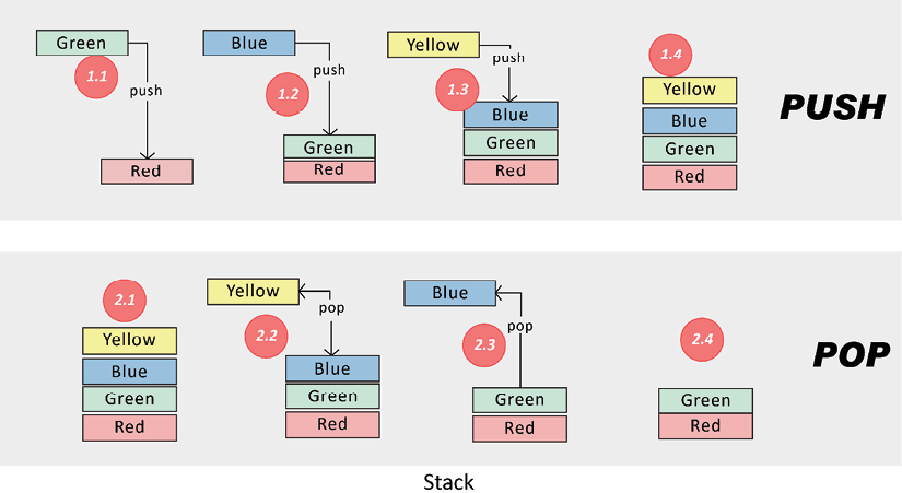
Figure 2.4: Push and pop operations
The top portion of Figure 2.4 shows the use of push operations to add items to the stack. In steps 1.1, 1.2, and 1.3, push operations are used three times to add three elements to the stack. The bottom portion of the preceding diagram is used to retrieve the stored values from the stack. In steps 2.2 and 2.3, pop operations are used to retrieve two elements from the stack in LIFO format.
Let’s create a class named Stack in Python, where we will define all of the operations related to the Stack class. The code of this class will be as follows:
class Stack:
     def __init__(self):
         self.items = []
     def isEmpty(self):
         return self.items == []
     def push(self, item):
         self.items.append(item)
     def pop(self):
         return self.items.pop()
     def peek(self):
         return self.items[len(self.items)-1]
     def size(self):
         return len(self.items)
To push four elements to the stack, the following code can be used:
Populate the stack
stack=Stack()
stack.push('Red')
stack.push('Green')
stack.push("Blue")
stack.push("Yellow")
Note that the preceding code creates a stack with four data elements:
Pop
stack.pop()
stack.isEmpty()
Time complexity of stack operations
Let us look into the time complexity of stack operations:
- Push: This operation adds an element to the top of the stack. Since it doesn’t involve any iteration or checking, the time complexity of the push operation is O(1), or constant time. The element is placed on top regardless of the stack’s size.
- Pop: Popping refers to removing the top element from the stack. Given that there’s no need to interact with the rest of the stack, the pop operation also has a time complexity of O(1). It’s a direct action on the top element.
Practical example
A stack is used as the data structure in many use cases. For example, when a user wants to browse the history in a web browser, it is a LIFO data access pattern, and a stack can be used to store the history. Another example is when a user wants to perform an undo operation in word processing software.
Queues
Like stacks, a queue stores n elements in a single-dimensional structure. The elements are added and removed in FIFO format. One end of the queue is called the rear and the other is called the front. When elements are removed from the front, the operation is called dequeue. When elements are added at the rear, the operation is called enqueue.
In the following diagram, the top portion shows the enqueue operation. Steps 1.1, 1.2, and 1.3 add three elements to the queue and the resultant queue is shown in 1.4. Note that Yellow is the rear and Red is the front.
The bottom portion of the following diagram shows a dequeue operation. Steps 2.2, 2.3, and 2.4 remove elements from the queue one by one from the front of the queue:
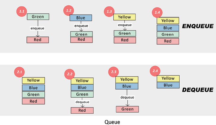
Figure 2.5: Enqueue and dequeue operations
The queue shown in the preceding diagram can be implemented by using the following code:
class Queue(object):
   def __init__(self):
      self.items = []
   def isEmpty(self):
      return self.items == []
   def enqueue(self, item):
       self.items.insert(0,item)
   def dequeue(self):
      return self.items.pop()
   def size(self):
      return len(self.items)
Let’s enqueue and dequeue elements as shown in the preceding diagramm with the help of the following code:
# Using Queue
queue = Queue()
queue.enqueue("Red")
queue.enqueue('Green')
queue.enqueue('Blue')
queue.enqueue('Yellow')
print(f"Size of queue is {queue.size()}")
Size of queue is 4
print(queue.dequeue())
Red
Note that the preceding code creates a queue first and then enqueues four items into it.
Time complexity analysis for queues
Let us look into the time complexity for queues:
- Enqueue: This operation inserts an element t the end of the queue. Given its straightforward nature, without any need for iterating or traversing, the
enqueueoperation bears a time complexity of O(1) – a constant time. - Dequeue: Dequeueing means removing the front element from the queue. As the operation only involves the first element without any checks or iterations through the queue, its time complexity remains constant at O(1).
The basic idea behind the use of stacks and queues
Let’s look into the basic idea behind the use of stacks and queues using an analogy. Let’s assume that we have a table where we put our incoming mail from our postal service, for example, Canada Mail. We stack them until we have some time to open and look at the letters, one by one. There are two possible ways of doing this:
- We put the letters in a stack and, whenever we get a new letter, we put it on the top of the stack. When we want to read a letter, we start with the one that is on top. This is what we call a stack. Note that the latest letter to arrive will be on the top and will be processed first. Picking up a letter from the top of the list is called a
popoperation. Whenever a new letter arrives, putting it on the top is called apushoperation. If we end up having a sizable stack and lots of letters are continuously arriving, there is a chance that we never get a chance to reach a very important letter waiting for us at the lower end of the stack. - We put the letters in the pile, but we want to handle the oldest letter first; every time we want to look at one or more letters, we take care to handle the oldest one first. This is what we call a queue. Adding a letter to the pile is called an
enqueueoperation. Removing the letter from the pile is called adequeueoperation.
Tree
In the context of algorithms, a tree is one of the most useful data structures due to its hierarchical data storage capabilities. While designing algorithms, we use trees wherever we need to represent hierarchical relationships among the data elements that we need to store or process.
Let’s look deeper into this interesting and quite important data structure.
Each tree has a finite set of nodes so that it has a starting data element called a root and a set of nodes joined together by links called branches.
Terminology
Let’s look into some of the terminology related to the tree data structure:
|
Root node |
A node with no parent is called the root node. For example, in the following diagram, the root node is A. In algorithms, usually, the root node holds the most important value in the tree structure. |
|
Level of a node |
The distance from the root node is the level of a node. For example, in the following diagram, the level of nodes D, E, and F is two. |
|
Siblings nodes |
Two nodes in a tree are called siblings if they are at the same level. For example, if we check the following diagram, nodes B and C are siblings. |
|
Child and parent node |
Node F is a child of node C if both are directly connected and the level of node C is less than node F. Conversely, node C is a parent of node F. Nodes C and F in the following diagram show this parent-child relationship. |
|
Degree of a node |
The degree of a node is the number of children it has. For example, in the following diagram, node B has a degree of two. |
|
Degree of a tree |
The degree of a tree is equal to the maximum degree that can be found among the constituent nodes of a tree. For example, the tree presented in the following diagram has a degree of two. |
|
Subtree |
A subtree of a tree is a portion of the tree with the chosen node as the root node of the subtree and all of the children as the nodes of the tree. For example, a subtree at node E of the tree presented in the following diagram consists of node E as the root node and nodes G and H as the two children. |
|
Leaf node |
A node in a tree with no children is called a leaf node. For example, in the following figure, nodes D, G, H, and F are the four leaf nodes. |
|
Internal node |
Any node that is neither a root nor a leaf node is an internal node. An internal node will have at least one parent and at least one child node. |
Note that trees are a kind of network or graph that we will study in Chapter 6, Unsupervised Machine Learning Algorithms. For graphs and network analysis, we use the terms link or edge instead of branches. Most of the other terminology remains unchanged.
Types of trees
There are different types of trees, which are explained as follows:
- Binary tree: If the degree of a tree is two, that tree is called a binary tree. For example, the tree shown in the following diagram is a binary tree as it has a degree of two:
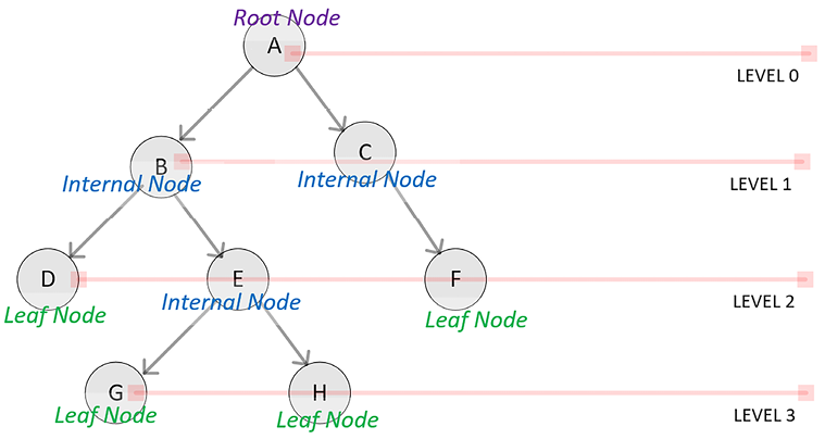
Figure 2.6: A binary tree
Note that the preceding diagram shows a tree that has four levels with eight nodes.
- Full tree: A full tree is one in which all of the nodes are of the same degree, which will be equal to the degree of the tree. The following diagram shows the kinds of trees discussed earlier:
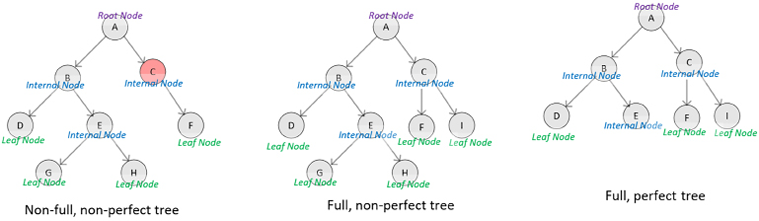
Figure 2.7: A full tree
Note that the binary tree on the left is not a full tree, as node C has a degree of one and all other nodes have a degree of two. The tree in the middle and the one on the right are both full trees.
- Perfect tree: A perfect tree is a special type of full tree in which all the leaf nodes are at the same level. For example, the binary tree on the right as shown in the preceding diagram is a perfect, full tree as all the leaf nodes are at the same level – that is, level 2.
- Ordered tree: If the children of a node are organized in some order according to particular criteria, the tree is called an ordered tree. A tree, for example, can be ordered from left to right in ascending order in which the nodes at the same level will increase in value while traversing from left to right.
Practical examples
An ADT tree is one of the main data structures that is used in developing decision trees, as will be discussed in Chapter 7, Traditional Supervised Learning Algorithms. Due to its hierarchical structure, it is also popular in algorithms related to network analysis, as will be discussed in detail in Chapter 6, Unsupervised Machine Learning Algorithms. Trees are also used in various search and sort algorithms in which divide and conquer strategies need to be implemented.
Summary
In this chapter, we discussed data structures that can be used to implement various types of algorithms. After going through this chapter, you should now be able to select the right data structure to be used to store and process data with an algorithm. You should also be able to understand the implications of our choice on the performance of the algorithm.
The next chapter is about sorting and searching algorithms, in which we will use some of the data structures presented in this chapter in the implementation of the algorithms.
Learn more on Discord
To join the Discord community for this book – where you can share feedback, ask questions to the author, and learn about new releases – follow the QR code below: