
10
Understanding Sequential Models
A sequence works in a way a collection never can.
—George Murray
This chapter covers an important class of machine learning models, the sequential models. A defining characteristic of such models is that the processing layers are arranged in such a way that the output of one layer is the input to the other. This architecture makes them perfect to process sequential data. Sequential data is the type of data that consists of ordered series of elements such as a sentence in a document or a time series of stock market prices.
In this chapter, we will start with understanding the characteristics of sequential data. Then, we will present the working of RNNs and how they can be used to process sequential data. Next, we will learn how we can address the limitations of RNN through GRU without scarifying accuracy. Then, we will discuss the architecture of LSTM. Finally, we will compare different sequential modeling architectures with a recommendation on when to use which one.
In this chapter, we will go through the following concepts:
- Understanding sequential data
- How RNNs can process sequential data
- Addressing the limitations of RNNs through GRUs
- Understanding LSTM
Let us start by first looking into the characteristics of sequential data.
Understanding sequential data
Sequential data is a specific type of data structure where the order of the elements matters, and each element has a relational dependency on its predecessors. This “sequential behavior” is distinct because it conveys information not just in the individual elements but also in the pattern or sequence in which they occur. In sequential data, the current observation is not only influenced by external factors but also by previous observations in the sequence. This dependency forms the core characteristic of sequential data.
Understanding the different types of sequential data is essential to appreciate its broad applications. Here are the primary categories:
- Time series data: This is a series of data points indexed or listed in time order. The value at any point in time is dependent on the past values. Time series data is widely used in various fields, including economics, finance, and healthcare.
- Textual data: Text data is also sequential in nature, where the order of words, sentences, or paragraphs can convey meaning. Natural language processing (NLP) leverages this sequential property to analyze and interpret human languages.
- Spatial-temporal data: This involves data that captures both spatial and temporal relationships, such as weather patterns or traffic flow over time in a specific geographical area.
Here’s how these types of sequential data manifest in real-world scenarios:
- Time series data: This type of data is clearly illustrated through financial market trends, where stock prices constantly vary in response to ongoing market dynamics. Similarly, sociological studies might analyze birth rates, reflecting year-to-year changes influenced by factors like economic conditions and social policies.
- Textual data: The sequential nature of text is paramount in literary and journalistic works. In novels, news articles, or essays, the specific ordering of words, sentences, and paragraphs constructs narratives and arguments, giving the text meaning beyond individual words.
- Spatial-temporal data: Areas in which this data type is vital are urban development and environmental studies. For instance, housing prices across different regions might be tracked over time to identify economic trends, while meteorological studies might monitor weather changes at specific geographical locations to forecast patterns and natural events.
These real-world examples demonstrate how the inherent sequential behavior in different types of data can be leveraged to provide insights and drive decisions across various domains.
In deep learning, handling sequential data requires specialized neural network architectures like sequential models. These models are designed to capture and exploit the temporal dependencies that inherently exist among the elements of sequential data. By recognizing these dependencies, sequential models provide a robust framework for creating more nuanced and effective machine learning models.
In summary, sequential data is a rich and complex type of data that finds applications across diverse domains. Recognizing its sequential nature, understanding its types, and leveraging specialized models enable data scientists to draw deeper insights and build more powerful predictive tools. Before we study the technical details, let us start by looking at the history of sequential modeling techniques.
Let us study different types of sequential models.
Types of sequence models
Sequential models are classified into various categories by examining the kind of data they handle, both in terms of input and output. This classification takes into account the specific nature of the data being used (like textual information, numerical data, or time-based patterns), and also how this data evolves or transforms from the beginning of the process to the end. By delving into these characteristics, we can identify three principal types of sequence models.
One-to-many
In one-to-many sequence models, a singular event or input can initiate the generation of an entire sequence. This unique attribute opens doors to a wide range of applications, but it also leads to complexities in training and implementation. The one-to-many sequence models offer exciting opportunities but come with inherent complexities in training and execution. As generative AI continues to advance, these models are likely to play a pivotal role in shaping creative and customized solutions across various domains.
The key to harnessing their potential lies in understanding their capabilities and recognizing the intricacies of training and implementation. The one-to-many sequence model is shown in Figure 10.1:
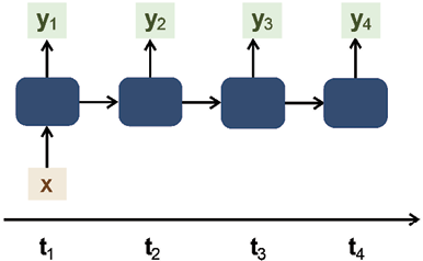
Figure 10.1: One-to-many sequential model
Let’s delve into the characteristics, capabilities, and challenges of one-to-many models:
- Wide range of applications: The ability to translate a single input into a meaningful sequence makes one-to-many models versatile and powerful. They can be employed to write poetry, create art such as drawings and paintings, and even craft personalized cover letters for job applications.
- Part of generative AI: These models fall under the umbrella of generative AI, a burgeoning field that aims to create new content that is both coherent and contextually relevant. This is what allows them to perform such varied tasks as mentioned above.
- Intensive training process: Training one-to-many models is typically more time-consuming and computationally expensive compared to other sequence models. The reason for this lies in the complexity of translating a single input into a wide array of potential outputs. The model must learn not only the relationship between the input and the output but also the intricate patterns and structures inherent in the generated sequence.
Note that unlike one-to-one models, where a single input corresponds to a single output, or many-to-many models, where a sequence of inputs is mapped to a sequence of outputs, the one-to-many paradigm must learn to extrapolate a rich and structured sequence from a singular starting point. This requires a deeper understanding of the underlying patterns and can often necessitate more sophisticated training algorithms.
The one-to-many approach isn’t without its challenges. Ensuring that the generated sequence maintains coherence, relevance, and creativity requires careful design and fine-tuning. It often demands a more extensive dataset and expert knowledge in the specific domain to guide the model’s training.
Many-to-one
Many-to-one sequential models are specialized tools in data analysis that take a sequence of inputs and convert them into a single output. This process of synthesizing multiple inputs into one concise output forms the core of the many-to-one model, allowing it to distill the essential characteristics of the data.
These models have diverse applications, such as in sentiment analysis, where a sequence of words like a review or a post is analyzed to determine an overall sentiment such as positive, negative, or neutral. The many-to-one sequential model is shown in Figure 10.2:
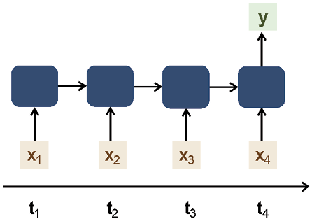
Figure 10.2: Many-to-one sequential model
The training process of many-to-one models is a complex yet integral part of their functionality. It distinguishes them from one-to-many models, whose focus is on creating a sequence from a single input. In contrast, many-to-one models must efficiently compress information, demanding careful selection of algorithms and precise tuning of parameters.
Training a many-to-one model involves teaching it to identify the vital features of the input sequence and to represent them accurately in the output. This involves discarding irrelevant information, a task that requires intricate balancing. The training process also often necessitates specialized pre-processing and feature engineering, tailored to the specific nature of the input data.
As discussed in the prior subsection, the training of many-to-one models may be more challenging than other types, requiring a deeper understanding of the underlying relationships in the data. Continuous monitoring of the model’s performance during training, along with a methodical selection of data and hyperparameters, is essential for the success of the model.
Many-to-one models are noteworthy for their ability to simplify complex data into understandable insights, finding applications in various industries for tasks such as summarization, classification, and prediction. Although their design and training can be intricate, their unique ability to interpret sequential data provides inventive solutions to complex data analysis challenges.
Thus, many-to-one sequential models are vital instruments in contemporary data analysis, and understanding their particular training process is crucial for leveraging their capabilities fully. The training process, characterized by meticulous algorithm selection, parameter tuning, and domain expertise, sets these models apart. As the field progresses, many-to-one models will continue to offer valuable contributions to data interpretation and application.
Many-to-many
This is a type of sequential model that takes sequential data as the input, processes it in some way, and then generates sequential data as the output. An example of many-to-many models is machine translation, where a sequence of words in one language is translated into a corresponding sequence in another language. An illustrative example of this would be the translation of English text into French. While there are numerous machine translation models that fall into this category, a prominent approach is the use of Sequence-to-Sequence (Seq2Seq) models, particularly with STM networks. Seq2Seq models with LSTM have become a standard method for tasks such as English-to-French translation and have been implemented in various NLP frameworks and tools. The many-to-many sequential model is shown in Figure 10.3:
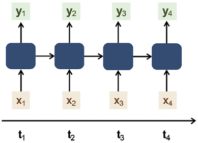
Figure 10.3: Many-to-many sequential model
Over the years, many algorithms have been developed to process and train machine learning models using sequential data. Let us start with studying how to represent sequential data with 3-dimensional data structures.
Data representation for sequential models
Timesteps add depth to the data, making it a 3D structure. In the context of sequential data, each “unit” or instance of this dimension is termed a “timestep.” This is crucial to remember: while the dimension is called “timesteps,” each individual data point in this dimension is a “timestep.” Figure 10.4 illustrates the three dimensions in data used for training RNNs, emphasizing the addition of timesteps:
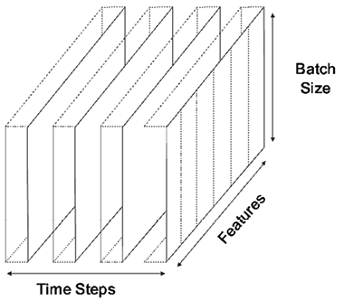
Figure 10.4: The 3D data structures used in RNN training
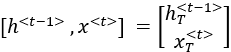
Given that the concept of timesteps is a new addition to our exploration, a special notation is introduced to represent it effectively. A superscript enclosing a timestep in angle brackets is paired with the variable in question. For example, using this notation, ![]() and
and ![]() represent the value of the variable
represent the value of the variable stock_price at timestep t1 and timestep t2, respectively.
The choice of dividing data into batches, essentially deciding the “length,” can be both an intentional design decision and influenced by external tools and libraries. Often, machine learning frameworks provide utilities to automatically batch data, but choosing an optimal batch size can be a combination of experimentation and domain knowledge.
Let us start the discussion on sequential modeling techniques with RNNs first.
Introducing RNNs
RNNs, are a special breed of neural networks designed specifically for sequential data. Here’s a breakdown of their key attributes.
The term “recurrent” stems from the unique feedback loop RNNs possess. Unlike traditional neural networks, which are essentially stateless and produce outputs solely based on the current inputs, RNNs carry forward a “state” from one step in the sequence to the next.
When we talk about a “run” in the context of RNNs, we’re referring to a single pass or processing of an element in the sequence. So, as the RNN processes each element, or each “run,” it retains some information from the previous steps.
The magic of RNNs lies in their ability to maintain a memory of previous runs or steps. They achieve this by incorporating an additional input, which is essentially the state or memory from the previous run. This mechanism allows RNNs to recognize and learn the dependencies between elements in a sequence, such as the relationships between consecutive words in a sentence.
Let us study the architecture of RNNs in detail.
Understanding the architecture of RNNs
First, let us define some variables:
 : the input at timestep t
 : actual output (ground truth) at timestep t
 : predicted output at timestep t
Understanding the memory cell and hidden state
RNNs stand out because of their inherent ability to remember and maintain context as they progress through different timesteps. This state at a certain timestep t is represented by ![]() , where h stands for hidden. It is the summary of the information learned up to a particular timestep. As shown in Figure 10.5, the RNN keeps on learning by updating its hidden state at each timestep. The RNN uses this hidden state at each timestep to keep a context. At its core, “context” refers to the collective information or knowledge an RNN retains from previous timesteps. It allows RNNs to memorize the state at each timestep and pass this information to the next timestep as it progresses along through the sequence. This hidden state makes the RNN stateful:
, where h stands for hidden. It is the summary of the information learned up to a particular timestep. As shown in Figure 10.5, the RNN keeps on learning by updating its hidden state at each timestep. The RNN uses this hidden state at each timestep to keep a context. At its core, “context” refers to the collective information or knowledge an RNN retains from previous timesteps. It allows RNNs to memorize the state at each timestep and pass this information to the next timestep as it progresses along through the sequence. This hidden state makes the RNN stateful:
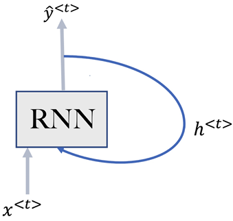
Figure 10.5: Hidden state in RNN
For example, if we use an RNN to translate a sentence from English to French, each input is a sentence that needs to be defined as sequential data. To get it right, the RNN cannot translate each word in isolation. It needs to capture the context of the words that have been translated so far, allowing the RNN to correctly translate the entire sentence. This is achieved through the hidden state that is calculated and stored at each timestep and passed on to the later ones.
The RNN’s strategy of memorizing the state with the intention of using it for future timesteps brings new research questions that need to be addressed. For example, what to remember and what to forget. And, perhaps the trickiest one, when to forget. The variants of RNN, like GRUs and LSTM, attempt to answer these questions in different ways.
Understanding the characteristics of the input variable
Let’s get a deeper understanding of the input variable, ![]() , and the methodology behind encoding it when working with RNNs. One of the pivotal applications for RNNs lies in the realm of NLP. Here, the sequential data we deal with comprises sentences. Think of each sentence as a sequence of words, such that a sentence can be delineated as:
, and the methodology behind encoding it when working with RNNs. One of the pivotal applications for RNNs lies in the realm of NLP. Here, the sequential data we deal with comprises sentences. Think of each sentence as a sequence of words, such that a sentence can be delineated as:
![]()
In this representation, ![]() denotes an individual word within the sentence. To avoid confusion: each
denotes an individual word within the sentence. To avoid confusion: each ![]() is not an entire sentence but rather an individual word within it.
is not an entire sentence but rather an individual word within it.
Each word, ![]() , is encoded using a one-hot vector. The length of this vector is defined by |V|, where:
, is encoded using a one-hot vector. The length of this vector is defined by |V|, where:
- V signifies our vocabulary set, which is a collection of distinct words.
- |V| quantifies the total number of entries in V.
In the context of widely-used applications, one could envision V as comprising the entire set of words found in a standard English dictionary, which may contain roughly 150,000 words. However, for specific NLP tasks, only a subset of this vast vocabulary is necessary.
Note: It’s essential to differentiate between V and |V|. While V stands for the vocabulary itself, |V| represents the size of this vocabulary.
When referring to the “dictionary,” we’re drawing from a general notion of standard English dictionaries. However, there are more exhaustive corpora available, like the Common Crawl, which can contain word sets stretching into the tens of millions.
For many applications, a subset of this vocabulary should be enough. Formally,
![]()
To understand the working of RNNs, let us examine the first timestep, t1.
Training the RNN at the first timestep
RNNs operate by analyzing sequences one timestep at a time. Let’s dive into the initial phase of this process. For the timestep t1, the network receives an input represented as ![]() . Based on this input, the RNN makes an initial prediction, which we denote as
. Based on this input, the RNN makes an initial prediction, which we denote as ![]() . At every timestep, tt, the RNN leverages the hidden state from the previous timestep,
. At every timestep, tt, the RNN leverages the hidden state from the previous timestep, ![]() , to provide contextual information.
, to provide contextual information.
However, at t1, since we’re just beginning, there’s no prior hidden state to reference. Therefore, the hidden state ![]() is initialized to zero.
is initialized to zero.
The activation function in action
Referencing Figure 10.6, you’ll notice an element marked by A. This represents the activation function, a crucial component in neural networks. Essentially, the activation function determines how much signal to pass onto the next layer. For this timestep, the activation function receives both the input ![]() and the previous hidden state
and the previous hidden state ![]() .
.
As discussed in Chapter 8, an activation function in neural networks is a mathematical equation that determines the output of a neuron based on its input. Its primary role is to introduce non-linearity into the network, enabling it to learn from errors and make adjustments, which is essential for learning complex patterns.
A recurring choice for the activation function in many neural networks is “tanh.” But what’s the reasoning behind this preference?
The world of neural networks isn’t without its challenges, and one such obstacle is the vanishing gradient problem. To put it plainly, as we keep training our model, occasionally, the gradient values, which guide our weight adjustments, diminish to tiny numbers. This drop means the changes we make to our network’s weights become almost negligible. Such minute tweaks result in an excruciatingly slow learning process, sometimes even coming to a standstill. Here’s where the “tanh" function shines. It’s chosen because it acts as a buffer against this vanishing gradient issue, steering the training process toward consistency and efficiency:
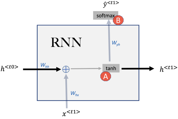
Figure 10.6: RNN training at timestep t1
As we zero in on the outcome of the activation function, we arrive at the value for the hidden state, ![]() . In mathematical terms, this relationship can be expressed as:
. In mathematical terms, this relationship can be expressed as:
![]()
This hidden state is not just a passing phase. It holds value as we step into the next timestep, t2. Think of it as a relay racer passing on the baton, or in this case, context, from one timestep to its successor, ensuring continuity in the sequence.
The second activation function (represented by B in Figure 10.7) is used to generate the predicted output ![]() at timestep t1. The choice of this activation function will depend on the type of the output variable. For instance, if an RNN is employed to predict stock market prices, the ReLU function can be adopted as the output variable is continuous. On the other hand, if we are doing sentiment analysis on a bunch of posts, it can be a sigmoid activation function. In Figure 10.7, assuming that it is a multiclass output variable, we are using the softmax activation function. Remember that a multiclass output variable refers to a situation where the output or the prediction can fall into one of several distinct classes. In machine learning, this is common in classification problems where the aim is to categorize an input into one of several predefined categories. For example, if we are categorizing objects as a car, bike, or bus, the output variable has multiple classes, thus is termed as “multiclass.” Mathematically, we can represent it as:
at timestep t1. The choice of this activation function will depend on the type of the output variable. For instance, if an RNN is employed to predict stock market prices, the ReLU function can be adopted as the output variable is continuous. On the other hand, if we are doing sentiment analysis on a bunch of posts, it can be a sigmoid activation function. In Figure 10.7, assuming that it is a multiclass output variable, we are using the softmax activation function. Remember that a multiclass output variable refers to a situation where the output or the prediction can fall into one of several distinct classes. In machine learning, this is common in classification problems where the aim is to categorize an input into one of several predefined categories. For example, if we are categorizing objects as a car, bike, or bus, the output variable has multiple classes, thus is termed as “multiclass.” Mathematically, we can represent it as:
![]()
From Eq. 10.1 and Eq. 10.2, It should be obvious that the objective of training the RNN is to find the optimal values of three sets of weight matrices (Whx, Whh, and Wyh) and two sets of biases (bh and by). As we progress, it becomes evident that these weights and biases maintain consistency across all timesteps.
Training the RNN for a whole sequence
Previously, we developed the mathematical formulation for the hidden state for the first timestep, t1. Let us now study the working of the RNN through more than one timestep to train a complete sequence, as shown in Figure 10.7:
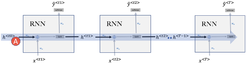
Figure 10.7: Sequential processing in RNN
Info: In Figure 10.7, it can be observed that the hidden state travels from left to right carrying the context forward shown by the arrow A. The ability of RNNs and their variants to create this “information highway” propagating through time is the defining feature of RNNs.
We calculated Eq. 10.1 for the timestep t1. For any timestep t, we can generalize Eq. 10.1 as:
![]()
For NLP applications, ![]() is encoded as a one-hot vector. In this case, the dimension of
is encoded as a one-hot vector. In this case, the dimension of ![]() will be equal to |V|, where V is the vector representing the vocabulary. The hidden variable
will be equal to |V|, where V is the vector representing the vocabulary. The hidden variable ![]() will be a lower-dimensional representation of the original input,
will be a lower-dimensional representation of the original input, ![]() . By lowering the dimension of the input variable
. By lowering the dimension of the input variable ![]() by many folds, we intend the hidden layer to capture only the important information of the input variable
by many folds, we intend the hidden layer to capture only the important information of the input variable ![]() . The dimension of
. The dimension of ![]() is represented by Dh.
is represented by Dh.
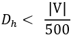
It is not unusual for ![]() to have dimensions 500 times lower than
to have dimensions 500 times lower than ![]() .
.
So, typically:
Because of the lower dimensions of ![]() , weight matrix Whh is a comparatively small data structure as
, weight matrix Whh is a comparatively small data structure as ![]() . Whx on the other hand, will be as wide as
. Whx on the other hand, will be as wide as ![]() .
.
Combining weight matrices
In Eq. 10.3, both Whh and Whx are used in the calculation of ![]() . To simplify the analysis, it helps to combine Whh and Whx into one weight parameter matrix,
. To simplify the analysis, it helps to combine Whh and Whx into one weight parameter matrix, ![]() . This simplified representation will be quite useful for the discussion of more complex variants of RNNs that are discussed later in this chapter.
. This simplified representation will be quite useful for the discussion of more complex variants of RNNs that are discussed later in this chapter.
To create one combined weight matrix, Wh, we simply horizontally concatenate Whh and Whx horizontally to create a combined weight matrix, Wh:
![]()
As we are simply horizontally concatenating, the dimensions of the Wh will have the same number of rows and total number of columns, i.e.,
![]()
Using Wh in Eq. 10.3:
![]()
Where ![]() indicates the vertical stacking of two vectors together.
indicates the vertical stacking of two vectors together.
Where ![]() and
and ![]() are the respective transposed vectors.
are the respective transposed vectors.
Let us look at a specific example.
Let us assume that we are using RNNs for an NLP application. The size of the vocabulary is 50,000 words. It means that each input ![]() will be encoded as a hot vector having a dimension of 50,000. Let assume that
will be encoded as a hot vector having a dimension of 50,000. Let assume that ![]() has a dimension of 50. It will be the lower-dimension representation of
has a dimension of 50. It will be the lower-dimension representation of ![]() .
.
Now, it should be obvious that Whh will have dimensions of (50![]() 50). Whx will have dimensions of (50
50). Whx will have dimensions of (50![]() 50,000).
50,000).
Going back to the above example, Wh will have dimensions of (50x50,000+50) = 50![]() 50,050, i.e.,:
50,050, i.e.,:
![]()
Calculating the output for each timestep
In our model, the output generated for a given timestep, such as t1, is denoted by ![]() . Since we are employing the softmax function for normalization in our model, the output for any timestep, tt, can be generalized using the following equation:
. Since we are employing the softmax function for normalization in our model, the output for any timestep, tt, can be generalized using the following equation:
![]()
Understanding how the output is calculated at each timestep lays the foundation for the subsequent stage of training, where we need to evaluate how well the model is performing.
Now that we have a grasp of how the outputs are generated at each timestep, it becomes essential to determine the discrepancy between these predicted outputs and the actual target values. This discrepancy, referred to as “loss,” gives us a measure of the model’s error. In the next section, we will delve into the methods of computing RNN loss, allowing us to gauge the model’s accuracy and make necessary adjustments to the weights and biases. This process is vital in training the model to make more accurate predictions, thereby enhancing its overall performance.
Computing RNN loss
As mentioned, the objective of training RNNs is to find the right values of three sets of weights (Whx, Whh, and Wyh) and two sets of biases (bh and by). Initially, at timestep t1, these values are initialized randomly.
As the training process progresses, these values are changed as the gradient descent algorithm kicks in. We need to compute loss at each timestep of the forward propagation in RNNs. Let us break down the process of computing the loss:
- Compute loss for individual timestep:
At timestep t1, the predicted output is
 . The expected output is
  . The actual loss function used will depend on the type of model we are training. For example, if we are training a classifier, then this loss at timestep t1 will be:
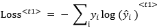
- Aggregate loss for complete sequence:
For a complete sequence consisting of multiple timesteps, we will compute the individual losses for each of the timesteps, {t1,t2,…tT). The loss for one sequence with T timesteps will be the aggregate of the loss of each timestep, as calculated by the following equation:

- Compute loss for multiple sequences in a batch:
If there is more than one sequence in the batch, then, first, the loss is calculated for each individual sequence. We then compute the cost across all the sequences in a particular batch and use it for backpropagation.
By calculating the loss in this structured manner, we guide the model in adjusting its weights and biases to better align with the desired output. This iterative process, repeated over many batches and epochs, allows the model to learn from the data and make more accurate predictions.
Backpropagation through time
Backpropagation, as explained in Chapter 8, is used in neural networks to progressively learn from the examples of training datasets. RNNs add another dimension to the training data, that is, the timesteps. Backpropagation through time (BPTT) is designed to handle the sequential data as the training process is going through the timesteps.
Backpropagation is triggered when the forward feed process calculates the loss of the last timestep of a batch. We then apply this derivative to adjust the weights and biases for the RNN model. RNNs have three sets of weights, Whh , Whx and Why, and two sets of biases (bh and by). Once the weights and biases are adjusted, we will continue with gradient descent for model training.
The name of this section, Backpropagation through time, does not hint toward any time machine that takes us back to some medieval era. Instead, it stems from the fact that once the cost has been calculated through forward-feed, it needs to run backward through each of the timesteps and update weights and biases.
The backpropagation process is crucial for tuning the model’s parameters, but once the model is trained, what’s next? After we’ve used backpropagation to minimize the loss, we have a model that’s ready to make predictions. In the next section, we’ll explore how to use the trained RNN model to make predictions on new data. We’ll find that predicting with RNNs is similar to the process used with fully connected neural networks, where the input data is processed by the trained RNN to produce the predictions. This shift from training to prediction forms a natural progression in understanding how RNNs can be applied to real-world problems.
Predicting with RNNs
Once the model is trained, predicting with RNNs is similar to with fully connected neural networks. The input data is given as input to the trained RNN model and predictions are obtained. Here’s how it functions:
- Input preparation: Just like in a standard neural network, you begin by preparing the input data. In the case of an RNN, this input data is typically sequential, representing timesteps in a process or series.
- Model utilization: You then feed this input data into the trained RNN model. The model’s learned weights and biases, optimized during the training phase, are used to process the input through each layer of the network. In an RNN, this includes passing the data through the recurrent connections that handle the sequential aspects of the data.
- Activation functions: As in other neural networks, activation functions within the RNN transform the data as it moves through the layers. Depending on the specific design of the RNN, different activation functions might be used at different stages.
- Generating predictions: The penultimate step is generating the predictions. The output of the RNN is processed through a final layer, often using a softmax activation function for classification tasks, to produce the final prediction for each input sequence.
- Interpretation: The predictions are then interpreted based on the specific task at hand. This could be classifying a sequence of text, predicting the next value in a time series, or any other task that relies on sequential data.
Thus, predicting with an RNN follows a process similar to that of fully connected neural networks, with the main distinction being the handling of sequential data. The RNN’s ability to capture temporal relationships within the data allows it to provide unique insights and predictions that other neural network architectures might struggle with.
Limitations of basic RNNs
Earlier in the chapter, we introduced basic RNNs. Sometimes we refer to basic RNNs as “plain vanilla” RNNs. This term refers to their fundamental, unadorned structure. While they serve as a solid introduction to recurrent neural networks, these basic RNNs do have notable limitations:
- Vanishing gradient problem: This issue makes it challenging for the RNN to learn and retain long-term dependencies in the data.
- Inability to look ahead in the sequence: Traditional RNNs process sequences from the beginning to the end, which limits their capability to understand the future context in a sequence.
Let us investigate them one by one.
Vanishing gradient problem
RNNs iteratively process the input data one timestep at a time. This means that as the input sequences become longer, RNNs find it hard to capture long-term dependencies. Long-term dependencies refer to relationships between elements in a sequence that are far apart from each other. Imagine analyzing a lengthy piece of text, such as a novel. If a character’s actions in the first chapter influence events in the last chapter, that’s a long-term dependency. The information from the beginning of the text has to be “remembered” all the way to the end for full understanding.
RNNs often struggle with such long-range connections. The hidden state mechanism of RNNs, designed to retain information from previous timesteps, can be too simplistic to capture these intricate relationships. As the distance between related elements grows, the RNN may lose track of the connection. There is not much intelligence on when and what to keep in memory and when and what to forget.
For many use cases in sequential data, only the most recent information is important. For example, consider a predictive text application trying to assist a person typing an email by suggesting the next word to type.
As we know, such functionality is now standard in modern word processors. If the user is typing:

Figure 10.8: Predictive text example
the predictive text application can easily suggest the next word “hard”. It does not need to bring the context from the prior sentences to predict the next word. For such applications, where long-term memory is not required, RNNs are the best choice. RNNs will not over-complicate the architecture without compromising on accuracy.
But for other applications, keeping the long-term dependencies is important. RNNs struggle with managing long-term dependencies. Let us look at an example:
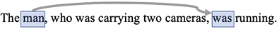
Figure 10.9: Predictive text example with a long-term dependency
As we read this sentence from left to right, we can observe that “was” (used later in the sentence) is referring to the “man.” RNNs in their original form will struggle to carry the hidden state forward for multiple timesteps. The reason is that, in RNNs, the hidden state is calculated for each timestep and carried forward.
Due to the recursive nature of this operation, we are always concerned about the signal prematurely fading while progressing from element to element in different timesteps. This behavior of RNNs is identified as the vanishing gradient problem. To combat this vanishing gradient problem, we prefer to choose tanh as the activation function. As the second derivative of tanh decays very slowly to zero, the choice of tanh helps manage the vanishing gradient problem to some extent. But we need more sophisticated architecture, like GRUs and LSTM, to better manage the vanishing gradient problem, which we will discuss in the next section.
Inability to look ahead in the sequence
RNNs can be categorized based on the direction of information flow through the sequence. The two primary types are unidirectional RNNs and bidirectional RNNs.
- Unidirectional RNNs: These networks process the input data in one direction, usually from the beginning of the sequence to the end. They carry the context forward, building understanding step by step as they iterate through the elements of a sequence, such as words in a sentence. Here’s the limitation: unidirectional RNNs cannot “look ahead” in the sequence.
They only have access to the information they’ve seen so far, meaning they can’t incorporate future elements to build a more accurate or nuanced context. Imagine reading a complex sentence one word at a time, without being able to glance ahead and see what’s coming. You might miss subtleties or misunderstand the overall meaning.
- Bidirectional RNNs: In contrast, bidirectional RNNs process the sequence in both directions simultaneously. They combine insights from both the past and the future elements, allowing for a richer understanding of the context.
Let us consider the following two sentences:
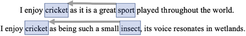
Figure 10.10: Examples where an RNN must look ahead in the sentence
Both of these sentences use the word “cricket.” If the context is built only from left to right, as done in unidirectional RNNs, we cannot contextualize “cricket” properly as its relevant information will be in a future timestep. To solve this problem, we will look into bidirectional RNNs, which are discussed in Chapter 11.11
Now let us study GRUs and their detailed working and architecture.
GRU
GRUs represent an evolution of the basic RNN structure, specifically designed to address some of the challenges encountered with traditional RNNs, such as the vanishing gradient problem. The architecture of a GRU is illustrated in Figure 10.8:
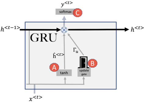
Figure 10.11: GRU
Let us start discussing GRU with the first activation function, annotated as A. At each timestep t, GRU first calculates the hidden state using the tanh activation function and utilizing ![]() and
and ![]() as inputs. The calculation is no different than how the hidden state is determined in the original RNNs presented in the previous section. But there is an important difference. The output is a candidate hidden state, which is calculated using Eq. 10.6:
as inputs. The calculation is no different than how the hidden state is determined in the original RNNs presented in the previous section. But there is an important difference. The output is a candidate hidden state, which is calculated using Eq. 10.6:
![]()
where ![]() is the candidate value of the hidden layer.
is the candidate value of the hidden layer.
Now, instead of using the candidate hidden state straight away, the GRU takes a moment to decide whether to use it. Imagine it like someone pausing to think before making a decision. This pause-and-think step is what we call the gating mechanism. It checks out the information and then selects what details to remember and what to forget for the next step. It’s kind of like filtering out the noise and focusing on the important stuff. By blending the old information (from the previous hidden state) and the new draft (the candidate), GRUs are better at following long stories or sequences without getting lost. By introducing a candidate hidden state, GRUs bring an added layer of flexibility. They can judiciously decide the portion of the candidate state to incorporate. This distinction equips GRUs to adeptly tackle challenges, such as the vanishing gradient, with a finesse that traditional RNNs often lack. In simpler terms, while the classic RNNs might struggle to remember long stories, GRUs, with their special features, are better listeners and retainers.
LSTM was proposed in 1997 and GRUs in 2014. Most books on this topic prefer the chronological order and present LSTMs first. I have chosen to present these algorithms ordered by complexity. As the motivation behind GRUs was to simplify LSTMs, it may be useful to study the simpler algorithm first.
Introducing the update gate
In a standard RNN, the hidden value at each timestep is calculated and automatically becomes the new state of the memory cell. In contrast, GRUs introduce a more nuanced approach. The GRU model brings more flexibility to the process by allowing control over when to update the state of the memory cell. This added flexibility is implemented through a mechanism called the “update gate,” sometimes referred to as the “reset gate.”
The update gate’s function is to evaluate whether the information in the candidate hidden state, ![]() , is significant enough to update the memory cell’s hidden state or if the memory cell should retain the old hidden value from previous timesteps.
, is significant enough to update the memory cell’s hidden state or if the memory cell should retain the old hidden value from previous timesteps.
In mathematical terms, this decision-making process helps the model to manage information more selectively, determining whether to integrate new insights or continue relying on previously acquired knowledge. If the model deems that the candidate hidden state’s information is not significant enough to alter the memory cell’s existing state, the previous hidden value will be retained. Conversely, if the new information is considered relevant, it can overwrite the memory cell’s state, thus adjusting the model’s internal representation as it processes the sequence.
This unique gating mechanism sets GRUs apart from traditional RNNs and allows for more effective learning from sequential data with complex temporal relationships.
Implementing the update gate
This intelligence that we add to how the state is updated in the memory cell is the defining feature of a GRU. The decision will be taken soon of whether we should update the current hidden state with the candidate hidden state. To make this decision, we use the second activation function shown in Figure 10.11, annotated as B. This activation function is implementing the update gate.
It is implemented as a sigmoid layer that takes as input the current input and the previous hidden state. The output of the sigmoid layer is a value between 0 and 1 represented by the variable ![]() The output of the update gate is the variable
The output of the update gate is the variable ![]() , which is governed by the following sigmoid function:
, which is governed by the following sigmoid function:
![]()
As ![]() is the output of a sigmoid function, it is close to either 1 or 0, which determines whether the update gate is open or closed. If the update gate is open,
is the output of a sigmoid function, it is close to either 1 or 0, which determines whether the update gate is open or closed. If the update gate is open, ![]() will be chosen as the new hidden
will be chosen as the new hidden state. In the training process, the GRU will learn when to open the gate and when to close it.
Updating the hidden cell
For a certain timestep, the next hidden state is determined using the calculation from the following equation:
![]()
Eq. 10.8 consists of two terms, annotated as 1 and 2. Being an output of a sigmoid function, ![]() can either be 0 or 1. It means:
can either be 0 or 1. It means:
![]()
![]()
In other words, if the gate is open, update the value of ![]() . Otherwise, just retain the old state.
. Otherwise, just retain the old state.
Let us now look into how we can run GRUs for multiple timesteps.
Running GRUs for multiple timesteps
When deploying GRUs across several timesteps, we can visualize this process as depicted in Figure 10.12. Much like the foundational RNNs we discussed in the prior segment, GRUs create what can be thought of as an “information highway.” This pathway effectively transfers context from the beginning to the end of a sequence, visualized as ![]() in Figure 10.12 and annotated as A.
in Figure 10.12 and annotated as A.
What differentiates GRUs from traditional RNNs is the decision-making process about how information flows on this highway. Instead of transferring information blindly at each timestep, a GRU pauses to evaluate its relevance.
Let’s illustrate this with a basic example. Imagine reading a book where each sentence is a piece of information. However, instead of remembering every detail about every sentence, your mind (acting like a GRU) selectively recalls the most impactful or emotional sentences. This selective memory is akin to how the update gate in a GRU works.
The update gate serves a crucial role here. It’s a mechanism that determines which portions of the prior information, or the prior “hidden state,” should be retained or discarded. Essentially, the gate helps the network zoom in on and retain the most pertinent details, ensuring that the carried context remains as relevant as possible.
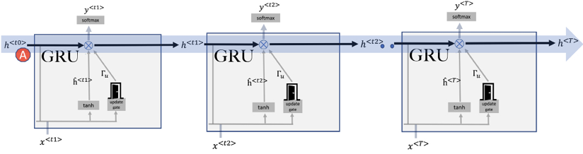
Figure 10.12: Sequential processing in RNN
Introducing LSTM
RNNs are widely used for sequence modeling tasks, but they suffer from limitations in capturing long-term dependencies in the data. An advanced version of RNNs, known as LSTM, was developed to address these limitations. Unlike simple RNNs, LSTMs have a more complex mechanism to manage context, enabling them to better capture patterns in sequences.
In the previous section, we discussed GRUs, where hidden state ![]() is used to carry the context from timestep to timestep. LSTM has a much more complex mechanism for managing the context. It has two variables that carry the context from timestep to timestep: the cell state and the hidden state. They are explained as follows:
is used to carry the context from timestep to timestep. LSTM has a much more complex mechanism for managing the context. It has two variables that carry the context from timestep to timestep: the cell state and the hidden state. They are explained as follows:
- The cell state (represented as
 ): This is responsible for maintaining the long-term dependencies of the input data. It is passed from one timestep to the next and is used to maintain information across a longer period. As we will learn later in this section, it is carefully determined by the forget gate and the update gate what should be included in the cell state. It can be considered as the “persistence layer” or “memory” of the LSTM as it maintains the information over a long period of time.
 - The hidden state (represented as
 ): This context is focused on the current timestep, which may or may not be important for the long-term dependencies. It is the output of the LSTM unit for a particular timestep and is passed as input to the next time step. As indicated in Figure 10.23, the hidden state,
  , is used to generate the output
  at timestep t.
Let us now study these mechanisms in more detail, starting with how the current cell state is updated.
Introducing the forget gate
The forget gate in an LSTM network is responsible for determining which information to discard from the previous state, and which information to keep. It is annotated as A in Figure 10.3. It is implemented as a sigmoid layer that takes as input the current input and the previous hidden state. The output of the sigmoid layer is a vector of values between 0 and 1, where each value corresponds to a single cell in the LSTM’s memory.
![]()
As it is a sigmoid function, it means that ![]() can be either close to 0 or 1.
can be either close to 0 or 1.
If ![]() is 1, then it means that the value from the previous state
is 1, then it means that the value from the previous state ![]() should be used to calculate
should be used to calculate ![]() . If
. If ![]() is 0, then it means that the value from the previous state
is 0, then it means that the value from the previous state ![]() should be forgotten.
should be forgotten.
Info: Usually, binary variables are considered active when their logic is 1. It may feel counter-intuitive that the “forget gate” forgets the previous state when ![]() = 0, but this is how logic was presented in the original paper and is followed by the researchers for consistency.
= 0, but this is how logic was presented in the original paper and is followed by the researchers for consistency.
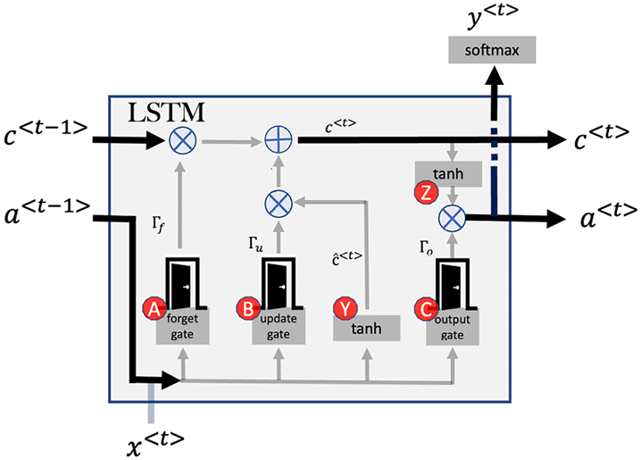
Figure 10.13: LSTM architecture
The candidate cell state
In LSTM, at each timestep, a candidate cell state, ![]() , is calculated, which is annotated as Y in Figure 10.13, and is the proposed new state for the memory cell. It is calculated using the current input
, is calculated, which is annotated as Y in Figure 10.13, and is the proposed new state for the memory cell. It is calculated using the current input ![]() and the previous hidden state
and the previous hidden state ![]() as follows:
as follows:
![]()
The update gate
The update gate is also called the input gate. The update gate in LSTM networks is a mechanism that allows the network to selectively incorporate new information into the current state so that the memory can focus on the most relevant information. It is annotated as B in Figure 10.13.
It is responsible for determining whether the candidate cell state ![]() should be added to
should be added to ![]() . It is implemented as a sigmoid layer that takes as input the current input
. It is implemented as a sigmoid layer that takes as input the current input ![]() and the previous hidden state:
and the previous hidden state:
![]()
The output of the sigmoid layer, ![]() , is a vector of values between 0 and 1, where each value corresponds to a single cell in the LSTM’s memory. A value of 0 indicates that the calculated
, is a vector of values between 0 and 1, where each value corresponds to a single cell in the LSTM’s memory. A value of 0 indicates that the calculated ![]() should be ignored, while a value of 1 indicates that
should be ignored, while a value of 1 indicates that ![]() is significant enough to be incorporated in
is significant enough to be incorporated in ![]() . Being a sigmoid function, it can have any value between 0 and 1, which indicates that some of the information from
. Being a sigmoid function, it can have any value between 0 and 1, which indicates that some of the information from ![]() should be incorporated in
should be incorporated in ![]() , but not all.
, but not all.
The update gate allows the LSTM to selectively incorporate new information into the current state and prevent the memory from becoming flooded with irrelevant data. By controlling the amount of new information that is added to the memory state, the update gate helps the LSTM to maintain a balance between preserving the previous state and incorporating new information.
Calculating memory state
As compared to GRU, the main difference in LSTM is that instead of having a single update gate (as we have in GRU), we have separate gates for the update and forget mechanisms for hidden state management. Each gate determines what is the right mix of various states to optimally calculate both the long-term memory ![]() current cell state and the current hidden state,
current cell state and the current hidden state, ![]() . The memory state is calculated by:
. The memory state is calculated by:
![]()
Eq. 10.12 consists of two terms annotated as 1 and 2. Being an output of a sigmoid function, ![]() and
and ![]() can either be 0 or 1. It means:
can either be 0 or 1. It means:
![]()
![]()
In other words, if the gate is open, update the value of ![]() . Otherwise, just retain the old state.
. Otherwise, just retain the old state.
Thus, the update gate in a GRU is a mechanism that allows the network to selectively discard information from the previous hidden state so that the hidden state can focus on the most relevant information. This is shown in Figure 10.13, which shows how the state travels from left to right.
The output gate
The output gate in an LSTM network is annotated as C in Figure 10.13. It is responsible for determining which information from the current memory state should be passed on as the output of the LSTM. It is implemented as a sigmoid layer that takes as input the current input and the previous hidden state. The output of the sigmoid layer is a vector of values between 0 and 1, where each value corresponds to a single cell in the LSTM’s memory.
As it is a sigmoid function, it means that ![]() can be either close to 0 or 1.
can be either close to 0 or 1.
If ![]() is 1, then it means that the value from the previous state
is 1, then it means that the value from the previous state ![]() should be used to calculate.
should be used to calculate. ![]() If
If ![]() is 0, then it means that the value from the previous state
is 0, then it means that the value from the previous state ![]() should be forgotten.
should be forgotten.
![]()
A value of 0 indicates that the corresponding cell should not contribute to the output, while a value of 1 indicates that the cell should fully contribute to the output. Values between 0 and 1 indicate that the cell should contribute some, but not all, of its value to the output.
In LSTMs, after processing the output gate, the current state is passed through a tanh function. This function adjusts the values such that they fall within a range between -1 and 1. Why is this scaling necessary? The tanh function ensures that the LSTM’s output remains normalized and prevents values from becoming too large, which can be problematic during training due to potential issues like exploding gradients.
After scaling, the result from the output gate is multiplied by this normalized state. This combined value represents the final output of the LSTM at that specific timestep.
To provide a simple analogy: imagine adjusting the volume of your music so it’s neither too loud nor too soft, but just right for your environment. The tanh function acts similarly, ensuring the output is optimized and suitable for further processing.
The output gate is important because it allows the LSTM to selectively pass on relevant information from the current memory state as the output. It also helps to prevent irrelevant information from being passed on as the output.
This output gate generates the variable ![]() which determines that the contribution of the cell state is output to the hidden state:
which determines that the contribution of the cell state is output to the hidden state:
![]()
In LSTM, ![]() is used as input to the gates, whereas
is used as input to the gates, whereas ![]() is the hidden state.
is the hidden state.
In summary, the output gate in LSTM networks is a mechanism that allows the network to selectively pass on relevant information from the current memory state as the output so that the LSTM can generate appropriate output based on the relevant information it has stored in its memory.
Putting everything together
Let’s delve into the workings of the LSTM across multiple timesteps, as depicted by A in Figure 10.14.
Just like GRUs, LSTMs create a conduit – often referred to as an “information highway” – which helps ferry context across successive timesteps. This is illustrated in Figure 10.14. What’s fascinating about LSTMs is their ability to use long-term memory to transport this context.
As we traverse from one timestep to the next, the LSTM learns what should be retained in its long-term memory, denoted as ![]() . At the start of every timestep,
. At the start of every timestep, ![]() interacts with the “forget gate,” allowing some pieces of information to be discarded. Subsequently, it encounters the “update gate,” where new data is infused. This allows
interacts with the “forget gate,” allowing some pieces of information to be discarded. Subsequently, it encounters the “update gate,” where new data is infused. This allows ![]() to transition between timesteps, continually gaining and shedding information as dictated by the two gates.
to transition between timesteps, continually gaining and shedding information as dictated by the two gates.
Now, here’s where it gets intricate. At the close of every timestep, a copy of the long-term memory, ![]() , undergoes transformation via the tanh function. This processed data is then sieved by the output gate, culminating in what we term short-term memory,
, undergoes transformation via the tanh function. This processed data is then sieved by the output gate, culminating in what we term short-term memory, ![]() . This short-term memory serves a dual purpose: it determines the output at that specific timestep and lays the foundation for the subsequent timestep, as portrayed in Figure 10.14:
. This short-term memory serves a dual purpose: it determines the output at that specific timestep and lays the foundation for the subsequent timestep, as portrayed in Figure 10.14:
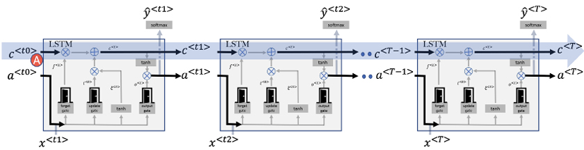
Figure 10.14: LSTM with multiple timesteps
Let us now look into how we can code RNNs.
Coding sequential models
For our exploration into LSTM, we’ll be diving into sentiment analysis using the well-known IMDb movie reviews dataset. Here, every review is tagged with a sentiment, positive or negative, encoded as binary values (True for positive, and False for negative). Our aim is to craft a binary classifier capable of predicting these sentiments based solely on the text content of the review.
In total, the dataset boasts 50,000 movie reviews. For our purposes, we’ll be dividing this equally: 25,000 reviews for training our model, and the remaining 25,000 for evaluating its performance.
For those seeking a deeper dive into the dataset, more information is available at Stanford’s IMDB Dataset.
Loading the dataset
First, we need to load the dataset. We will import this dataset through keras.datasets. The advantage of importing this dataset through keras.datasets is that it has been processed to be used for machine learning. For example, the reviews have been individually encoded as a list of word indexes. The overall frequency of a particular word has been chosen as the index. So, if the index of the word is “7,” it means that it is the 7th most frequent word. The use of pre-prepared data allows us to focus on the RNN algorithm instead of data preparation:
import tensorflow as tf
from tensorflow.keras.datasets import imdb
vocab_size = 50000
(X_train,Y_train),(X_test,Y_test) = tf.keras.datasets.imdb.load_data(num_words= vocab_size)
Note that the argument num_words=50000 is used to select only the top 50000 words. As the frequency of a word is used as the index, it means all the words with indexes less than 50000 are filtered out:
"I watched the movie in a cinema and I really like it"
[13, 296, 4, 20, 11, 6, 4435, 5, 13, 66, 447,12]
When working with sequences of varying lengths, it’s often beneficial to ensure that they all have a uniform length. This is particularly crucial when feeding them into neural networks, which often expect consistent input sizes. To achieve this, we use padding—adding zeros at the beginning or end of sequences until they reach a specified length.
Here’s how you can implement this with TensorFlow:
# Pad the sequences
max_review_length = 500
x_train = tf.keras.preprocessing.sequence.pad_sequences(x_train, maxlen=max_review_length)
x_test = tf.keras.preprocessing.sequence.pad_sequences(x_test, maxlen=max_review_length)
Indexes are great for the consumption of algorithms. For human readability, we can convert these indexes back to words:
word_index = tf.keras.datasets.imdb.get_word_index()
reverse_word_index = dict([(value, key) for (key, value) in word_index.items()])
def decode_review(padded_sequence):
    return " ".join([reverse_word_index.get(i - 3, "?") for i in padded_sequence])
Note that word indexes start from 3 instead of 0 or 1. The reason is that the first three indexes are reserved.
Next, let us look into how we can prepare the data.
Preparing the data
In our example, we are considering a vocabulary of 50,000 words. This means that each word in the input sequence ![]() will be encoded using a one-hot vector representation, where the dimension of each vector is 50,000. A one-hot vector is a binary vector that has 0s in all positions except for the index corresponding to the word, where it has a 1. Here’s we can load the IMDb dataset in TensorFlow, specifying the vocabulary size:
will be encoded using a one-hot vector representation, where the dimension of each vector is 50,000. A one-hot vector is a binary vector that has 0s in all positions except for the index corresponding to the word, where it has a 1. Here’s we can load the IMDb dataset in TensorFlow, specifying the vocabulary size:
vocab_size = 50000
(x_train, y_train), (x_test, y_test) = tf.keras.datasets.imdb.load_data(num_words=vocab_size)
Note that as vocab_size is set to 50,000, so the data will be loaded with the 50,000 most frequently occurring words. The remaining words will be discarded or replaced with a special token (often denoted as <UNK> for “unknown”). This ensures that our input data is manageable and only includes the most relevant information for our model. The variables x_train and x_test will contain the training and testing input data, respectively, while y_train and y_test will contain the corresponding labels.
Creating the model
We begin by defining an empty stack. We’ll use this for building our network, layer by layer:
model = tf.keras.models.Sequential()
Next, we’ll add an Embedding layer to our model. If you recall our discussion about word embeddings in Chapter 9, we used them to represent words in a continuous vector space. The Embedding layer serves a similar purpose but within the neural network. It provides a way to map each word in our vocabulary to a continuous vector. Words that are close to one another in this vector space are likely to share context or meaning.
Let us define the Embedding layer, considering the vocabulary size we chose earlier and mapping each word to a 50-dimensional vector, corresponding to the dimension of ![]() :
:
model.add(
    tf.keras.layers.Embedding(
        input_dim = vocab_size,
        output_dim = 50,
        input_length = review_length
    )
)
Dropout layers prevents overfitting and force the model to learn multiple representations of the same data by randomly disabling neurons in the learning phase. Let us randomly disable 25% of the neurons to deal with overfitting:
model.add(
    tf.keras.layers.Dropout(
        rate=0.25
    )
)
Next, we’ll add an LSTM layer, which is a specialized form of RNN. While basic RNNs have issues in learning long-term dependencies, LSTMs are designed to remember such dependencies, making them suitable for our task. This LSTM layer will analyze the sequence of words in the review along with their embeddings, using this information to determine the sentiment of a given review. We’ll use 32 units in this layer:
model.add(
    tf.keras.layers.LSTM(
        units=32
    )
)
Add a second Dropout layer to drop 25% of neurons to reduce overfitting:
model.add(
    tf.keras.layers.Dropout(
        rate=0.25
    )
)
All LSTM units are connected to a single node in the Dense layer. A sigmoid activation function determines the output from this node – a value between 0 and 1. Closer to 0 indicates a negative review. Closer to 1 indicates a positive review:
model.add(
    tf.keras.layers.Dense(
        units=1,
        activation='sigmoid'
    )
)
Now, let us compile the model. We will use binary_crossentropy as the loss function and Adam as the optimizer:
model.compile(
    loss=tf.keras.losses.binary_crossentropy,
    optimizer=tf.keras.optimizers.Adam(),
    metrics=['accuracy'])
Display a summary of the model’s structure:
model.summary()
__________________________________________________________________________
Layer (type)               Output Shape               Param #
=========================================================================
embedding (Embedding)      (None, 500, 32)            320000
dropout (Dropout)          (None, 500, 32)            0
lstm (LSTM)                (None, 32)                 8320
dropout_1 (Dropout)        (None, 32)                 0
dense (Dense)              (None, 1)                  33
=========================================================================
Total params: 328,353
Trainable params: 328,353
Non—trainable params: 0
Training the model
We’ll now train the LSTM model on our training data. Training the model involves several key components, each of which is described below:
- Training Data: These are the features (reviews) and labels (positive or negative sentiments) that our model will learn from.
- Batch Size: This determines the number of samples that will be used in each update of the model parameters. A higher batch size might require more memory.
- Epochs: An epoch is a complete iteration over the entire training data. The more epochs, the more times the learning algorithm will work through the entire training dataset.
- Validation Split: This fraction of the training data will be set aside for validation and not be used for training. It helps us evaluate how well the model is performing.
- Verbose: This parameter controls how much output the model will produce during training. A value of 1 means that progress bars will be displayed:
history = model.fit(
    x_train, y_train,    # Training data
    batch_size=256,
    epochs=3,
    validation_split=0.2,
    verbose=1
)
Epoch 1/3 79/79 [==============================] - 75s 924ms/step - loss: 0.5757 - accuracy: 0.7060 - val_loss: 0.4365 - val_accuracy: 0.8222 Epoch 2/3 79/79 [==============================] - 79s 1s/step - loss: 0.2958 - accuracy: 0.8900 - val_loss: 0.3040 - val_accuracy: 0.8812 Epoch 3/3 79/79 [==============================] - 73s 928ms/step - loss: 0.1739 - accuracy: 0.9437 - val_loss: 0.2768 - val_accuracy: 0.8884
Viewing some incorrect predictions
Let’s have a look at some of the incorrectly classified reviews:
predicted_probs = model.predict(x_test)
predicted_classes_reshaped = (predicted_probs > 0.5).astype("int32").reshape(-1)
incorrect = np.nonzero(predicted_classes_reshaped != y_test)[0]
We select the first 20 incorrectly classified reviews:
class_names = ["Negative", "Positive"]
for j, incorrect_index in enumerate(incorrect[0:20]):
    predicted = class_names[predicted_classes_reshaped[incorrect_index]]
    actual = class_names[y_test[incorrect_index]]
    human_readable_review = decode_review(x_test[incorrect_index])
    print(f"Incorrectly classified Test Review [{j+1}]")
    print(f"Test Review #{incorrect_index}: Predicted [{predicted}] Actual [{actual}]")
    print(f"Test Review Text: {human_readable_review.replace('<PAD> ', '')}
")
Summary
The foundational concepts of sequential models were explained in this chapter, which aimed to give you a basic understanding of the techniques and methodologies of such techniques. In this chapter, we presented RNNs, which are great for handling sequential data. A GRU is a type of RNN that was introduced by Cho et al. in 2014 as a simpler alternative to LSTM networks.
Like LSTMs, GRUs are designed to learn long-term dependencies in sequential data, but they do so using a different approach. GRUs use a single gating mechanism to control the flow of information into and out of the hidden state, rather than the three gates used by LSTMs. This makes them easier to train and requires fewer parameters, making them more efficient to use.
The next chapter introduces some advanced techniques related to sequential models.
Learn more on Discord
To join the Discord community for this book – where you can share feedback, ask questions to the author, and learn about new releases – follow the QR code below: