8.2. Framing the Problem

To frame the problem, Carl and his team develop a formal project charter. Additionally, they obtain customer input that directs them to focus on two critical process characteristics, melt flow index and color index.

8.2.1. Developing a Project Charter

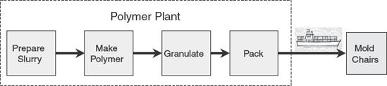
During their first team meeting, Carl and his team members draw a high-level process map (Exhibit 8.3). They also decide to review yield data from both the polymer and molding plants to confirm the size and frequency of the problem.

Figure 8.3. High-level Process Map of White Polymer Molding Process

There have been many arguments about white polymer quality. Although there is a polymer specification, the molding plant has long suspected that it does not fully reflect the true requirements of their process. After a long discussion, the team agrees on the following Key Performance Indicator (KPI) definition for the project:

Daily yield, calculated as the weight of good polymer divided by the weight of total polymer produced.

Good polymer is polymer that can be successfully processed by the molding plant.

Total polymer produced will include product that fails to meet the polymer plant specifications, plus any polymer that, although meeting polymer plant specifications, is subsequently scrapped or rejected in the molding plant.

Carl collects some historical data on daily yield and imports it into a data table that he names BaselineYieldData.jmp. Part of this data table is shown in Exhibit 8.4. The data table contains two columns, Date and Yield, and covers a period of a little over three years.

Figure 8.4. Partial View of BaselineYieldData.jmp

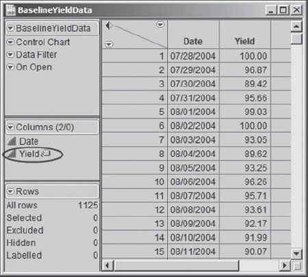
Note that Carl has designated Yield as a Label variable, as evidenced by the yellow label icon next to Yield in the columns panel in Exhibit 8.4. He did this by right-clicking on Yield in the columns panel and selecting Label/Unlabel. With this property, when the arrow tool hovers over a point in a plot, that point's value of Yield will appear. Carl thinks this may be useful later on.

Carl decides to construct an individual measurement (IR) control chart to see how Yield varies over time. He realizes that the distribution of Yield measurements is likely to be skewed since there is an upper limit of 100 percent, so control limits calculated using an individual measurement control chart may not be appropriate. Nonetheless, he decides to use the individual measurement chart in an exploratory fashion.

To construct this chart, he selects Graph > Control Chart > IR. In the dialog he enters Yield as Process and Date as Sample Label. As shown in Exhibit 8.5, he also unchecks the Moving Range (Average) box, as this is not of interest to him at this point—he is only interested in the IR chart. Carl then clicks OK.

Figure 8.5. Launch Dialog for IR Chart of Baseline Yield Data

The resulting chart is shown in Exhibit 8.6. This chart clearly shows periods of high yields, each followed by a crisis, with a total of nine crises over the period (two of these crisis periods are marked in Exhibit 8.6). The average Yield over this time period is about 88 percent, and Carl notes that, as expected, the process is far from stable.

Figure 8.6. IR Chart of Baseline Yield Data

Following good documentation practice, Carl saves a script to the data table to reproduce this chart. He does this by clicking on the red triangle next to Control Chart in the report window and choosing Script > Save Script to Data Table. By default, the script is called Control Chart.

Recall that Carl has designated Yield as a Label variable. To get some idea of what the noncrisis Yield values might be, Carl lets his arrow tool hover over various points to see their yields, and decides that crisis periods can be loosely defined by collections of batches with Yield values below 85.

Carl is curious about the likely yield of the process had it not been affected by these crisis periods. Just to get a sense of the noncrisis yields, he decides to construct a control chart with crisis batches, defined as batches with yields below 85, excluded. The Data Filter, found under Rows, provides an easy way to filter out data values. Carl selects Rows > Data Filter. In the dialog window that appears, he selects Yield and clicks Add. The dialog window now appears as in Exhibit 8.7.

Figure 8.7. Data Filter Dialog with Yield Added

Carl would like to include only those rows with yields of at least 85. To do this, Carl clicks on the minimum value for Yield above the slider in the dialog box; this is shown as 41.905 in Exhibit 8.7. When he clicks on 41.905, a text box appears into which he types 85. Because Select is checked, the Data Filter selects all rows where Yield is at least 85. To include only these rows in calculations, Carl checks the Include box. But he also unchecks Select, because he does not need to have these rows selected.

Now Carl's dialog appears as shown in Exhibit 8.8. He checks his data table to see that 280 rows have been excluded and scrolls to verify that these are the crisis yield rows. He clicks on the red arrow in the report window next to Data Filter and selects Script > Save Script to Data Table. This saves the script for the data filter with the default name Data Filter.

Figure 8.8. Data Filter Dialog Settings to Exclude Crisis Rows

Now that crisis rows have been excluded, Carl reruns his Control Chart script. His new control chart is shown in Exhibit 8.9. Although the crisis points were excluded from the control chart calculations, they were not hidden, so they appear gray on the plot. This is good—Carl did not want anyone to forget that these periods had occurred. He notes that the overall Yield for the noncrisis days is about 94 percent. This will help him and his teammates determine a goal for their project.

Figure 8.9. IR Chart with Crisis Periods Excluded

Carl closes his data table at this point. With this information as background, the team reconvenes to agree upon the problem statement and project goal, and to define the specific scope and focus of the project.

The team drafts a project charter, shown in Exhibit 8.10. As instructed, the team members decide to focus on the polymer plant. They set a goal of achieving an average yield of 95 percent by the end of the year. It is late August—this gives them four months. They know that if they can eliminate the crises, they can expect a 94 percent yield. But, knowing that they will be constructing detailed knowledge of the process, they feel that they can even do a little better.

Figure 8.10. Project Charter

At this point, Carl checks in with Edward to ensure that he is comfortable with the project charter and the team's proposed direction. Edward is very impressed with the clarity of the team's work to date and likes the idea that the project goal was chosen based on sound data. He is quick to approve of the team's charter and direction.

8.2.2. Identifying Customer Requirements

Next, the team members need to explore the following questions:

• What are the true requirements of the molding plant?

• Why are these requirements met at some times but not at others?

• What is changing?

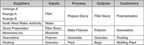
To this end, during their next meeting, they produce a SIPOC map to help them gain a better understanding of the process steps and to identify where they should focus within the polymer plant (Exhibit 8.11).

Figure 8.11. SIPOC Map for White Polymer Process

The team also proceeds to collect voice of the customer (VOC) information from the immediate customers of the process, namely, the stakeholders at the molding plant. Through interviews, team members collect information from molding plant technicians and managers. There are many comments reflecting that plant's frustration, such as the following:

• "I don't want any crises caused by poor polymer."

• "Your polymer is not consistent."

• "I don't believe you when you say you are in spec."

• "I need to be able to make good white molding all the time."

• "You are killing my business."

• "We can't continue with these scrap levels."

But the team also collects specific information about the technical requirements of the molding process. They diagram their analysis in the form of a Critical to Quality tree, a portion of which is shown in Exhibit 8.12. Two primary characteristics quickly emerge:

• The molding plant has specified that in order for the polymer to process well on their equipment, the polymer's melt flow index, or MFI, must fall between lower and upper specification limits of 192 and 198 (with a target of 195).

• The polymer's color index, or CI, must meet the whiteness specification. The maximum possible CI value is 100, but the only requirement is that CI must exceed a lower specification limit of 80.

  Figure 8.12. Partial Critical to Quality Tree for Molding Plant VOC