5.1.1 Normalization

Normalization is used to reduce the variations in gray level values along ridges and valleys by adjusting the range of gray level values [16, 28]. In normalization, an input fingerprint image is normalized so that the image has a prespecified mean and variance. Let I(x, y) and N (x, y) denote the intensity value of input fingerprint image and normalized image at pixel (x, y). The normalization is done using Eq. (5.1) [16].

Figure 5.2: Preprocessing of fingerprint image.

(5.1)

In Eq. (5.1), M and V are the estimated mean and variance of I(x, y), respectively, and M₀ and V₀ are the desired mean and variance values, respectively.

5.1.2 Segmentation

In this step, the foreground fingerprint region which contains the ridges and valleys is separated from the image. The foreground region has a very high gray scale variance value [28]. Hence, a variance based thresholding method [16] is used for segmentation. First, the normalized fingerprint image is divided into a number of non-overlapping blocks and the gray scale variance is calculated for each block. Next, the foreground blocks and background blocks are decided based on a global threshold value. The threshold value is fixed for all blocks. Then, the gray-scale variance value of each block is compared with the global threshold value. If the variance is less than the global threshold value, then the block is assigned as background region, otherwise, it is assigned as foreground region. Finally, the background region is removed from the image and the fingerprint region is identified which is used in subsequent stages of preprocessing and feature extraction.

5.1.3 Local Orientation Estimation

The orientation field of a fingerprint image represents the local orientation of the ridges and valleys in a local neighborhood. To compute the orientation image, Hong et al. [16] least mean square estimation method is used. In this method, block-wise orientations of the segmented image are calculated. First, the whole image is divided into a number of blocks each of size 16 × 16 and the gradient ∂_x and ∂_y along x- and y- axis are calculated, respectively. The gradients are computed using Sobel operator [14]. Next, the local orientation θ of each block centered at pixel (x, y) is calculated using Eq. (5.2), (5.3) and (5.4) [16].

(5.2)

(5.3)

(5.4)

Finally, smoothing of the orientation field in a local neighborhood is performed to remove the noise present in the orientation image. For this purpose, the orientation image is converted into a continuous vector field and then Gaussian filter [16, 28] is applied on the orientation image for smoothing.

5.1.4 Local Frequency Image Representation

The frequency image represents the local ridge frequency which is defined as the frequency of the ridge and valley structures in a local neighborhood along a direction normal to the local ridge orientation [16]. Local ridge frequency can be computed as the reciprocal of the number of pixels between two consecutive ridges in a region. Hong et al. [16] method is used to calculate the ridge frequency. In this method, the normalized fingerprint image is divided into a number of non-overlapping blocks. An oriented window is defined in the ridge coordinate system along a direction orthogonal to the local ridge orientation at the center pixel for each block. The average number of pixels between two consecutive ridges are calculated. Let T(x, y) be the average number of pixels of block centered at (x, y). Then, the frequency F (x, y) of the block (x, y) is calculated using Eq. (5.5) [16].

(5.5)

If no consecutive peaks are there in the block, then the frequency of the block is assigned a value of −1 to differentiate it from the valid frequency values.

5.1.5 Ridge Filtering

A 2-D Gabor filter is used to remove efficiently the undesired noise and enhance the ridge and valley structures of the fingerprint image. The Gabor filter is employed because it has both frequency and orientation selective properties [28] which adjust the filter to give maximal response to ridges at a specific orientation and frequency in the fingerprint image. Therefore, the Gabor filter preserves the ridge and valley structures and also reduces noise. An even-symmetric Gabor filter tuned with local ridge frequency and orientation is used to filter the ridges in a fingerprint image. The orientation and frequency parameters of the even-symmetric Gabor filter are determined by the ridge orientation and frequency information of the fingerprint. The detailed method can be found in [16].

5.1.6 Binarization and Thinning

The binarization is used to improve the contrast between the ridges and valleys in a fingerprint image by converting a gray level image into a binary image [28]. The binary image is useful for the extraction of minutiae points. The gray level value of each pixel is checked in the enhanced image. If the value is greater than a predefined threshold value, then the pixel value is set to one, otherwise, it is set to zero. The binary image contains two levels of information, the foreground ridges and the background valleys.

Finally, thinning morphological operation is performed prior to the minutiae extraction. Thinning is performed by successively eroding the foreground pixels until they are one pixel wide. A standard thinning algorithm [15] is used to perform thinning operation. This algorithm performs thinning using two sub iterations. In each subiteration, the neighborhood of each pixel is examined in the binary image based on a particular set of pixel-detection criteria, whether the pixel can be deleted or not. These processes continue until there are no more pixels for deletion. It may be noted that the application of the thinning algorithm to a fingerprint image preserves the connectivity of the ridge structures while forming a thinning image of the binary image. This thinned image is then used in the subsequent minutiae extraction process.

5.1.7 Minutiae Point Extraction

Two main minutiae features namely ridge ending and ridge bifurcation are considered in this work. The Crossing Number (CN) [25, 28] method is followed to extract these minutiae features. This method extracts the ridge endings and bifurcations from the thinned image by scanning the local neighborhood of each ridge pixel using a 3 × 3 window [25]. A 3 × 3 window centered at point P and its eight neighbor points P_i (i = 1, 2, ... , 8) are shown in Fig. 5.3(a). The CN at point P is defined as half the sum of the differences between pairs of adjacent pixels in the eight-neighborhood (see Eq. (5.6)) [25, 28]. Note that value of each P_i (i = 1, 2, . . . , 8) is either 0 or 1, as the image is binarized (see Section 5.1.6).

Figure 5.3: Pixel position and crossing number for two different types of minutiae.

(5.6)

Using the properties of the CN, the ridge ending and bifurcation are detected for CN = 1 and CN = 3, respectively. Figure 5.3(b) shows a ridge ending with C N = 1 and Fig. 5.3(c) shows a bifurcation minutiae point with C N = 3.

ANSI/NIST-ITL format [24] is used to store the minutiae points. The origin of the fingerprint image is located at the bottom-left corner and y-coordinate is measured from the bottom to upward. The position and the angle of a minutiae feature are stored in (x, y, θ, T) format where (x, y) is the location coordinate of a minutiae in the fingerprint image, θ is the minutiae angle and T is the type of minutiae. The value of T is R for ridge end type minutiae and B for bifurcation type minutiae. Minutiae angle (θ) is measured anti-clockwise with the horizontal x-axis. The angle of a ridge ending is calculated by measuring the angle between the horizontal x-axis and the line starting at the ridge end point and running through the middle of the ridge as shown in Fig. 5.4(a). The angle of a bifurcation is calculated by measuring the angle between the horizontal x-axis and the line starting at the minutia point and running through the middle of the intervening valley between the bifurcating ridges as shown in Fig. 5.4(b).

Extracted minutiae using the above mentioned method may have many false minutiae due to breaks in the ridge or valley structures. These artifacts are typically introduced by the noise at the time of taking fingerprint impression. A break in a ridge causes two false ridge endings to be detected, while a break in a valley causes two false bifurcations. In order to remove all these false minutiae, the shorter distance minutiae removal method of Chatterjee et al. [13] is followed. In this method, the distance between two ridge ending points or two bifurcation points, and orientations of that points are checked. If the distance is less than some minimum distance say δ, and the orientations of two points are opposite, then both minutiae points are removed. Here, the distance between two points is considered as Euclidean distance. Euclidean distance (ED) between two minutiae points A and B with positions (x_A, y_A) and (x_B, y_B) is defined as:

(5.7)

Figure 5.4: Minutiae position and minutiae orientation.

Let two minutiae points A and B are represented as (x_A, y_A, θ_A, T_A) and (x_B,y_B,θ_B,T_B), respectively. The Euclidean distance between two minutiae points is represented as ED(A, B). The following heuristic is applied to remove the false minutiae points.

In the above heuristic, the value of δ is chosen as the average distance between two ridges in the fingerprint image whose value is typically taken as 10. The difference of the orientations (|θ_A − θ_B |) is checked between 150 to 210 degree for the oppositeness of the minutiae points. Note that the exact value of |θ_A − θ_B| is 180 degree when the minutiae points are opposite. The tolerance value of ±30 degree is considered due to the curvature nature of the ridges.

5.2.1 Two Closest Points Triangulation

To capture the structural information from the distribution of minutiae points, the concept of two closest point triangulation is proposed. A two closest point triangle is defined with three minutiae points such that for any point, the distance from other two points are minimum. In other words, let m_i be a minutiae point. Other two points say m_j and m_k form a two closest point triangle if the distances between m_i and m_j , and m_i and m_k are minimum compared to all other minutiae points in the fingerprint. Figure 5.5(a) illustrates the definition of the two closest point triangle with four minutiae points. It may be noted that the triangulation covers less geometric area of a fingerprint and implies a meaningful feature. A set of two closest point triangles can be obtained from a given fingerprint image. Figure 5.5(b) shows the two closest point triangles obtained from minutiae points of a sample fingerprint.

5.2.2 Triplet Generation

A two closest point triangle with three minutiae points represents a triplet. First, all such triplets are identified. Let M = {m₁, m₂, ... , m_{|M |}} be a set of |M | minutiae points in a fingerprint image. A set of minutiae triplets T = {t₁, t₂,...,t_{|T |}} from M need to be identified. The number of triplets in the set T is |T|, where |T| = |M|. First, the distance matrix D is calculated as shown in Eq. (5.8). Each entry in D denotes the distance between two minutiae points. For example, d_i,j represents the distance between the i^th and j^th minutiae points. Here, d_i,j is calculated as the Euclidean distance using Eq. (5.7).

(5.8)

The triplet corresponding to the i^th minutiae m_i in the triplet set T is represented with t_i, where t_i =< m_i, m_j , m_k > and 1 ≤ i, j, k ≤ |M|. The minutiae points m_j and m_k of triplet t_i are determined by the criteria defined in Eq. (5.9).

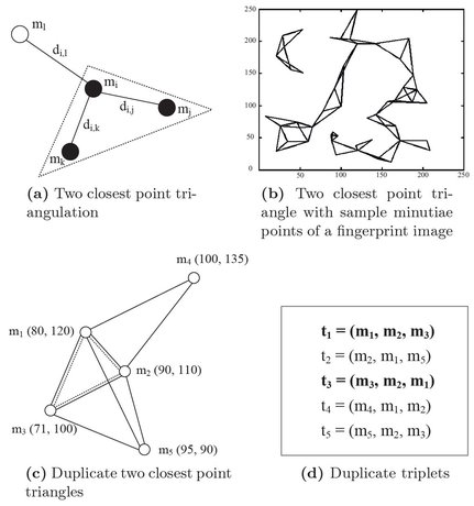
Figure 5.5: Two closest point triangulation with sample fingerprint.

(5.9)

In Eq. (5.9), minIndex function returns the minutiae point having the minimum distance from the i^th minutiae. Each t_i generated using the above mentioned criteria is added to the triplet set T. Note that there may be duplicate triplets in T because the minutiae points with the minimum distance may be same for two neighborhood points. Figure 5.5(c) and (d) show the closest point triangles and corresponding triplets generated from the five minutiae points of Fig. 5.5(c). Initially, the number of triplets in T is 5. It can be shown that the triplets t₁ and t₃ generated from minutiae points m₁ and m₃ are same. Hence, one of these duplicate triplets (t₁ or t₃) is removed from T. After removing the triplet t₃, the set contains t₁, t₂, t₄ and t₅.

In this way, the triplet set T is generated, where |T| is the number of triplets generated from |M | minutiae points. It may be noted that |T | is at most equal to |M | for a fingerprint image.

5.4.1 Linear Index Space

In this approach, all index keys and subject identities are stored linearly. In other words, a 2-D index space is created to store index keys and the corresponding identities. The size of the index space would be N × (F L + 1) where N is the total number of index keys generated from all persons and F L (F L = 8) is the number of feature values in an index key. The first eight columns of each row in the 2-D space contain the eight feature values of an index key and the last column contains the identity of the subject corresponding to the index key. The method of creating linear index space is summarized in Algorithm 5.1. In Step 2 to 12 of Algorithm 5.1, all index keys and identity of a person are stored in the linear index space. Among these steps, Step 5 to 7 store the eight key values into the first eight columns of the linear index space and Step 8 stores the identity of the person into the 9^th column of the linear index space.

Figure 5.7 shows the structure of the linear index space in the database. In Fig. 5.7, LNINDX is the two dimensional index space of size N × (FL + 1). In this structure, number of index keys can be stored from the P subjects with Q samples each. Here, first all index keys of the 1^st subject are stored, then all index keys of the 2^nd subject and so on. In Fig. 5.7, the entry > and in LNINDX represent the i^th index key and the identity of the q^th sample of the p^th subject, respectively.

Algorithm 5.1 Creating linear index space

5.4.2 Clustered Index Space

In this approach, all index keys are divided into a number of groups. The grouping is done by performing k-means clustering on all index keys using the 8-dimensional feature values. number of clusters are chosen which is the rule of thumb of clusters for any unsupervised clustering algorithm [23] to balance between the number of clusters and the number of items within a single cluster. An eight dimensional index key is treated as a eight dimensional point in the cluster space. Before doing k-means clustering, the fingerprint data is preprocessed so that clustering algorithm converges to a local optima. In preprocessing, the distances of all points from the origin are compared and the density of the points from the distance histogram is found. From this histogram, the top picks are selected and the cluster centers are randomly initialized with these points. Then, the k-means clustering is applied on all eight dimensional points in the cluster space (i.e. all index keys) and the centroid is found for each cluster. The cluster centroid represents the point which is equal to the average values of all the eight dimensional points in the cluster. Then, key points are assigned to the clusters such that the distance of a key point from the centroid of assigned cluster is the minimum than the distances from the centroids of other clusters. If any key point is found with almost same distances from the two or more cluster centers and or some isolated points with large distance from cluster center, those points are removed from the resulting partition to reduce the effect of outliers.

Figure 5.7: Linear index space.

The distance is measured as Euclidean distance between key point and cluster centroid. Finally, when all points are assigned, the centroids of the cluster is recalculated. The centroid of each cluster is stored in a two dimensional space (see Fig. 5.8). The size of the space is K × (F L + 1), where K is the number of clusters (here, and F L (F L = 8) is the number of features in an index key.

Let N_i be the number of index keys present in the i^th cluster and ƒ^j(l) be the l^th (l = 1, 2, . . . , 8) feature value of the j^th index key in the i^th cluster. Then, the l^th centroid value dcnⁱ(l) of the i^th cluster is calculated using Eq. (5.18).

(5.18)

Thus, eight centroid index values (dcnⁱ(1) dcnⁱ(2) · · · dcnⁱ(8)) can be calculated of the i^th cluster using Eq. (5.18) and the centroid values are stored in a 2-D space (CLTCNTRD in Fig. 5.8). In Fig. 5.8, CLTCNTRD is the array for storing the centroid values of all clusters. The first eight columns of each row store the 8-dimensional centroid values (dcn(l), l = 1, 2, . . . , 8) for a cluster and the last column stores the cluster id (it is represented as clid in Fig. 5.8) which uniquely identifies each cluster. For each cluster, a linear index space (Cluster → LNINDX) is created as shown in Fig. 5.8. In Fig. 5.8, Cluster[i] → LNINDX is the linear index space for the i^th cluster. The feature values of an index key in Cluster[i] → LNINDX are denoted as < f(1),f(2),··· ,f(8) > and the identity of the subject corresponding to the index key is represented as id. Note that the index keys within a cluster are stored in a linear fashion. The method for creating clustered index space is summarized in Algorithm 5.2. In Step 2 to 12 of Algorithm 5.2, all index keys of all samples of all subjects are stored into a linear index space. In Step 13, k-meansClustering function takes the linear index space as input and divides all index key into K groups. Each group is stored in Cluster[ ] → LNINDX [ ] [ ] 2-D space of the clustered index space. In Step 15, Centroid function calculates the centroid of a cluster. The centroid values of a cluster are stored in CLTCNTRD of cluster index space. The cluster id of each cluster (here cluster number) is stored in the 9^th column of CLTCNTRD in Step 16.

Figure 5.8: Clustered index space.

5.4.3 Clustered kd-tree Index Space

First, clusters of all index keys are created as discussed above. Then each index key of a cluster is stored into a kd-tree. A kd-tree is a data structure for storing a finite set of points from a k-dimensional space [7]. The kd-tree is a binary tree in which every node stores a k-dimensional point. In other words, the node of a kd-tree stores an eight dimensional point. The node structure of kd-tree is shown in Fig. 5.9(a). In a node of a kd-tree, keyV ector field stores the k-dimensional index key and Split field stores the splitting dimension or a discriminator value. The leftTree and rightTree store a kd-tree representing the pointers to the left and right of the splitting plane, respectively. For an example, let there are twelve three dimensional points (P1, P2, . . . , P12) as shown in Fig. 5.9(b) and a kd-tree with these points is shown in Fig. 5.9(c). The first point P1 is inserted at the root of the kd-tree. At the time of insertion, one of the dimension is chosen as a basis (Split) of dividing the rest of the points. In this example, the value of Split in the root node is 1. In other words, if the value of the first dimension of the current point to be inserted is less than the same of the root, then the point is stored in leftTree otherwise in rightTree. This means all items to the left of root will have the first dimension value less than that of the root and all items to the right of the root will have greater than (or equal to) that of the root. The point P2 is inserted in the right kd-tree and P3 is inserted in the left kd-tree of the root. When the point P4 is inserted, the first dimension value of P4 is compared with the root and then the second dimension value of P4 is compared with the second dimension value of P2 at next level. The point P4 is inserted in the right kd-tree of the point P2. Similarly, all other points are inserted into the kd-tree. First dimension will be chosen again as the basis (Split=1 ) for discrimination at level 3. All eight dimensional points (index keys) are stored within a cluster in a kd-tree data structure. The FLANN library [1, 5, 26] is used to implement the kd-tree in this work. The maximum height of the optimized kd-tree with N number of k-dimensional point is [log₂(N)] [7].

Algorithm 5.2 Creating clustered index space

Figure 5.9: Structure of a kd-tree and an example of kd-tree with three dimensional points.

Figure 5.10 shows the schematic of a clustered kd-tree index space. In Fig. 5.10, CLTCNTRD stores the centroid of the K clusters. The centroid value of the i^th cluster is represented as < dcnⁱ(l) dcnⁱ(2) · · · dcnⁱ(8) >. The index keys within a cluster are stored into a kd-tree data structure and a unique id is assigned to the each kd-tree. The id of a kd-tree is stored at the last column of the CLTCNTRD. In Fig. 5.10, rootⁱ represents the id of the i^th kd-tree. The kd-treeⁱ stores the index keys of the i^th cluster as shown in Fig. 5.10.

The methods for creating clustered kd-tree index spaces are summarized in Algorithm 5.3. In Step 2 to 12 of Algorithm 5.3, all index keys of all samples of all subjects are stored in a linear index space.

Figure 5.10: Clustered kd-tree index space.

Algorithm 5.3 Creating clustered kd-tree index space

Step 13 takes the linear index space as input and divides all index keys into k groups using k-meansClustering function. In Steps 14 to 20 of Algorithm 5.3, the clustered kd-tree index space is created. In Step 15, Centroid function calculates the centroid of a cluster. The centroid values of a cluster are stored in CLTCNTRD of clustered index space. In Step 16 to 18, each index key of the k^th cluster is inserted into the k^th kd-tree and in Step 19, the id of the k^th kd-tree is stored in the 9^th column of k^th row of clustered index space (CLTCNTRD).

5.5.1 Linear Search (LS)

In this approach, the linear index space is searched for a query fingerprint. For an index key of the query fingerprint, whole linear index space is searched and the distances are calculated with all index key stored in linear index space. The distance is calculated as Euclidean distance. The Euclidean distance between the i^th index key of the query fingerprint and the j^th index key of the q^th sample of the p^th subject in the database is calculated as in Eq. (5.20).

(5.20)

The identity is stored and a vote is casted on that identity in the CSET corresponding to the minimum distance. If the j^th index key in the database produces minimum Euclidean distance for the i^th index key of query fingerprint, then a vote is added for the subject identity (Id^j ) of the j^th index key. In the similar way, the votes are casted for other index keys of the query fingerprint. The identity which receives the highest number of votes will be ranked first in the CSET. The method for generating CSET using linear search is described in Algorithm 5.4. Step 3 to 7 of Algorithm 5.4 calculate the distances between a query index key and all stored index keys. In Step 8, the minimum distance among all calculated distances is determined. Match index corresponding to the minimum distance is selected in Step 9 and the id is retrieved from linear index space at that index in Step 10. Step 11 to 18 generate the CSET and CSET is sorted according to received votes in Step 20.

5.5.2 Clustered Search (CS)

In this technique, the clustered index space is searched to retrieve the candidate set. For an index key of query fingerprint, first a cluster is found which contains index keys similar with the query index key. Then, the all identities are retrieved from the identified cluster. To do this, first the Euclidean distance is calculated between an index key of the query fingerprint and all stored centroid values of clusters using Eq. (5.21). In Eq. (5.21), is the i^th index key of the query fingerprint and dcn^j is the centroid values of the j^th cluster.

(5.21)

The cluster is selected which has the minimum distance between a query index key and the centroid values of that cluster. If centroid values of the j^th cluster in the database produce minimum distance, then all identities are retrieved from the linear index space (Cluster[i] → LNINDX[ ][ ]) of the j^th cluster in the database. Similarly, the clusters are found for all other index keys of the query fingerprint. The voting is done with the retrieved identities from the clusters to generate the CSET. The method for generating CSET from the clustered index space is summarized in Algorithm 5.5. Step 2 to 7 of Algorithm 5.5 find the matched cluster for an index key of query fingerprint.

Algorithm 5.4 Candidate set generation in LS from linear index space

Algorithm 5.5 Candidate set generation in CS from clustered index space

5.5.3 Clustered kd-tree Search (CKS)

In this approach, first the cluster is found to which a query index key belongs. Then, the kd-tree is searched corresponding to that cluster. The cluster is found which have the minimum Euclidean distance between a query index key and the stored centroid index key. The method is discussed in the previous section. If centroid values of the i^th cluster produces minimum Euclidean distance, the i^th kd-tree is searched in the database. The method for creating CSET from the clustered kd-tree index space is summarized in Algorithm 5.6. Step 2 to 7 of Algorithm 5.6 find the matched cluster for an index key of the query fingerprint. Step 8 finds the nearest neighbors of query index key from the kd-tree corresponding to matched cluster. FLANN library [1, 5, 26] is used to search the kd-tree. The subject identity of the nearest neighbor is found in Step 9 and 10. The sorted CSET is generated in Step 11 to 19.

5.6.1 Databases

In this experiments, six widely used fingerprint databases are considered. The first two databases are obtained from National Institute of Science and Technology (NIST) Special DB4 database [4, 29]. The remaining databases are obtained from Fingerprint Verification Competition (FVC) 2004 databases [2, 22]. Detailed description of each database is given in the following.

Algorithm 5.6 Candidate set generation in CKS from clustered kd-tree index space

NIST DB4: The NIST Special Database 4 [4, 29] contains 4000 8-bit gray scale fingerprint images from 2000 fingers. Each finger has two different image instances (F and S). The fingerprint images are captured at 500 dpi resolution from rolled fingerprint impressions scanned from cards. The size of each fingerprint image is 512 × 512 pixels with 32 rows of white space at the bottom of the fingerprint image. The fingerprints are uniformly distributed in the five fingerprint classes: arch (A), left loop (L), right loop (R), tented arch (T) and whorl (W).

NIST DB4 (Natural): The natural distribution of fingerprint images [4, 18] is A = 3.7%, L = 33.8%, R = 31.7%, T = 2.9% and W = 27.9%. A subset of NIST DB4 is obtained by reducing the cardinality of the less frequent classes to resemble a natural distribution. The data set contains 1,204 fingerprint pairs (the first fingerprints from each class have been chosen according to the correct proportion).

FVC2004 DB1: The first FVC 2004 database [2, 22] contains 880 fingerprint images of 110 different fingers. Each finger has 8 impressions in the database. The images are captured at 500 dpi resolutions using optical sensor (“V300” by CrossMatch) [22]. The size of each image is 640 × 480 pixels.

FVC2004 DB2: The second FVC 2004 database [2, 22] contains 880 fingerprint images captured from 110 different fingers and 8 impressions per finger. The images are captured at 500 dpi resolutions using optical sensor (“U.are.U 4000” by Digital Persona) [22]. The size of each image is 328×364 pixels.

FVC2004 DB3: The third FVC 2004 database [2, 22] contains 880 fingerprint images of 110 different fingers captured at 512 dpi resolutions with thermal sweeping sensor (“Finger Chip FCD4B14CB” by Atmel) [22]. Each finger has 8 impressions in the database. The size of each image is 300×480 pixels.

FVC2004 DB4: The fourth FVC 2004 database [2, 22] is generated synthetically using SFinGe V3 tool [3, 11]. This database consists of 880 fingerprint images of 110 fingers and 8 impression per finger. The images are generated with about 500 dpi resolutions and the size of images is 288×384 pixels.

5.6.2 Evaluation Setup

To evaluate the proposed indexing methods, each fingerprint database is partitioned into two sets: Gallery and Probe. The Gallery set contains the fingerprint images enrolled into the index database and the Probe set contains the fingerprint images used for query to search the index database. In this experiment, one type of Gallery set (G1) and one type of Probe set (P) are created for each NIST database and three types of Gallery set (G1, G3 and G5) and one type of Probe set (P) are created for each FVC 2004 database to conduct the different experiments.

• G1: The gallery set is created with the first fingerprint impression of each finger in the NIST databases and one fingerprint impression from the first six impressions of each finger in FVC 2004 databases.
• G3: In this gallery set, three fingerprint impressions from the first six impressions of each finger in FVC 2004 databases are used.
• G5: This gallery set contains five fingerprint impressions from the first six impressions of each finger in FVC 2004 databases.
• P: The probe set is created with the second fingerprint impression of each finger in NIST databases and the seventh and eighth impressions of each finger in FVC 2004 databases.

All methods described in this approach are implemented using C language and compiled with GCC 4.3 compiler on the Linux operating system. Methods are evaluated with Intel Core2Duo processor of speed 2.00GHz and 2GB RAM.

5.6.3 Evaluation

The approach is evaluated with different experiments to measure the performance of the proposed indexing method. The descriptions of these experiments and the results with these experiments are given in the following subsections.

5.6.3.1 Accuracy

The accuracy of the proposed fingerprint data indexing approach is measured with respect to the parameters: HR, PR and CMS. The definition of these parameters are given in Section 4.7.1. Here, the accuracy of the proposed method is studied with single sample enrollment as well as multiple sample enrollments into the database.

 

Performance of three search techniques: To investigate the performance of the LS , CS and CKS with single sample enrollment into the database, G1 and P are used as Gallery and Probe sets of all NIST (NIST DB4 and NIST DB4 Natural) and FVC 2004 (FVC 2004 DB1, FVC 2004 DB2, FVC 2004 DB3 and FVC 2004 DB4) databases. G1 is enrolled into the database and the samples in P are used to probe. Results on rank one HR, PR and searching time (ST) for LS, CS and CKS are given in Table 5.1. From Table 5.1, it is observed that LS gives the maximum rank one HR whereas CKS gives the minimum rank one H R. However, the P R is 100% for LS whereas the P R for CKS is 13.55%. Also the ST in CKS is less than the other two searching techniques.

The performances of LS, CS and CKS are also substantiated with CMS at different ranks. The CMS is represented by CMC curve. Figure 5.11 shows the CMC curves of LS, CS and CKS for two NIST databases and four FVC 2004 databases. In Fig. 5.11, it can be shown that the CMS is increased at higher rank. For NIST DB4 database, 95.90%, 95.05% and 94.20% CMS can be attained (see Fig. 5.11(a)) and 96.20%, 95.55% and 95.10% CMS for NIST DB4 Natural database (see Fig. 5.11(b)) at the rank five in LS, CS and CKS, respectively. From Fig. 5.11(a) and (b), it is observed that if the rank increases from 5 to 15, then the CMS increases to 99.65%, 98.50% and 97.55% in LS, CS and CKS for NIST DB4 database, respectively. With reference to NIST DB4 (Natural) database, for the same increment in rank, the CMS are 99.70%, 99.10% and 98.80% in LS, CS and CKS, respectively. For FVC2004 DB1 94.09%, 92.73% and 90.45% CMS can be achieved (Fig. 5.11(c)), 94.09%, 91.82% and 90.0% CMS for FVC2004 DB2 (Fig. 5.11(d)), 88.18%, 87.27% and 85.91% CMS for FVC2004 DB3 (Fig. 5.11(e)) and 95.91%, 90.45% and 88.18% CMS for FVC2004 DB4 (Fig. 5.11(f)) at rank five in LS, CS and CKS, respectively. Figure 5.11(c), (d), (e) and (f) show that the CMS increases to 100%, 98.64% and 94.55% for FVC2004 DB1, 100%, 97.27% and 95.91% for FVC2004 DB2, 97.73%, 95.0% and 94.09% for FVC2004 DB3 and 100%, 98.64% and 95.0% for FVC2004 DB4 when rank increases to 15% in LS, CS and CKS, respectively.

Table 5.1: HR, PR and searching time (ST) for the different fingerprint databases with single enrollment (gallery G1) into the database

Figure 5.11: CMC curves with one enrolled sample per fingerprint in LS, CS and CKS for the different databases.

Effect of multiple samples enrollment: The effects of enrollments of multiple samples per fingerprint into the index database with LS, CS and CKS performances are also studied. The performances are measured on G1, G3 and G5 Gallery sets and P Probe set of each FVC 2004 database (FVC 2004 DB1, FVC 2004 DB2, FVC 2004 DB3 and FVC 2004 DB4). The evaluation results of three searching techniques are presented in the following.

 

a) LS: The results of LS with different number of samples enrollment into the database ae given in Table 5.2. It is observed that rank one HR increases for more number of enrollments.

The performance is also analyzed with CMS of LS when one (G1), three (G3) and five (G5) samples per fingerprint are enrolled into the database. Figure 5.12 (a), (b), (c) and (d) show the CMC curves of LS for FVC2004 DB1, DB2, DB3 and DB4 databases, respectively. It is observed that LS gives better result when five samples per fingerprint are enrolled in the database.

 

b) CS: The performance of CS with one (G1), three (G3) and five (G5) samples enrollment per fingerprint into the database is reported in Table 5.3. From Table 5.3, it is observed that CS is also perform better with respect to rank one HR when multiple number of samples are enrolled into the database. For multiple enrollment, PR is increased a little but required searching time is more.

Table 5.2: HR, PR and searching time (ST) in LS with the different number of enrollments (Gallery G1, G3 and G5) into the database

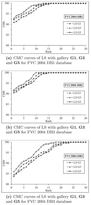
Figure 5.12: CMC curves of LS with the different number of enrolled samples for the different databases.

Table 5.3: HR, PR and searching time (ST) in CS with the different number of enrollments (gallery G1, G3 and G5) into the database

The performance of CS is analyzed with CMS for multiple samples enrollment. The CMC curves are obtained in CS with FVC2004 DB1, DB2, DB3 and DB4 databases with multiple samples enrollment are shown in Fig. 5.13 (a), (b), (c) and (d), respectively. It is observed that CS is produced better performance when more number of samples per fingerprint are enrolled in the database.

 

c) CKS: The results of CKS with the different number of samples enrolled into the database are presented in Table 5.4. It can be shown that rank one HR increases for more number of enrollments without affecting the P R. It can be also observed that CKS requires very less time for large number of samples enrollment.

Figure 5.13: CMC curves of CS with the different number of enrolled samples for the different databases.

Table 5.4: H R, P R and searching time (ST ) in CKS with the different number of enrollments (gallery G1, G3 and G5) into the database

The performance of CKS is also substantiated with CMS. The CMS at the different ranks of cluster kd-tree search with multiple samples enrollment per fingerprint into the database is shown in Fig. 5.14. The results are obtained with the G1, G3 and G5 Gallery sets and P Probe set of all FVC 2004 databases. The CMC curves with this approach for FVC2004 DB1, DB2, DB3 and DB4 are shown in Fig. 5.14 (a), (b), (c) and (d), respectively. It is shown that CKS is also performed better when more number of samples per fingerprint are enrolled in the database.

Figure 5.14: CMC curve of CKS with the different number of enrolled samples for the different databases.

5.6.4 Searching Time

In this section, the searching time complexity of the proposed three searching techniques are calculated. The execution time and the average number of comparisons required in LS, CS and CKS with different number of enrolled samples for the different databases are also reported.

a) LS: Let T_n be the number of index keys from N fingerprints enrolled in the database and each fingerprint has T_p number of index keys on the average. Let T_q be the average number of index keys in the query fingerprint. In LS, T_n × T_q number of comparisons are required to retrieve a set of similar index keys with their identities and T_q log T_q comparisons are required to sort the retrieved identities based on their rank. Thus, the average time complexity of LS (denoted as T_LS) is calculated as in Eq. (5.22).

(5.22)

b) CS: Let T_n index keys are stored in K clusters (rule of thumb of clusters for any unsupervised clustering algorithm [23] for balance between number of clusters and the number of points in a single cluster) and each cluster contains T_k number of index keys on the average. Thus, T_q × K number of comparisons are required to find the matched clusters. A set of T_q × T_k similar index keys with their identities are retrieved for a query fingerprint in Algorithm 5.5. The average number of comparisons required to sort the retrieved identities according to their rank is (T_q × T_k) log(T_q × T_k). Hence, the complexity of the CS can be calculated as in Eq. (5.23).

(5.23)

c) CKS: In CKS, T_q × K number of comparisons are needed to find the matched clusters and T_q log T_k number of comparisons are required to retrieve a set of similar index keys with their identities from the kd-tree for a query fingerprint. The CKS retrieves T_q number of index keys with their identities (see Algorithm 5.6). On the average T_q log T_q number of comparisons are needed to sort the retrieved data according to their rank. Therefore, the complexity of the CKS is calculated in Eq. (5.24).

(5.24)

The execution time (in Intel Core-2 Duo 2.00 GHz processor and 2GB RAM implementation environment) of LS, CS and CKS with different fingerprint databases are shown in Table 5.5. It is observed that the execution time for CKS is less than the other two searching methods. It is also observed that there is no significant changes in the execution time of the CKS when the number of enrolled sample increases. On the other hand, the execution time rapidly increases for LS and CS for enrollment of multiple samples. The average number of comparisons required for LS, CS and CKS are shown in Table 5.5. Hence, it may be concluded that CKS requires the least number of comparisons to retrieve and rank the similar identities for a given query.

Table 5.5: Execution time and average number of comparisons required in LS, CS and CKS with the different number of enrolled samples (ES)

5.6.5 Memory Requirements

In this approach, each value of an index key requires 4 bytes memory. There are 8 key values in the each index key and one identity field is required for each index key. 2¹⁶ identities can be stored with 2 bytes identity field. Hence, 34 bytes is required to store an index along with identity in linear index space. In clustered index space, the memory is needed to store the cluster centroid additional to the linear index space. Each cluster centroid requires 32 bytes memory and 2 bytes memory for cluster id. On the other hand, in clustered kd-tree index space, it is needed to store the cluster centroid and the kd-trees for all clusters. Similar to the clustered index space, each cluster centroid requires 32 bytes memory and 2 bytes memory for cluster id. A single node of kd-tree requires 46 bytes memory. Table 5.6 shows the memory requirements to store different number of fingerprints for different databases for linear, cluster and clustered kd-tree index spaces.

Bibliography

- [1] FLANN - Fast Library for Approximate Nearest Neighbors. URL http://www.cs.ubc.ca/~mariusm/index.php/FLANN/FLANN . (Accessed on May, 2012).
- [2] FVC2004. FVC2004: the Third International Fingerprint Verification Competition. URL http://bias.csr.unibo.it/fvc2004/databases.asp . (Accessed on December, 2011).
- [3] SFinGe. Synthetic Fingerprint Generator. URL http://bias.csr.unibo.it/research/biolab/sfinge.html . (Accessed on January, 2012).
- [4] NIST Special Database 4. NIST 8-Bit Gray Scale Images of Fingerprint Image Groups(FIGS), 1992. URL http://www.nist.gov/srd/nistsd4.cfm . (Accessed on January, 2012).
- [5] S. Arya and D. M. Mount. Algorithms for Fast Vector Quantization. In Proceedings of DCC ’93: Data Compression Conference, pages 381–390, Snowbird, UT, 1993.
- [6] G. Bebis, T. Deaconu, and M. Georgiopoulos. Fingerprint Identification using Delaunay Triangulation. In Proceedings of the IEEE International Conference on Intelligence, Information, and Systems , pages 452–459, Bethesda, USA, October-November 1999. doi: http://dx.doi.org/10.1109/ICIIS.1999.810315.
- [7] J. L. Bentley. Multidimensional Binary Search Trees Used for Associative Searching. Communications of the ACM, 18(9):509–517, 1975. ISSN 0001-0782. doi: http://dx.doi.org/10.1145/361002.361007 .
- [8] B. Bhanu and X. Tan. Fingerprint Indexing Bsed on Novel Features of Minutiae Triplets. IEEE Transactions on Pattern Analysis and Machine Intelligence, 25(5):616–622, 2003. ISSN 0162-8828.
- [9] R. Cappelli. Fast and Accurate Fingerprint Indexing Based on Ridge Orientation and Frequency. IEEE Transactions on Systems, Man, and Cybernetics, Part B: Cybernetics, 41(6):1511–1521, 2011.
- [10] R. Cappelli, A. Lumini, D. Maio, and D. Maltoni. Fingerprint Classification by Directional Image Partitioning. IEEE Transactions on Pattern Analysis and Machine Intelligence, 21(5):402–421, 1999.
- [11] R. Cappelli, D. Maio, and D. Maltoni. Synthetic Fingerprint-Database Generation. In Proceedings of the 16th International Conference on Pattern Recognition, volume 3, pages 744–747, QC, Canada, August 2002.
- [12] R. Cappelli, M. Ferrara, and D. Maltoni. Fingerprint Indexing Based on Minutia Cylinder-Code. IEEE Transactions on Pattern Analysis and Machine Intelligence, 33(5):1051–1057, 2011.
- [13] A. Chatterjee, S. Mandal, G. M. A. Rahaman, and A. S. M. Arif. Fingerprint Identification and Verification System by Minutiae Extraction using Artificial Neural Network. International Journal of Computer and Information Technology (IJCIT), 1(1):12–16, 2010.
- [14] R. C. Gonzalez and R. E. Woods. Digital Image Processing. Prentice Hall, 2nd edition, 2002.
- [15] Z. Guo and R. W. Hall. Parallel Thinning with Two-subiteration Algorithms. Communications of the ACM, 32(3):359–373, 1989.
- [16] L. Hong, Y. Wan, and A. Jain. Fingerprint Image Enhancement: Algorithm and Performance Evaluation. IEEE Transactions on Pattern Analysis and Machine Intelligence, 20(8):777–789, 1998. ISSN 0162-8828.
- [17] A. K. Jain, A. Ross, and S. Prabhakar. An Introduction to Biometric Recognition. IEEE Transactions on Circuits and Systems for Video Technology, 14(1):4–20, 2004.
- [18] X. Jiang, M. Liu, and A. C. Kot. Fingerprint Retrieval for Identification. IEEE Transactions on Information Forensics and Security , 1(4):532–542, 2006.
- [19] X. Liang, A. Bishnu, and T. Asano. A Robust Fingerprint Indexing Scheme using Minutia Neighborhood Structure and Low-Order Delaunay Triangles. IEEE Transactions on Information Forensics and Security, 2(4):721–733, 2007.
- [20] M. Liu, X. Jiang, and A. C. Kot. Fingerprint Retrieval by Complex Filter Responses. In Proceedings of the 18th International Conference on Pattern Recognition, volume 1, pages 1042–1045, Hong Kong, China, August 2006.
- [21] M. Liu, X. Jiang, and A.C. Kot. Efficient Fingerprint Search Based on Database Clustering. Pattern Recognition, 40(6):1793–1803, June 2007.
- [22] D. Maio, D. Maltoni, R. Cappelli, J. L. Wayman, and A. K. Jain. FVC2004: Third Fingerprint Verification Competition. In Proceedings of the International Conference on Biometric Authentication , pages 1–7, Hong Kong, China, July 2004.
- [23] K. V. Mardia, J. T. Kent, and J. M. Bibby. Multivariate Analysis. Academic Press, 1980.
- [24] R. M. McCabe and E. M. Newton. Information Technology: American National Standard for Information Systems - Data Format for the Interchange of Fingerprint, Facial, & Other Biometric Information - Part 1. ANSI/NIST-ITL 1-2007 Revision of ANSI/NIST-ITL 1-2000, 2007.
- [25] B. M. Mehtre. Fingerprint Image Analysis for Automatic Identification. Machine Vision and Applications, 6(2-3):124–139, 1993. doi: 10.1007/BF01211936.
- [26] M. Muja and D. G. Lowe. Fast Approximate Nearest Neighbors with Automatic Algorithm Configuration. In Proceedings of the International Conference on Computer Vision Theory and Applications (VISAPP’09), pages 331–340, 2009.
- [27] A. Ross and R. Mukherjee. Augmenting Ridge Curves with Minutiae Triplets for Fingerprint Indexing. In Proceedings of the SPIE Conference on Biometric Technology for Human Identification IV, volume 6539, pages 65390C–65390C–12, Orlando, USA, April 2007.
- [28] R. Thai. Fingerprint Image Enhancement and Minutiae Extraction. Honours Programme Report, School of Computer Science and Software Engineering, The University of Western Australia, 2003. URL http://www.csse.uwa.edu.au/~pk/studentprojects/raymondthai/RaymondThai.pdf . (Accessed on June, 2011).
- [29] C. J. Watson and C. L. Wilson. NIST Special Database 4, Fingerprint Database. Technical report, National Institute of Standards and Technology, 1992.
- [30] Y. Zhang, J. Tian, K. Cao, P. Li, and X. Yang. Improving Efficiency of Fingerprint Matching by Minutiae Indexing. In Proceedings of the 19th International Conference on Pattern Recognition, pages 1–4, Tampa, FL, December 2008.