
Overview
By the end of this chapter, you will be able to, apply machine learning algorithms to solve different problems; compare, contrast, and apply different types of machine learning algorithms, including linear regression, logistic regression, decision trees, random forests, Naive Bayes, and AdaBoost; analyze overfitting and implement regularization; work with GridSearchCV and RandomizedSearchCV to adjust hyperparameters; evaluate algorithms using a confusion matrix and cross-validation and solve real-world problems using the machine learning algorithms outlined here.
Introduction
Computer algorithms enable machines to learn from data. The more data an algorithm receives, the more capable the algorithm is of detecting underlying patterns within the data. In Chapter 10, Data Analytics with pandas and NumPy, you learned how to view and analyze big data with pandas and NumPy. In this chapter, we will now extend these concepts to building algorithms that learn from data.
Consider how a child learns to identify a cat. Generally speaking, a child learns by having someone point out "That's a cat," "No, that's a dog," and so on. After enough cats and non-cats have been pointed out, the child knows how to identify a cat.
Machine learning implements the same general approach. A convolutional neural network is a machine learning algorithm that distinguishes between images. Upon receiving images labeled cats and non-cats, the algorithm looks for underlying patterns within the pixels by adjusting the parameters of an equation until it finds an equation that minimizes the error.
After the algorithm has selected the best possible equation, given the data it has received, this equation is used to predict future data. When a new image arrives, the new image is placed within the algorithm to determine whether the image is a cat or not.
In this chapter, on machine learning, you will learn how to construct linear regression, logistic regression, decision tree, random forest, Naive Bayes, and AdaBoost algorithms. These algorithms can be used to solve a wide range of problems, from predicting rainfall to detecting credit card fraud and identifying diseases.
Then, you will learn about Ridge and Lasso, two regularized machine learning algorithms that are variations of Linear Regression. You will learn about using regularization and cross-validation to obtain accurate results with data that the algorithm has never seen before.
After learning how to build a machine learning model in scikit-learn through an extended example with linear regression, you will take a similar approach to build models based on k-nearest neighbors, decision trees, and random forests. You will learn how to extend these models with hyperparameter turning, a way of fine-tuning models to meet the specifications of the data at hand.
Next, you will move onto classification problems, where the machine learning model is used to determine whether an email is a spam and whether a celestial object is a planet. All classification problems can be tackled with Logistic Regression, a machine learning algorithm that you will learn about here. In addition, you will solve classification problems with Naïve Bayes, Random Forests, and other types of algorithms. Classification results can be interpreted with a confusion matrix and a classification report, both of which we will explore in-depth.
Finally, you will learn how to implement boosting methods that transform weak learners into strong learners. In particular, you will learn how to implement AdaBoost, one of the most successful machine learning algorithms in history.
To sum it up, after completing this chapter, you will be able to apply multiple machine learning algorithms to solve classification and regression problems. You will be capable of using advanced tools such as a confusion matrix and a classification report to interpret results. You will also be able to refine your models using regularization and hyperparameter tuning. In short, you will have the tools to use machine learning to solve real-world problems, including predicting cost and classifying objects.
Introduction to Linear Regression
Machine learning is the ability of computers to learn from data. The power of machine learning comes from making future predictions based on the data received. Today, machine learning is used all over the world to predict the weather, stock prices, movie recommendations, profits, errors, clicks, purchases, words to complete a sentence, and many more things.
The unparalleled success of machine learning has led to a paradigm shift in the way businesses make decisions. In the past, businesses made decisions based on who had the most influence. But now, the new idea is to make decisions based on data. Decisions are constantly being made about the future, and machine learning is the best tool at our disposal to convert raw data into actionable decisions.
The first step in building a machine learning algorithm is deciding what you want to predict. When looking at a DataFrame, the idea is to choose one column as the target column or predictor column. The target column, by definition, is what the algorithm will be trained to predict.
Recall the Boston Housing dataset introduced in Chapter 10, Data Analytics with pandas and NumPy. The median value of a home is a desirable target column since real estate agents, buyers, and sellers often want to know how much a house is worth. People usually determine this information based on the size of the house, the location, the number of bedrooms, and many other factors.
Here is the Boston Housing DataFrame from Chapter 10, Data Analytics with pandas and NumPy. Each column includes features about houses in the neighborhood, such as crime, the average age of the house, and notably, in the last column, the median value:
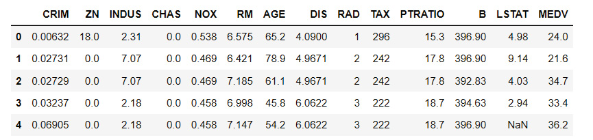
Figure 11.1: Sample from the Boston Housing dataset
You may be wondering what the values CRIM, NOX, and so on mean in the dataset. Don't worry – have a look at the following figure:

Figure 11.2: Dataset value representation
We want to come up with an equation that uses every other column to predict the last column, which will be our target column. What kind of equation should we use? Before we answer this question, let's have a look at a simplified version.
Simplify the Problem
It's often helpful to simplify a problem. What if we take just one column, such as the number of bedrooms, and use it to predict the median house value?
It's clear that the more bedrooms a house has, the more valuable it will be. As the number of bedrooms goes up, so does the house value. A standard way to represent this positive association is with a straight line.
In Chapter 10, Data Analytics with pandas and NumPy, we modeled the relationship between the number of bedrooms and the median house value with the linear regression line, as shown in Figure 11.3:
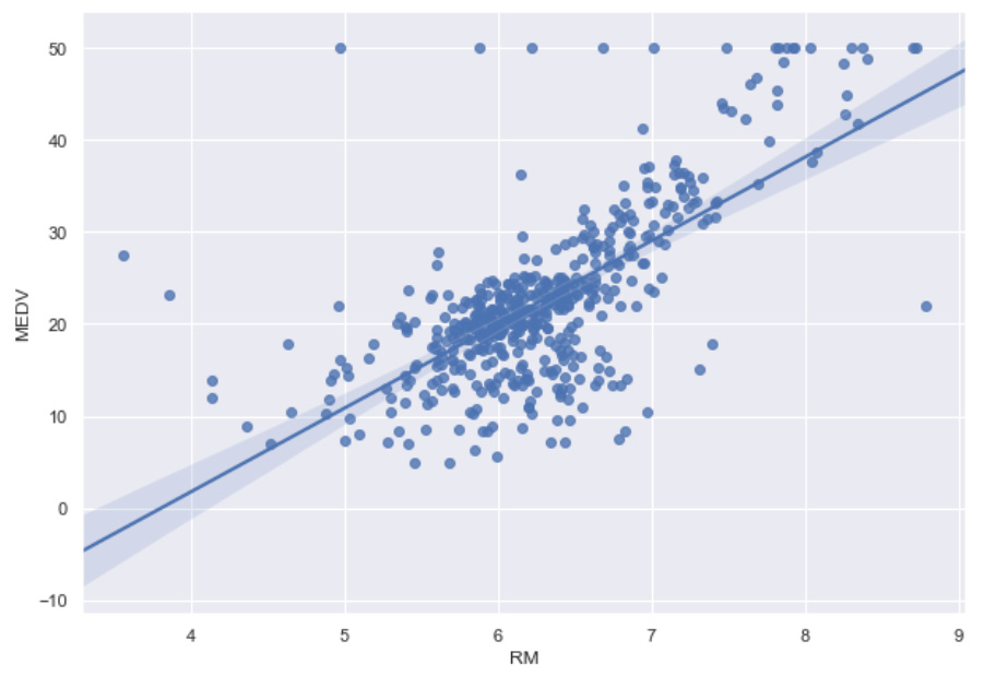
Figure 11.3: Linear regression line for the median value and the number of bedrooms
It turns out that linear regression is a very popular machine learning algorithm. Linear regression is worth trying whenever the target column is a continuous value, as in this dataset. The value of a home is generally considered to be continuous. There is technically no limit to how high the cost of a home may be. It could take any value between two numbers, despite often rounding up.
By contrast, if we predict whether a house will sell after one month on the market, the possible answers are yes and no. In this case, the target column is not continuous but binary.
Note
Whenever the target column is binary, linear regression will not produce strong results.
From One to N-Dimensions
Dimensionality is an important concept in machine learning. In math, it's common to work with two dimensions, x, and y, in the coordinate plane. In physics, it's common to work with three dimensions, the x, y, and z axes. When it comes to spatial dimensions, three is the limit because we live in a three-dimensional universe. In mathematics, however, there is no restriction on the number of dimensions we can use theoretically. In superstring theory, 12 or 13 dimensions are often used. In machine learning, however, the number of dimensions is often the number of predictor columns.
There is no need to limit ourselves to one-dimension with linear regression. Additional dimensions – in this case, additional columns – will give us more information about the median house value and make our model more valuable.
In one-dimensional linear regression, the slope-intercept equation is y = mx + b, where y is the target column, x is the input, m is the slope, and b is the y-intercept. This equation is now extended to an arbitrary number of dimensions using Y = MX + B, where Y, M, and X are vectors of arbitrary length. Instead of the slope, M is referred to as the weight.
Note
It's not essential to comprehend the linear algebra behind vector mathematics to run machine learning algorithms; however, it is essential to comprehend the underlying ideas. The underlying idea here is that linear regression can be extended to an arbitrary number of dimensions.
In the Boston Housing dataset, the linear regression model will select weights for each of the columns. In order to predict the median house value for each row (our target column), the weights will be multiplied by the column entries and then summed to get as close as possible to the value.
We will have a look at how this works in practice.
The Linear Regression Algorithm
Before implementing the algorithm, let's take a brief look at the libraries that we will import and use in our programs:
- pandas – You learned how to use pandas in Chapter 10, Data Analytics with pandas and NumPy. When it comes to machine learning, all data will be handled through pandas. Loading data, reading data, viewing data, cleaning data, and manipulating data all require pandas, so pandas will always be our first import.
- NumPy – NumPy was introduced in Chapter 10, Data Analytics with pandas and NumPy, as well. This will be used for mathematical computations on the dataset. It's always a good idea to import NumPy when performing machine learning.
- LinearRegression – The LinearRegression library should be implemented every time linear regression is used. The LinearRegression library will allow you to build linear regression models and test them in very few steps. Machine learning libraries do the heavy lifting for you. In this case, LinearRegression will place weights on each of the columns and adjust them until it finds an optimal solution to predict the target column, which in our case would be the median house value.
- Mean_squared_error – In order to find optimal values, the algorithm needs a measure to test how well it's doing. Measuring how far the model's predicted value is from the target value is a standard place to start. In order to avoid negatives canceling out positives, we can use mean_squared_error. To compute the mean_squared_error, the prediction of each row is subtracted from the target column or actual value, and the result is squared. Each result is summed, and the mean is computed. Finally, taking the square root keeps the units the same.
- Train_test_split – Python provides train_test_split to split data into a training set and a test set. Splitting the data into a training set and test set is essential because it allows users to test the model right away. Testing the model on data the machine has never seen before is the most important part of building the model because it shows how well the model will perform in the real world.
Most of the data is included in the training set because more data leads to a more robust model. A smaller portion – around 20% – is held back for the test set. The 80-20 split is the default, though you may adjust it as you see fit. The model is optimized on the training set, and after completion, it is scored against the test set.
These libraries are a part of scikit-learn. scikit-learn has a wealth of excellent online resources for beginners. See https://scikit-learn.org/stable/ for more information.
Exercise 145: Using Linear Regression to Predict the Accuracy of the Median Values of Our Dataset
The goal of this exercise is to build a machine learning model using linear regression. Your model will predict the median value of Boston houses and, based on this, we will come to a conclusion about whether the value is optimal or not.
This exercise will be performed on a Jupyter Notebook.
Note
To proceed with the exercises in the chapter, you will need the scikit-learn library that is mentioned in the Preface.
- Open a new notebook file.
- Now, import all the necessary libraries, as shown in the following code snippet:
import pandas as pd
import numpy as np
from sklearn.linear_model import LinearRegression
from sklearn.metrics import mean_squared_error
from sklearn.model_selection import train_test_split
Now that we have imported the libraries, we will load the data.
- Load the dataset and view the DataFrames to look at the first five rows:
# load data
housing_df = pd.read_csv('HousingData.csv')
housing_df.head()
Recall that, as mentioned in Chapter 10, Data Analytics with pandas and NumPy, housing_df = pd.read_cs('HousingData.csv') will read the CSV file in parentheses and store it in a DataFrame called housing_df. Then, housing_df.head() will display the first five rows of the housing_df DataFrame by default.
You should get the following output:
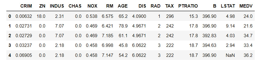
Figure 11.4: Output with the dataset displayed
- Next, enter the following code to clean the dataset of null values using .dropna():
# drop null values
housing_df = housing_df.dropna()
In Chapter 10, Data Analytics with pandas and NumPy, we cleared the null values by counting them and comparing them to measures of central tendency. In this chapter, however, we will use a swifter approach in order to expedite testing for machine learning. The housing_df.dropna() code will drop all null values from the housing_df DataFrame.
Now that the data is clean, it's time to prepare our X and y values.
- Now, declare the X and y variables, where you use X for the predictor columns and y for the target column:
# declare X and y
X = housing_df.iloc[:,:-1]
y = housing_df.iloc[:, -1]
The target column is MEDV, which is the median value of the Boston house prices. The predictor columns include every other column. The standard notation is to use X for the predictor columns and y for the target column.
Since the last column is the target column, which is y, it should be eliminated from the predictor column, that is, X. We can achieve this split by indexing.
- Now we build the actual linear regression model.
Although many machine learning models are incredibly sophisticated, they can be built using very few lines of code. In this case, it takes three steps. We are going to build a model that will predict the median house value given all of the input columns.
The first line uses train_test_split() to split X and y, the predictor and target columns, into training and test sets. The model will be built using the training set.
Split X and y into training and test sets as follows:
#Create training and test sets
X_train, X_test, y_train, y_test = train_test_split(X, y, test_size = 0.2)
test_size = 0.2 reflects the percentage of rows held back for the test set. This is the default setting and does not need to be added explicitly. It is presented so that you know how to change it.
Note
The output values may differ from the values mentioned in the book. We have chosen not use a random seed so that you can get accustomed to diverse outputs.
Next, create an empty LinearRegression() model, as shown in the following code snippet:
#Create the regressor: reg
reg = LinearRegression()
Finally, we fit the model to the data using the .fit() method:
#Fit the regressor to the training data
reg.fit(X_train, y_train)
The parameters are X_train and y_train, which is the training set that we have defined. reg.fit(X_train, y_train) is where machine learning actually happens. In this line, the LinearRegression() model adjusts itself to the training data. The model keeps changing weights, according to the machine learning algorithm, until the weights minimize the error.
You should get the following output:

Figure 11.5: Output when the model adjusts itself to the training data
At this point, reg is a machine learning model with specified weights. There is one weight for each X column. These weights are multiplied by the entry in each row to get as close as possible to the target column, y, which is the median house value.
- Now, find how accurate the model is. Here, we can test it on unseen data:
# Predict on the test data: y_pred y_pred = reg.predict(X_test)
To make a prediction, we implement a method, .predict(). This method takes specified rows of data as the input and produces the corresponding predicted values as the output. The input is X_test, the X-values that were held back for our test set. The output is the predicted y-values.
- We can now test the prediction by comparing the predicted y-values, which is y_pred, to the actual y-values, which is y_test, as shown in the following code snippet:
# Compute and print RMSE
rmse = np.sqrt(mean_squared_error(y_test, y_pred))
print("Root Mean Squared Error: {}".format(rmse))
The error, the difference between the two np.array, may be computed as mean_squared_error. We take the square root of the mean squared error to keep the same units as the target column.
You should get the following output:

Figure 11.6: Output on the accuracy of the dataset model
Note that there are other errors to choose from. The square root of mean_squared_error is a standard choice with linear regression. rmse, short for "root mean squared error," will give us the error of the model on the test set.
A root mean squared error of 5.56 means that, on average, the machine learning model predicts values approximately 5.56 units away from the target value, which is not bad in terms of accuracy. Since the median value (from 1980) is in the thousands, the predictions are about 5.56 thousand off. Lower errors are always better, so we will see if can improve the error going forward.
In this very first exercise, we were able to load our dataset, clean it, and use linear regression, and we were able to train the model to make predictions and find out exactly how accurate it is.
Linear Regression Function
In the first exercise, you were able to see how accurate your Boston Housing median value predictions were. What if you enter the entire code in a function and then run it multiple times? Will you get different results?
You do this as shown in the following example using the same Boston Housing dataset.
Let's put all the machine learning code in a function and run it again.
def regression_model(model):
# Create training and test sets
X_train, X_test, y_train, y_test = train_test_split(X, y, test_size = 0.2)
# Create the regressor: reg_all
reg_all = model
# Fit the regressor to the training data
reg_all.fit(X_train, y_train)
# Predict on the test data: y_pred
y_pred = reg_all.predict(X_test)
# Compute and print RMSE
rmse = np.sqrt(mean_squared_error(y_test, y_pred))
print("Root Mean Squared Error: {}".format(rmse))
Now run the function multiple times to see the results:
regression_model(LinearRegression())
You should get the following output:
Root Mean Squared Error: 4.085279539934423
Now, run the function once again:
regression_model(LinearRegression())
You should get the following output:
Root Mean Squared Error: 4.317496624587608
And finally, run it one more time:
regression_model(LinearRegression())
You should get the following output:
Root Mean Squared Error: 4.7884343211684435
This is troublesome, right? The score is always different. Your scores are also likely to differ from ours.
The scores are different because we are splitting the data into a different training set and test set each time, and the model is based on different training sets. Furthermore, it's being scored against a different test set.
In order for machine learning scores to be meaningful, we want to minimize fluctuation and maximize accuracy. We will see how to do this in the next section.
Cross-Validation
In cross-validation, also known as CV, the training data is split into five folds (any number will do, but five is standard). The machine learning algorithm is fit on one fold at a time and tested on the remaining data. The result is five different training and test sets that are all representative of the same data. The mean of the scores is usually taken as the accuracy of the model.
Note
Five is only one suggestion. Any natural number may be used.
Cross-validation is a core tool for machine learning. Mean test scores on different folds will always be more reliable than one mean test score on the entire set, which we performed in the first exercise. When examining one test score, there is no way of knowing whether it is low or high. Five test scores give a better picture of the accuracy of the model.
Cross-validation can be implemented in a variety of ways. A standard approach is to use cross_val_score, which returns an array of scores for each fold; cross_val_score breaks X and y into the training set and test set for you.
Let's modify our regression machine learning function to include cross_val_score in the following exercise.
Exercise 146: Using the cross_val_score Function to Get Accurate Results on the Dataset
The goal of this exercise is to use cross-validation to obtain more accurate machine learning results from the dataset compared to the previous exercise.
- Continue using the same Jupyter Notebook from Exercise 145, Using Linear Regression to Predict the Accuracy of the Median Values of Our Dataset.
- Now, import cross_val_score:
from sklearn.model_selection import cross_val_score
- Define the regression_model_cv function, which takes a fitted model as one parameter. The k = 5 hyperparameter gives the number of folds. Enter the code shown in the following code snippet:
def regression_model_cv(model, k=5):
scores = cross_val_score(model, X, y, scoring='neg_mean_squared_ error', cv=k)
rmse = np.sqrt(-scores)
print('Reg rmse:', rmse)
print('Reg mean:', rmse.mean ())
In sklearn, the scoring options are sometimes limited. Since mean_squared_error is not an option for cross_val_score, we choose the neg_mean_squared_error. cross_val_score takes the highest value by default, and the highest negative mean squared error is 0.
- Use the regression_model_cv function on the LinearRegression() model defined in the previous exercise:
regression_model_cv(LinearRegression())
You may get something similar to the following output:
Reg rmse: [3.26123843 4.42712448 5.66151114 8.09493087 5.24453989]
Reg mean: 5.337868962878373
- Use the regression_model_cv function on the LinearRegression() model with 3 folds and then 6 folds, as shown in the following code snippet, for 3 folds:
regression_model_cv(LinearRegression(), k=3)
You may get something similar to the following output:
Reg rmse: [ 3.72504914 6.01655701 23.20863933]
Reg mean: 10.983415161090695
- Now, test the values for 6 folds:
regression_model_cv(LinearRegression(), k=6)
You may get something similar to the following output:
Reg rmse: [3.23879491 3.97041949 5.58329663 3.92861033 9.88399671 3.91442679]
Reg mean: 5.08659081080109
You have found out that there is a large discrepancy between the number of folds. One reason is that we have a reasonably small dataset to begin with. In the real world, with a huge amount of data, this generally does not make a huge difference to the results when we compare results with different folds.
Regularization: Ridge and Lasso
Regularization is an important concept in machine learning; it's used to counteract overfitting. In the world of big data, it's easy to overfit data to the training set. When this happens, the model will often perform badly on the test set as indicated by mean_squared_error, or some other error.
You may wonder why a test set is kept aside at all. Wouldn't the most accurate machine learning model come from fitting the algorithm on all the data?
The answer, generally accepted by the machine learning community after years of research and experimentation, is probably not.
There are two main problems with fitting a machine learning model on all the data:
- There is no way to test the model on unseen data. Machine learning models are powerful when they make good predictions on new data. Models are trained on known results, but they perform in the real world on data that has never been seen before. It's not vital to see how well a model fits known results (the training set), but it's absolutely crucial to see how well it performs on unseen data (the test set).
- The model may overfit the data. Models exist that may fit any set of data points perfectly. Consider the 14 green points in the following diagram. A 14th-degree polynomial exists that fits these points almost perfectly. But it's a poor predictor of the new data. The green line is a much better predictor of the new data. Have a look at the following figure to get a better understanding:
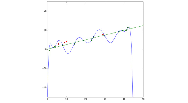
Figure 11.7: Model fitting the data points
There are many models and approaches to counteract overfitting. Let's go over a couple of models now.
Ridge is a simple alternative to linear regression, designed to counteract overfitting. Ridge includes an L2 penalty term (L2 is based on Euclidean Distance) that shrinks the linear coefficients based on their size. The coefficients are the weights, numbers that determine how influential each column is on the output. Larger weights carry greater penalties in Ridge.
Lasso is another regularized alternative to linear regression. Lasso adds a penalty equal to the absolute value of the magnitude of coefficients. This L1 regularization (L1 is taxicab distance.) can eliminate some columns and result in a model that is sparse by comparison.
Let's look at an example to check how Ridge and Lasso perform on our Boston Housing dataset.
In this example, we perform regularization on the dataset using Ridge and Lasso to counteract overfitting. You can continue on the notebook from Exercise 146, Using the cross_val_score Function to Get Accurate Results on the Dataset, to work on this example.
We begin by setting Ridge() as a parameter for regression_model_cv, as shown in the following code snippet:
from sklearn.linear_model import Ridge
regression_model_cv(Ridge())
You should get the following output:
Reg rmse: [3.52479283 4.72296032 5.54622438 8.00759231 5.26861171]
Reg mean: 5.414036309884279
It's not surprising that Ridge has a slightly better score than linear regression. This is because both algorithms use Euclidean distance and the linear regression model is overfitting the data by a slight amount. Your results may be different from ours, however, and the scores are very close.
Another basis of comparison is the worst score of the five. In Ridge, we obtained 8.00759 as the worst score. In linear regression, we obtained 23.20863933 as the worst score. This suggests that 23.20863933 is badly overfitting the training data. In Ridge, this overfitting is compensated.
Now, set Lasso() as the parameter for regression_model_cv:
from sklearn.linear_model import Lasso
regression_model_cv(Lasso())
You should get the following output:
Reg rmse: [4.712548 5.83933857 8.02996117 7.89925202 4.38674414]
Reg mean: 6.173568778640692
Whenever you're trying LinearRegression(), it's always worth trying Lasso and Ridge as well, since overfitting the data is common, and they only actually take a few lines of code to test. Lasso does not perform as well here because the L1 distance metric, taxicab distance, was not used in our model.
Regularization is an essential tool when implementing machine learning algorithms. Whenever you choose a particular model, be sure to research regularization methods to improve your results, as you observed in the preceding example.
Now, let's get to know a developer's doubt. Although we have focused on overfitting the data, underfitting the data is also possible, right? It's less common in the world of big data, though. Underfitting can occur if the model is a straight line, but a higher degree polynomial will fit the data better. By trying multiple models, you are more likely to find optimal results.
So far, you have learned how to implement linear regression as a machine learning model. You have learned how to perform cross-validation to get more accurate results, and you have learned about using two additional models, Ridge and Lasso, to counteract overfitting.
Now that you understand how to build machine learning models using scikit-learn, let's take a look at some different kinds of models that will also work on regression.
K-Nearest Neighbors, Decision Trees, and Random Forests
Are there other machine learning algorithms, besides LinearRegression(), that is suitable for the Boston Housing dataset? Absolutely. There are many regressors in the scikit-learn library that may be used. Regressors are generally considered a class of machine learning algorithms that are suitable for continuous target values. In addition to Linear Regression, Ridge, and Lasso, we can try K-Nearest Neighbors, Decision Trees, and Random Forests. These models perform well on a wide range of datasets. Let's try them out and analyze them individually.
K-Nearest Neighbors
The idea behind K-Nearest Neighbors (KNN) is straightforward. When choosing the output of a row with an unknown label, the prediction is the same as the output of its k-nearest neighbors, where k may be any whole number.
For instance, let's say that k=3. Given an unknown label, we take n columns for this row and place them in n-dimensional space. Then we look for the three closest points. These points already have labels. We assume the majority label for our new point.
KNN is commonly used for classification since classification is based on grouping values, but it can be applied to regression as well. When determining the value of a home, for instance, in our Boston Housing dataset, it makes sense to compare the values of homes in a similar location, with a similar number of bedrooms, a similar amount of square footage, and so on.
You can always choose the number of neighbors for the algorithm and adjust it accordingly. The number of neighbors denoted here is k, which is also called a hyperparameter. In machine learning, the model parameters are derived during training, whereas the hyperparameters are chosen in advance.
Fine-tuning hyperparameters is an essential task to master when building machine learning models. Learning the ins and outs of hyperparameter tuning takes time, practice, and experimentation.
Exercise 147: Using K-Nearest Neighbors to Find the Median Value of the Dataset
The goal of this exercise is to use K-Nearest Neighbors to predict the optimal median value of homes in Boston. We will use the same function, regression_model_cv, with an input of KNeighborsRegressor():
- Continue with the same Jupyter Notebook from the previous Exercise 146.
- Set and import KNeighborsRegressor() as the parameter on the regression_model_cv function:
from sklearn.neighbors import KNeighborsRegressor
regression_model_cv(KNeighborsRegressor())
You should get the following output:
Reg rmse: [ 8.24568226 8.81322798 10.58043836 8.85643441 5.98100069]
Reg mean: 8.495356738515685
K-Nearest Neighbors did not perform as well as LinearRegression(), but it performed respectably. Recall that rmse stands for root mean squared error. So, the mean error is about 8.50 (or 85,000 since the units are ten of thousands of dollars).
We can change the number of neighbors to see if we can get better results. The default number of neighbors is 5. Let's change the number of neighbors to 4, 7, and 10.
- Now, change the n_neighbors hyperparameter to 4, 7, and 10. For 4 neighbors, enter the following code:
regression_model_cv(KNeighborsRegressor(n_neighbors=4))
You should get an output similar to the following:
Reg rmse: [ 8.44659788 8.99814547 10.97170231 8.86647969 5.72114135]
Reg mean: 8.600813339223432
Change n_neighbors to 7:
regression_model_cv(KNeighborsRegressor(n_neighbors=7))
You should get the following output:
Reg rmse: [ 7.99710601 8.68309183 10.66332898 8.90261573 5.51032355]
Reg mean: 8.351293217401393
Change n_neighbors to 10:
regression_model_cv(KNeighborsRegressor(n_neighbors=10))
You should get the following output:
Reg rmse: [ 7.47549287 8.62914556 10.69543822 8.91330686 6.52982222]
Reg mean: 8.448641147609868
The best results so far come from 7 neighbors. But how do we know if 7 neighbors give us the best results? How many different scenarios do we have to check?
Scikit-learn provides a nice option to check a wide range of hyperparameters, which is GridSearchCV. The idea behind GridSearchCV is to use cross-validation to check all possible values in a grid. The value in the grid that gives the best result is then accepted as a hyperparameter.
Exercise 148: K-Nearest Neighbors with GridSearchCV to Find the Optimal Number of Neighbors
The goal of this exercise is to use GridSearchCV to find the optimal number of neighbors for K-Nearest Neighbors to predict the median housing value in Boston. In the previous exercise, if you recall, we used only three neighbor values. Here, we will increase the number using GridSearchCV:
- Continue with the Jupyter Notebook from the previous exercise.
- Import GridSearchCV, as shown in the following code snippet:
from sklearn.model_selection import GridSearchCV
- Now, choose the grid. The grid is the range of numbers – in this case, neighbors – that will be checked. Set up a hyperparameter grid for between 1 and 20 neighbors:
neighbors = np.linspace(1, 20, 20)
We achieve this with np.linspace(1, 20, 20), where the 1 is the first number, the first 20 is the last number, and the second 20 in the brackets is the number of intervals to count.
- Convert floats to int (required by knn):
k = neighbors.astype(int)
- Now, place the grid in a dictionary, as shown in the following code snippet:
param_grid = {'n_neighbors': k}
- Build the model for each neighbor:
knn = KNeighborsRegressor()
- Instantiate the GridSearchCV object – knn_tuned:
knn_tuned = GridSearchCV(knn, param_grid, cv=5, scoring='neg_mean_squared_error')
- Fit knn_tuned to the data using .fit:
knn_tuned.fit(X, y)
- Finally, you print the best parameter results, as shown in the following code snippet:
k = knn_tuned.best_params_
print("Best n_neighbors: {}".format(k))
score = knn_tuned.best_score_
rsm = np.sqrt(-score)
print("Best score: {}".format(rsm))
You should get the following output:

Figure 11.8: Output showing the best score using n_neighbors
In our case, 7 gave the best results. Your results may differ. Now, moving on, let's look at the different types of decision trees and random forests.
Decision Trees and Random Forests
The best way to understand a concept is to relate it to something. You may be familiar with the game Twenty Questions. It's a game in which someone is asked to think of something or someone, perhaps a person. The questioner asks them binary yes or no questions, gradually narrowing down the search in order to determine exactly who they are thinking of.
Twenty Questions is a decision tree. Every time a question is asked, there are two possible branches that the tree may take depending upon the answer. For every new question, new branching occurs, until the branches end at a prediction, called a leaf.
Here is a mini-Decision Tree that predicts whether a Titanic passenger survived:
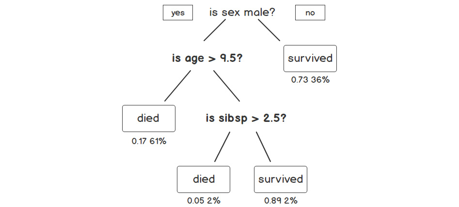
Figure 11.9: Decision tree sample on the Titanic incident
This decision tree starts by determining whether the passenger was male. If the passenger was male, the branch is followed that asks the question was their age greater than 9.5. If the passenger was not male, we reach the end of a branch, and we find out that the probability of survival is 0.73. The other number, 36%, indicates that 36% of the passengers end up at this leaf.
Decision Trees are very good machine learning algorithms, but they are prone to overfitting. A random forest is an ensemble of decision trees. Random forests consistently outperform decision trees because their predictions generalize to data much better. A random forest may consist of hundreds of decision trees.
A random forest is a great machine-learning algorithm to try on almost any dataset. Random forests work well with both regression and classification, and they often perform well out of the box.
Let's try Decision Trees and Random Forests on our data.
Exercise 149: Decision Trees and Random Forests
The goal of this exercise is to use decision trees and random forests to predict median house values in Boston:
- Continue with the same Jupyter Notebook from the previous exercise.
- Use DecisionTreeRegressor() as the input for regression_model_cv.
from sklearn import tree
regression_model_cv(tree.DecisionTreeRegressor())
You should get the following output:
Reg rmse: [3.84098484 5.67885262 7.7328741 6.53263473 5.78903694]
Reg mean: 5.914876645128473
Note
The output values may differ from the values mentioned in the book.
- Use RandomForestRegressor() as the input for regression_model_cv:
from sklearn.ensemble import RandomForestRegressor
regression_model_cv(RandomForestRegressor())
You should get the following output:
Reg rmse: [3.49719743 3.86463108 4.60294622 6.7640934 3.73856719]
Reg mean: 4.493487064599419
As you can see, the random forest regressor gives the best results yet. Let's see if we can improve these results by examining random forest hyperparameters.
Random Forest Hyperparameters
Random forests have a lot of hyperparameters. Instead of going over them all, we will highlight the most important ones:
- n_jobs(default=None): The number of jobs has to do with internal processing. None means 1. It's ideal to set n_jobs = -1 to permit the use of all processors. Although this does not improve the accuracy of the model, it does improve the speed.
- n_estimators(default=10): The number of trees in the forest. The more trees, the better. The more trees, the more RAM is required. It's worth increasing this number until the algorithm moves too slowly. Although 1,000,000 trees may give better results than 1,000, the gain might be small enough to be negligible. A good starting point is 100, and 500 if time permits.
- max_depth(default=None): The max depth of the trees in the forest. The deeper the trees, the more information is captured about the data, but the more prone the trees are to overfitting. When set to the default max_depth of None, there are no limitations, and each tree goes as deep as necessary. The max depth may be reduced to a smaller number of branches.
- min_samples_split(default=2): This is the minimum number of samples required for a new branch or split to occur. This number can be increased to constrain the trees as they require more samples to make a decision.
- min_samples_leaf(default=1): This is the same as min_samples_split, except it's the minimum number of samples at the leaves or the base of the tree. By increasing this number, the branch will stop splitting when it reaches this parameter.
- max_features(default="auto"): The number of features to consider when looking for the best split. The default for regression is to consider the total number of columns. For classification random forests, sqrt is recommended.
Exercise 150: Random Forest Tuned to Improve the Prediction on Our Dataset
The goal of this exercise is to tune a random forest to improve the median house value predictions for Boston:
- Continue with the same Jupyter Notebook from Exercise 149, Decision Trees and Random Forests:
- Set n_jobs = -1 and n_estimators=100 for RandomForestRegressor as the input of regression_model_cv. We can always use n_jobs to speed up the algorithm, and we can increase n_estimators to achieve better results:
regression_model_cv(RandomForestRegressor(n_jobs=-1, n_estimators=100))
You should get the following output:
Reg rmse: [3.29260656 3.61943542 4.83755526 6.49556195 3.76565343]
Reg mean: 4.402162523852732
We could try GridSearchCV on the other hyperparameters to see if we can find a better combination than the defaults, but checking every possible combination of hyperparameters could reach the order of thousands and take way too long.
Note
The output values may differ from the values mentioned in the book.
Sklearn provides RandomizedSearchCV to check a wide range of hyperparameters. Instead of exhaustively going through a list, RandomizedSearchCV will check a set amount of random combinations and return the best results.
- Use RandomizedSearchCV to look for better Random Forest hyperparameters:
from sklearn.model_selection import RandomizedSearchCV
- Set up the hyperparameter grid using max_depth, as shown in the following code snippet:
param_grid = {'max_depth': [None, 10, 30, 50, 70, 100, 200, 400],
'min_samples_split': [2, 3, 4, 5],
'min_samples_leaf': [1, 2, 3],
'max_features': ['auto', 'sqrt']}
- Instantiate the knn regressor:
reg = RandomForestRegressor(n_jobs = -1)
- Instantiate the RandomizedSearchCV object – reg_tuned:
reg_tuned = RandomizedSearchCV(reg, param_grid, cv=5, scoring='neg_mean_squared_error')
- Fit reg_tuned to the data:
reg_tuned.fit(X, y)
- Now, print the tuned parameters and score:
p = reg_tuned.best_params_
print("Best n_neighbors: {}".format(p))
score = reg_tuned.best_score_
rsm = np.sqrt(-score)
print("Best score: {}".format(rsm))
You should get the following output:

Figure 11.10: Output of the tuned parameters and score
Keep in mind that with RandomizedSearchCV, there is no guarantee that the hyperparameters will produce the best results. Although the randomized search did well, it did not perform as well as the defaults with n_jobs = -1 and n_estimators = 100.
- Now, run a random forest regressor with n_jobs = -1 and n_estimators = 500:
# Setup the hyperparameter grid
regression_model_cv(RandomForestRegressor(n_jobs=-1, n_estimators=500))
You should get the following output:
Reg rmse: [3.17315086 3.77060192 4.77587747 6.45161665 3.9681246 ]
Reg mean: 4.427874301108916
Note
Increasing n_estimators every time will produce more accurate results, but the model takes longer to build.
Hyperparameters are a primary key to building excellent machine learning models. Anyone with basic machine learning training can build machine learning models using default hyperparameters. Using GridSearchCV and RandomizedSearchCV to fine-tune hyperparameters to create more efficient models distinguishes advanced users from beginners.
Classification Models
The Boston Housing dataset was great for regression because the target column took on continuous values without limit. There are many cases when the target column takes on one or two values, such as TRUE or FALSE, or possibly a grouping of three or more values, such as RED, BLUE, or GREEN. When the target column may be split into distinct categories, the group of machine learning models that you should try are referred to as classification.
To make things interesting, let's load a new dataset used to detect pulsar stars in outer space. Go to https://packt.live/33SD0IM and click on Data Folder. Then, click on HTRU2.zip.
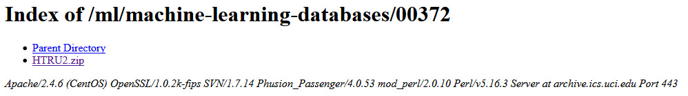
Figure 11.11: Dataset directory on the UCI website
The dataset consists of 17,898 potential pulsar stars in space. But what are these pulsars? Pulsar stars rotate very quickly, so they have periodic light patterns. Radio frequency interference and noise, however, are attributes that make pulsars very hard to detect. This dataset contains 16,259 non-pulsars and 1,639 real pulsars.
Note
The dataset is from Dr. Robert Lyon, University of Manchester, School of Physics and Astronomy, Alan Turing Building, Manchester M13 9PL, United Kingdom, Robert.lyon'@'manchester.ac.uk, 2017.
The columns include information about an integrated pulse profile and a DM-SNR curve. All pulsars produce a unique pattern of emissions, commonly known as their "pulse profile." A pulse profile is similar to a fingerprint, but it is not consistent like a pulsar rotational period. An integrated pulse profile consists of a matrix of an array of continuous values describing the pulse intensity and phase of the pulsar. DM stands for Dispersion Measure, a constant that relates the frequency of light to the extra time required to reach the observer, and SNR stands for Signal to Noise Ratio, which relates how well an object has been measured compared to its background noise.
Here is the official list of columns in the dataset:
- Mean of the integrated profile
- Standard deviation of the integrated profile
- Excess kurtosis of the integrated profile
- Skewness of the integrated profile
- Mean of the DM-SNR curve
- Standard deviation of the DM-SNR curve
- Excess kurtosis of the DM-SNR curve
- Skewness of the DM-SNR curve
- Class
In this dataset, potential pulsars have already been classified as pulsars and non-pulsars by the astronomy community. The goal here is to see if machine learning can detect patterns within the data to correctly classify new potential pulsars that emerge.
The methods that you learn for this topic will be directly applicable to a wide range of classification problems, including spam classifiers, user churn in markets, quality control, product identification, and others.
Exercise 151: Preparing the Pulsar Dataset and Checking for Null Values
The goal of this exercise is to prepare the pulsar dataset for machine learning. The exercises from here on will be on the same notebook file:
- Open a new Jupyter Notebook.
- Import the libraries, load the data, and display the first five rows, as shown in the following code snippet:
import pandas as pd
import numpy as np
df = pd.read_csv('HTRU_2.csv')
df.head()
You should get the following output:
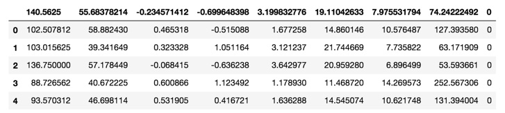
Figure 11.12: The first five rows of the pulsar dataset
Looks interesting, and problematic. Notice that the column headers appear to be another row. It's impossible to analyze data without knowing what the columns are supposed to be, right?
Note that the last column is all 0's in the DataFrame. This suggests that this is the Class column, which is our target column. When detecting the presence of something – in this case, pulsar stars – it's common to use a 1 for positive identification, and a 0 for a negative identification.
Since Class is last in the list, let's assume that the columns are given in the correct order presented in the Attribute Information list. We can also assume that losing the current column headers, a negative identification among 17,898 rows is virtually meaningless. The easiest way forward is simply to change the column headers to match the attribute list.
- Now, change column headers to match the official list and print the first five rows, as shown in the following code snippet:
df.columns = [['Mean of integrated profile', 'Standard deviation of integrated profile',
'Excess kurtosis of integrated profile', 'Skewness of integrated profile',
'Mean of DM-SNR curve', 'Standard deviation of DM-SNR curve',
'Excess kurtosis of DM-SNR curve', 'Skewness of DM-SNR curve', 'Class' ]]
df.head()
You should get the following output:
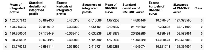
Figure 11.13: Check for null values using df.info() and len(df)
- Now, let's find the info of the dataset using .info():
df.info()
You should get the following output:
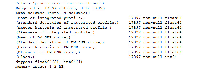
Figure 11.14: Information based on the pulsar dataset
- Finally, use len(df) and match all columns of df.info() with only the non-null entries:
len(df)
You should get the following output:
17897
We know that there are no null values. If there were null values, we would need to eliminate the rows or fill them in by taking the mean, the median, the mode, or another value from the columns.
When it comes to preparing data for machine learning, it's essential to have clean, numerical data with no null values. Further data analysis is often warranted, depending upon the goal at hand. If the goal is simply to try out some models and check them for accuracy, it's fine to go ahead. If the goal is to uncover deep insights about the data, further statistical analysis, as introduced in the previous chapter, is always warranted. Now that we have all this basic information, we can proceed ahead on the same notebook file.
Logistic Regression
When it comes to datasets that classify points, logistic regression is one of the most popular and successful machine learning algorithms. Logistic regression utilizes the sigmoid function to determine whether points should approach one value or the other. As the following diagram indicates, it's a good idea to classify the target values as 0 and 1 when utilizing logistic regression. In the pulsar dataset, the values are already classified as 0s and 1s. If the dataset was labeled as Red and Blue, converting them in advance to 0 and 1 would be essential (you will practice converting categorical to numerical values in the activity at the end of his chapter):
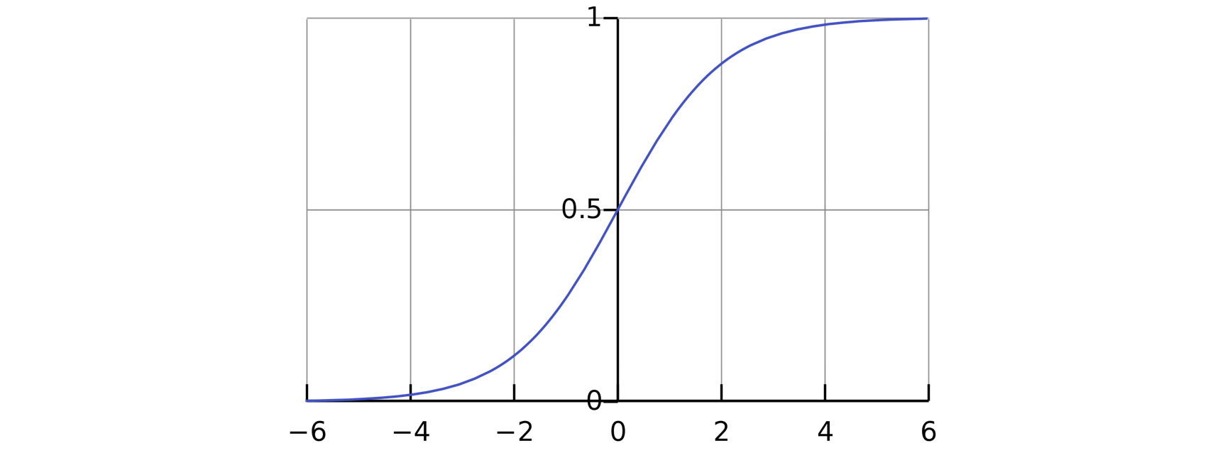
Figure 11.15: Sigmoid curve on a plot
The sigmoid curve in figure 11.14 approaches 1 from the left and 0 from the right, without ever reaching 0 or 1. In this respect, 0 and 1 function as horizontal asymptotes. Basically, every positive x value is given an output of 1, and every negative x value is given an output of 0. Furthermore, the higher up the graph, the higher the probability of a 1, and the lower down the graph, the higher the probability of 0.
Let's see how logistic regression works in action by using a similar function as before.
By default, classifiers use percentage accuracy as the score output.
Exercise 152: Using Logistic Regression to Predict Data Accuracy
The goal of this exercise is to use logistic regression to predict the classification of pulsar stars:
- Import LogisticRegression:
from sklearn.model_selection import cross_val_score
from sklearn.linear_model import LogisticRegression
- Set up matrices X and y to store the predictors and response variables, respectively:
X = df.iloc[:, 0:8]
y = df.iloc[:, 8]
- Write a classifier function that takes a model as its input:
def clf_model(model):
- Create the clf classifier, as shown in the following code snippet:
clf = model
scores = cross_val_score(clf, X, y)
print('Scores:', scores)
print('Mean score:', scores.mean())
- Run the clf_model function with LogisticRegression() as the input:
clf_model(LogisticRegression())
You should get the following output:
Figure 11.16: Mean score using logistic regression
These numbers represent accuracy. A mean score of 0.977706 means that the logistic regression model is classifying 97.8% of pulsars correctly.
Logistic regression is very different than linear regression. Logistic regression uses the sigmoid function to classify all instances into one group or the other. Generally speaking, all cases that are above 0.5 are classified as a 1, and all cases that fall below 0.5 are classified as a 0, with decimals that are close to 1 more likely to be a 1, and decimals that are close to 0 more likely to be a 0. Linear regression, by contrast, finds a straight line that minimizes the error between the straight line and the individual points. Logistic regression classifies all points into two groups; all new points will fall into one of these groups. By contrast, linear regression finds a line of best fit; all new points may fall anywhere on the line and take on any value.
Other Classifiers
There are other classifiers that we can try, including K-Nearest Neighbors (KNN), Decision Trees, Random Forests, and Naive Bayes.
We used KNN, Decision Trees, and Random Forests as regressors before. This time, we need to implement them as classifiers. For instance, there is RandomForestRegressor, and there is RandomForestClassifier. Both are random forests, but they are implemented differently to meet the output of the data. Recall that classifiers have an output of two or more end values, whereas regression has an output of continuous values. The general setup is the same, but the output is different. In the next section, we will have a look at Naive Bayes.
Naive Bayes
Naive Bayes is a model based on Bayes' theorem, a famous probability theorem based on a conditional probability that assumes independent events. Similarly, Naive Bayes assumes independent attributes or columns. The mathematical details of Naive Bayes are beyond the scope of this book, but we can still apply it to our dataset.
There is a small family of machine learning algorithms based on Naive Bayes. The one that we will use here is GaussianNB. Gaussian Naïve Bayes assumes that the likelihood of features is Gaussian. Other options that you may consider trying include MultinomialNB, used for multinomial distributed data (such as text), and ComplementNB, an adaptation of MultinomialNB that is used for imbalanced datasets.
Let's try Naive Bayes, in addition to the KNN, Decision Tree, and Random Forest classifiers mentioned previously.
Exercise 153: Using GaussianNB, KneighborsClassifier, DecisionTreeClassifier, and RandomForestClassifier to Predict Accuracy in Our Dataset
The goal of this exercise is to predict pulsars using a variety of classifiers, including GaussianNB, KneighborsClassifier, DecisionTreeClassifier, and RandomForestClassifier.
- Begin this exercise on the same notebook file from the previous exercise.
- Run the clf_model function with GaussianNB() as the input:
from sklearn.naive_bayes import GaussianNB
clf_model(GaussianNB())
You should get the following output:

Figure 11.17: Mean score using GaussianNB
- Now, run the clf_model function with KNeighborsClassifier() as the input:
from sklearn.neighbors import KNeighborsClassifier
clf_model(KNeighborsClassifier())
You should get the following output:

Figure 11.18: Mean score using KNeighborsClassifier
- Run the clf_model function with DecisionTreeClassifier() as the input:
from sklearn.tree import DecisionTreeClassifier
clf_model(DecisionTreeClassifier())
You should get the following output:

Figure 11.19: Mean score using DecisionTreeClassifier
Note
The output values may differ from the values mentioned in the book.
- Run the clf_model function with RandomForestClassifier() as the input:
from sklearn.ensemble import RandomForestClassifier
clf_model(RandomForestClassifier())
You should get the following output:

Figure 11.20: Mean score using RandomForestClassifier
All classifiers have achieved between 94% and 98% accuracy. It's unusual for this many classifiers to all perform this well. There must be clear patterns within the data, or something is going on behind the scenes.
You may also wonder how to know when to use these classifiers. The bottom line is that whenever you have a classification problem, meaning that the data has a target column with a finite number of options, such as three kinds of wine, most classifiers are worth trying. Naive Bayes is known to work well with text data, and random forests are known to work well generally. New machine learning algorithms are often being developed to handle special cases. Practice and research will help to uncover more nuanced cases.
Confusion Matrix
When discussing classification, it's important to know whether the dataset is imbalanced, as we had some doubts about the results from Exercise 153, Using GaussianNB, KneighborsClassifier, DecisionTreeClassifier and RandomForestClassifier to Predict Accuracy in Our Dataset. An imbalance occurs if the majority of data points have one label rather than another.
Exercise 154: Finding the Pulsar Percentage from the Dataset
The goal of this exercise is to count the percentage of pulsars in our dataset. We will use the Class column. Although we have primarily been using df['Class'] as a way to reference a particular column, df.Class will work as well (except in limited cases, such as setting values):
- Begin this exercise on the same notebook you used in the previous exercise.
- Use the count.() method on df.Class to obtain the number of potential pulsars:
df.Class.count()
You should get the following output:

Figure 11.21: Output of the potential pulsars in the dataset
- Use the .count() method on df[df.Class == 1] to obtain the number of actual pulsars:
df[df.Class == 1].Class.count()
You should get the following output:

Figure 11.22: Output of the total actual pulsars in the dataset
- Divide step 2 by step 1 to obtain the percentage of pulsars:
df[df.Class == 1].Class.count()/df.Class.count()
You should get the following output:
Figure 11.23: Output showing the percentage of pulsars
The results show that 0.09158 or 9% of the data are pulsars. The other 91% are not pulsars. This means that it's very easy to make a machine learning algorithm in this case with 91% accuracy to predict that every row is not a pulsar.
Imagine that the situation is even more extreme. Imagine that we are trying to detect exoplanets, and our dataset has only classified 1% of the data as exoplanets. This means that 99% are not exoplanets. This also means that it's super easy to develop an algorithm with 99% accuracy! Just claim that everything is not an exoplanet!
The confusion matrix was designed to reveal the truth behind imbalanced datasets:
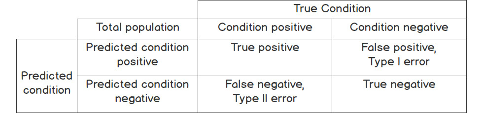
Figure 11.24: Overview of the confusion matrix
As you can see from figure 11.24, the confusion matrix is designed to show you what happened to each of the outputs. Every output will fall into one of four boxes, labeled "True positive," "False positive," "False negative," and "True negative":
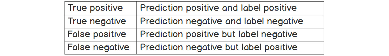
Figure 11.25: Prediction of the confusion matrix based on conditions
Consider the following example. This is the confusion matrix for the decision tree classifier we used earlier. You will see the code to obtain this shortly. First, we want to focus on the interpretation:

Figure 11.26: Confusion matrix
In sklearn, the default order is 0, 1. This means that the zeros or negative values are actually listed first. So, in effect, the confusion matrix is interpreted as follows:
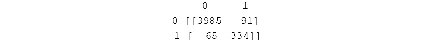
Figure 11.27: Confusion matrix with the default orders
In this particular case, 3,985 non-pulsars have been identified correctly, and 334 pulsars have been identified correctly. The 91 in the upper-right corner indicates that the model classified 91 pulsars incorrectly, and the 65 in the bottom-left corner indicates that 65 non-pulsars were misclassified as pulsars.
It can be challenging to interpret the confusion matrix, especially when positives and negatives do not always line up in the same columns. Fortunately, a classification report may be displayed along with it.
The classification report includes the total number of labels, along with various percentages to help make sense of the numbers and analyze the data.
Here is the classification report with the confusion matrix for the decision tree classifier:
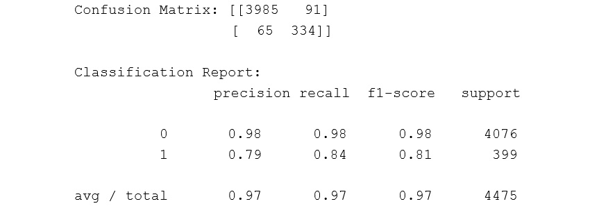
Figure 11.28: Classification report on the confusion matrix
In the classification report, the columns on the two ends are the easiest to interpret. On the far right, support is the number of labels in the dataset. It matches the indexed column on the far left, labeled 0 and 1. Support reveals that there are 4,076 non-pulsars (0s) and 399 pulsars (1s). This number is less than the total because we are only looking at the test set.
Precision is the true positives divided by all the positive predictions. In the case of the zeros, this is 3985 / (3985 + 65), and in the case of the ones, this is 334 / (334 + 91).
Recall is the true positives divided by all the positive labels. For the zeros, this is 3985 / (3985 + 91) and for the ones this is 334 / ( 334 + 65).
The f1-score is the harmonic mean of the precision and recall scores. Note that the f1 scores are very different for the zeros than the ones.
The most important number in the classification report depends on what you are trying to accomplish. Consider the case of the pulsars. Is the goal to identify as many potential pulsars as possible? If so, a lower precision is okay, provided that the recall is higher. Or perhaps an investigation would be expensive. In this case, a higher precision than recall would be desirable.
Exercise 155: Confusion Matrix and Classification Report for the Pulsar Dataset
The goal of this exercise is to build a function that displays the confusion matrix along with the classification report:
- Continue on the same notebook file from the previous exercise.
- Now, import the confusion_matrix and the classification_report libraries:
from sklearn.metrics import classification_report
from sklearn.metrics import confusion_matrix
from sklearn.cross_validation import train_test_split
To use the confusion matrix and classification report, we need a designated test set. We can accomplish this using train_test_split.
- Split the data into a training set and a test set:
X_train, X_test, y_train, y_test = train_test_split(X, y, test_size = 0.25)
Now, build a function called confusion that takes a model as the input and prints the confusion matrix and classification report. The clf classifier should be the output:
def confusion(model):
- Create a model classifier:
clf = model
- Fit the classifier to the data:
clf.fit(X_train, y_train)
- Predict the labels of the y_pred test set:
y_pred = clf.predict(X_test)
- Compute and print the confusion matrix:
print('Confusion Matrix:', confusion_matrix(y_test, y_pred))
- Compute and print the classification report:
print('Classification Report:', classification_report(y_test, y_pred))
return clf
Now let's try the function on our various classifiers.
- Run the confusion() function with LogisticRegression as the input:
confusion(LogisticRegression())
You should get the following output:
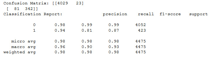
Figure 11.29: Output of the confusion matrix on LogisticRegression
As you can see, the precision of classifying actual pulsars, the 1 in the classification report, is 94%, whereas the total is 98%. Perhaps more significantly, the f1-score, which is the average of the precision and recall scores, is 98% overall, but only 87% for the pulsars, or ones.
- Now, run the confusion() function with KNeighborsClassifier() as the input:
confusion(KNeighborsClassifier())
You should get the following output:
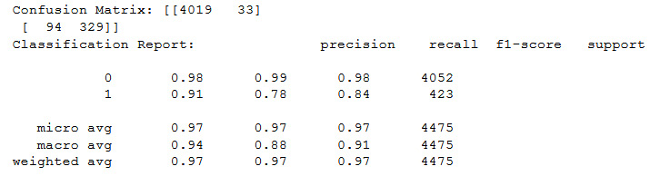
Figure 11.30: Output of the confusion matrix on KNeighborsClassifier
They're all high scores overall, but the 78% recall and 84% f1-score for the pulsars are a little lacking.
- Run the confusion() function with GaussianNB() as the input:
confusion(GaussianNB())
You should get the following output:
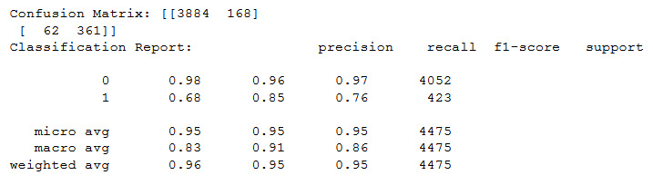
Figure 11.31: Output of the confusion matrix on GaussianNB
In this particular case, the 68% precision of correctly identifying pulsars is not up to par.
- Run the confusion() function with RandomForestClassifer() as the input:
confusion(RandomForestClassifier())
You should get the following output:
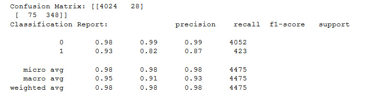
Figure 11.32: Output of the confusion matrix on RandomForestClassifier
We've now finished this exercise, and you can see that, in this case, the f1-score of 87% is the highest that we have seen.
Which classifier would give the best results if we want to detect pulsars? RandomForestClassifier() is great because it has the highest precision and recall for pulsar identification. If the goal is to detect pulsars, RandomForestClassifier is the best bet.
Boosting Methods
Random Forests are a type of bagging method. A bagging method is a machine learning method that aggregates a large sum of machine learning models. In the case of Random Forests, the aggregates are decision trees.
Another machine learning method is boosting. The idea behind boosting is to transform a weak learner into a strong learner by modifying the weights for the rows that the learner got wrong. A weak learner may have an error of 49%, hardly better than a coin flip. A strong learner, by contrast, may have an error rate of 1 or 2 %. With enough iterations, very weak learners can be transformed into very strong learners.
The success of boosting methods caught the attention of the machine learning community. In 2003, Yoav Fruend and Robert Shapire won the 2003 Godel Prize for developing AdaBoost, short for adaptive boosting.
Like many boosting methods, AdaBoost has both a classifier and a regressor. AdaBoost adjusts weak learners toward instances that were previously misclassified. If one learner is 45% correct, the sign can be flipped to become 55% correct. By switching the signs of negatives to positives, the only problematic instances are those that are exactly 50% correct because changing the sign will not change anything. The larger the percentage that is correct, the larger the weight given is given out to sensitive outliers.
Let's see how the AdaBoost classifier performs on our datasets.
Exercise 156: Using AdaBoost to Predict the Best Optimal Values
The goal of this exercise is to predict pulsars and median housing prices in Boston using AdaBoost:
- Begin this exercise on the same notebook you used in the previous exercise.
- Now, import AdaBoostClassifier and use it as the input for clf_model():
from sklearn.ensemble import AdaBoostClassifier
clf_model(AdaBoostClassifier())
You should get the following output:

Figure 11.33: Mean score output using AdaBoostClassifier
As you can see, the AdaBoost classifier gave one of the best results yet. Let's see how it performs on the confusion matrix.
- Use AdaBoostClassifer() as the input for the confusion() function:
confusion(AdaBoostClassifier())
You should get the following output:
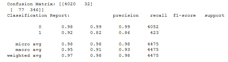
Figure 11.34: Output of the confusion matrix on AdaBoostClassifier
Totals of 98% for precision, recall, and the f1-score are outstanding. The f1-score of the positive pulsar classification, the 1's, is 86%, nearly performing as well as RandomForestClassifier.
Note
Now, head to the notebook file for exercises 146-150 and execute the following steps.
- Set X and y equal to housing_df.iloc[:, :-1] and housing_df.iloc[:, -1]:
X = housing_df.iloc[:,:-1]
y = housing_df.iloc[:, -1]
- Now, import AdaBoostRegressor and use AdaBoostRegressor() as the input for the regression_model_cv function:
from sklearn.ensemble import AdaBoostRegressor
regression_model_cv(AdaBoostRegressor())
You should get the following output:
Figure 11.35: Mean score output using AdaBoostRegressor
It's no surprise that AdaBoost also gives one of the best results on the housing dataset. It has a great reputation for a reason.
AdaBoost is one example of many reputable boosters. XGBoost, and its successor, LightGBM, followed in the footsteps of AdaBoost. They are not part of the sklearn library, however, so we will not implement them in this book.
Activity 25: Using Machine Learning to Predict Customer Return Rate Accuracy
In this activity, you will use machine learning to solve a real-world problem. A bank wants to predict whether customers will return, also known as churn. They want to know which customers are most likely to leave. They give you their data, and they ask you to create a machine-learning algorithm to help them target the customers most likely to leave.
The overview for this activity will be for you to first prepare the data in the dataset, then run a variety of machine learning algorithms that were covered in this chapter to check their accuracy. You will then use the confusion matrix and classification report to help find the best algorithm to identify cases of user churn. You will select one final machine learning algorithm along with its confusion matrix and classification report for your output.
Here are the steps to achieve this goal:
- Download the dataset from https://packt.live/35NRn2C.
- Open CHURN.csv in a Jupyter Notebook and observe the first five rows.
- Check for NaN values and remove any that you find in the dataset.
- In order to use machine learning on all the columns, the predictive column should be in terms of numbers, not 'No' and 'Yes'. You may replace 'No' and 'Yes' with 0 and 1 as follows:
df['Churn'] = df['Churn'].replace(to_replace=['No', 'Yes'], value=[0, 1])
- Set X, the predictor columns, equal to all columns except the first and the last. Set y, the target column, equal to the last column.
- You want to transform all of the predictive columns into numeric columns. This can be achieved as follows:
X = pd.get_dummies(X)
- Write a function called clf_model that uses cross_val_score to implement a classifier. Recall that cross_val_score must be imported.
- Run your function on five different machine learning algorithms. Choose the top three models.
- Build a similar function using the confusion matrix and the classification report that uses train_test_split. Compare your top three models using this function.
- Choose your best model, look at the hyperparameters, and optimize at least one hyperparameter.
You should get an output similar to the following:
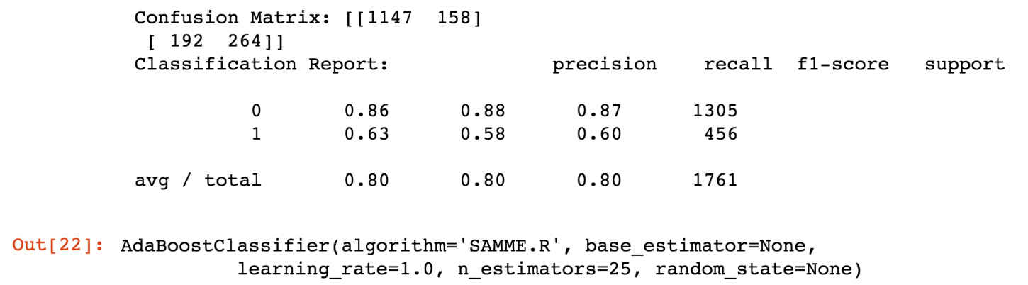
Figure 11.36: Expected confusion matrix output
Note
The solution for this activity is available on page 559.
Summary
In this chapter, you have learned how to build a variety of machine learning models to solve regression and classification problems. You have implemented Linear Regression, Ridge, Lasso, Logistic Regression, Decision Trees, Random Forests, Naive Bayes, and AdaBoost. You have learned about the importance of using cross-validation to split up your training set and test set. You have learned about the dangers of overfitting and how to correct it with regularization. You have learned how to fine-tune hyperparameters using GridSearchCV and RandomizedSearchCV. You have learned how to interpret imbalanced datasets with a confusion matrix and a classification report. You have also learned how to distinguish between bagging and boosting, and precision and recall.
The truth is that you have only scratched the surface of machine learning. In addition to classification and regression, there are many other popular classes of machine learning algorithms, such as recommenders, which are used to recommend what movies or books a user may like based on their preferences and what they have liked before, and unsupervised algorithms, which group data in unpredictable ways.
With this chapter, we come to the end of our journey in this book. We've learned the basics of Python and how to get started from opening a Jupyter Notebook and loading the necessary libraries, to working with lists, dictionaries, and sets; after which, we moved on to visually outputting data using Python, which is an essential part of presenting data. We saw not only how to code in Python, but also how to be Pythonic, which is the smarter way to code in Python. We then covered using unit testing and debugging techniques to handle errors. Lastly, we saw how to learn from big data in this last chapter on machine learning.