
6
Product Recommendation
Product recommendation is essentially a filtering system that aims to anticipate and present the goods that a user would be interested in buying. It is used to generate recommendations that keep users engaged with your product and service and provides relevant suggestions to them. In this chapter, we will learn how to do the following:
- Detect clients who are reducing their sales
- Target clients with personalized product suggestions for products that they are not yet buying
- Create specific product recommendations based on already bought products using market basket analysis and the Apriori algorithm
Let’s determine what will be the requirements to understand the steps and follow the chapter.
This chapter covers the following topics:
- Targeting decreasing returning buyers
- Understanding product recommendation systems
- Using the Apriori algorithm for product bundling
Technical requirements
In order to be able to follow the steps in this chapter, you will need to meet the next requirements:
- Have a Jupyter notebook instance running Python 3.7 and above. You can also use the Google Colab notebook to run the steps if you have a Google Drive account.
- Have an understanding of basic math and statistical concepts.
Targeting decreasing returning buyers
One important aspect of businesses is that recurring customers always buy more than new ones, so it’s important to keep an eye on them and act if we see that they are changing their behavior. One of the things that we can do is identify the clients with decreasing buying patterns and offer them new products that they are not yet buying. In this case, we will look at consumer goods distribution center data to identify these customers with decreasing purchases:
- First, we will import the necessary libraries, which are the following: pandas for data manipulation, NumPy for masking and NaNs handling, and scikit-surprise for collaborative filtering product recommendation.
- We will explore the data to determine the right strategy to normalize the data into the right format.
- Once the data is structured, we will set up a linear regression to determine the clients with a negative slope to identify the ones with decreasing consumption patterns. This information will allow us to create specific actions for these clients and avoid customer churn.
Let’s get started with the following steps:
- Our first stage will be to load these packages and install the scikit-surprise package for collaborative filtering, which is a method to filter out items that a user might like based on the ratings of similar users. It works by linking the behaviors of a smaller set of users with tastes similar to a particular user product recommendations:
import numpy as np
- For readability purposes, we will limit the maximum number of rows to be shown to 20, set the limit of maximum columns to 50, and show the floats with 2 digits of precision:
pd.options.display.precision = 2
- Now we can load the data to be analyzed:
df.head()
In the next figure, we show the historical sales of sold goods by period, details of both the client and product, and the quantity sold:

Figure 6.1: Data of consumer goods transactions
The data consists of buy orders from different clients, for different products and different periods. The data has a period column with information about both the year and the month when the buy was made.
- We can keep exploring the data by taking a look at the columns list:
>>> ['period', 'sub_market', 'client_class', 'division', 'brand','cat', 'product', 'client_code', 'client_name', 'kgs_sold']
- Now, let’s look at the total number of clients to analyze:
>>> 11493
In this case, we have almost 12,000 clients. For the demonstration purposes of this chapter, we will focus on the most important clients, based on the criteria of who are the ones that consume the most.
- Now, we will find the clients that have been reducing sales. We will gauge the information to get the list of clients that have the highest total number of kilograms of products purchased to determine the best customers. We will use the groupby method with the sum by period to get the kilograms bought per client and period:
kgs_by_period = kgs_by_period.groupby(['
kgs_by_period.head()
In the next figure, we can see the total kilograms of goods sold by client and period:
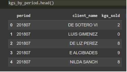
Figure 6.2: Aggregate sum of goods in kg by client and period
- Now that we have the list of total clients, we will characterize them by the number of purchases per period:
unique_clients.head()
In the next DataFrame, we can see the count of purchases by client:
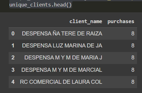
Figure 6.3: Data of users per number of purchases
- Now we will filter top clients by the number of purchases, keeping the ones with at least five purchases of the total 8 periods we have. This limit is arbitrary in this case to find the clients that are mostly regular clients:
unique_clients = unique_clients[unique_clients.purchases>5]
- Now, we can check the total number of clients again:
>>> (7550, 2)
As we can see, most of the clients have more than 5 periods of purchases, so we have reduced around 30% of the total users.
- Now, we will list the total kgs of goods sold in all of the periods, filtering the clients that have less than 5 periods of buys:
kgs_by_client = kgs_by_client[kgs_by_client.client_name.isin(unique_clients.client_name)]
- Now, to get the total number of kgs sold in all of the periods, we will use the groupby method and sort the values in ascending order:
kgs_by_client = kgs_by_client.sort_values([
'total_kgs'],ascending= False)
- As the next step and only for visualization and demonstration, we will limit the clients to the top 25 clients:
kgs_by_client.head()
We can then see the top 25 clients by total kgs:

Figure 6.4: Clients with the highest kgs bought
- Now that we have the information about the top clients in terms of kgs sold, we can create a histogram to understand their consumption patterns. We will be using the plot method to create a bar chart for the pandas Dataframe:
kgs_by_client.plot(kind='bar',x='client',y='total_kgs',figsize=(14,6),rot=90)
This results in the following output:

Figure 6.5: Chart of clients with the highest amount of kgs sold
- To capture the clients that have been decreasing their level of expenditure, we will create a mask that filters all but the top clients, to visualize the kgs bought per client and period:
kgs_by_period = kgs_by_period.sort_values([
kgs_by_period
This is the filtered data after filtering the top clients by weight:

Figure 6.6: Kgs sold by period and client
- Finally, we will pivot the DataFrame for visualization, and we will fill the NaN values with 0 as this is an indication that the client did not buy anything for this period:
dfx = kgs_by_period.pivot(index='period',columns=
dfx
The next DataFrame has the data pivoted and is better encoded for working with machine learning models:
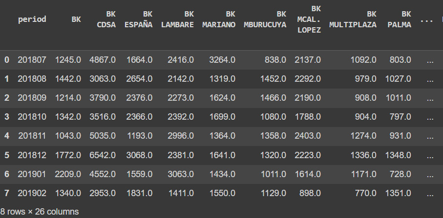
Figure 6.7: Pivoted data
- Now, we can visualize the consumption throughout the periods:
g.legend(loc='center left', bbox_to_anchor=(1, 0.5))
The line plot allows us to see at first glance the clients with the biggest sales:

Figure 6.8: Line plot of kgs sold by client and period
- To identify the curves with a decreasing trend, we will determine the slope and the standard deviation in terms of sales per month. This will allow us to identify the clients with decreasing consumer behavior by looking at the slope as well as to identify users with high consumption variability:
print('Client Name:',client,'; Buy Tendency (Slope):',round(slope,3),'; Common Standard deviation:',round(std_err,3))
We can see in the prints that some of the clients have a negative slope, which indicates that their consumer patterns show a decline in monthly purchases:
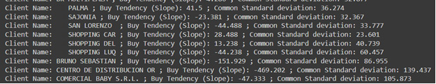
Figure 6.9: Slope of clients buying trends
In this case, the values are shown in absolutes, but it would be even better to show it as a percentage of the median purchase of each client to keep the consistency. You can apply this change and evaluate the difference.
- Next, we will store the results in a DataFrame and use it to visualize the results:
results_df.head()
The DataFrame shows us the clients, along with the parameter estimated by the regression model:

Figure 6.10: Final slope and standard deviation
- Now that our information is neatly structured, we can create a seaborn heatmap to visualize the resulting data more graphically:
sns.heatmap(results_df, annot=True)
This results in the following output:

Figure 6.11: Slope and deviation heatmap
From the data, we can see some clients that show a marked decline in their monthly purchases, and some of them have been increasingly buying more. It is also helpful to look at the standard deviation to find how varying the purchases that this client does are.
Now that we understand the performance of each one of the clients, we can act on the clients with a pattern of declining sales by offering them tailor-made recommendations. In the next section, we will train recommender systems based on the purchase pattern of the clients.
Understanding product recommendation systems
Now that we have identified the customers with decreasing consumption, we can create specific product recommendations for them. How do you recommend products? In most cases, we can do this with a recommender system, which is a filtering system that attempts to forecast and display the products that a user would like to purchase as what makes up a product suggestion. The k-nearest neighbor method and latent factor analysis, which is a statistical method to find groups of correlated variables, are the two algorithms utilized in collaborative filtering. Additionally, with collaborative filters, the system learns the likelihood that two or more things will be purchased collectively. A recommender system’s goal is to make user-friendly recommendations for products in the same way that you like. Collaborative filtering approaches and content-based methods are the two main categories of techniques available to accomplish this goal.
The importance of having relevant products being recommended to the clients is critical, as businesses can personalize client experience with the recommended system by recommending the products that make the most sense to them based on their consumption patterns. To provide pertinent product recommendations, a recommendation engine also enables companies to examine the customer’s past and present website activity.
There are many applications for recommender systems, with some of the most well-known ones including playlist makers for video and audio services, product recommenders for online shops, content recommenders for social media platforms, and open web content recommenders.
In summary, recommendation engines provide personalized, direct recommendations that are based on the requirements and interests of each client. Machine learning is being used to improve online searches as well as it provides suggestions based on a user’s visual preferences rather than product descriptions.
Creating a recommender system
Our first step to train our recommender system is to capture the consumption patterns of the clients. In the following example, we will focus on the products that the customers bought throughout the periods:
dfs = df[['client_name','product']].groupby(['client_name','product']).size().reset_index(name='counts')
dfs =  dfs.sort_values(['counts'],ascending=False)
dfs.head()
This results in the following output:

Figure 6.12: Products bought by client
We will train the recommender with a rating scale between 0 and 1 so we need to scale these values. Now we can see that some clients have consistently bought some products, so we will use the sklearn min max scaler to adjust the scale.
In machine learning, we normalize the data by generating new values, maintaining the general distribution, and adjusting the ratio in the data; normalization prevents the use of raw data and numerous dataset issues. Utilizing a variety of methods and algorithms also enhances the efficiency and accuracy of machine learning models.
The MinMaxScaler from scikit-learn can be applied to scale the variables within a range. It’s important to note that the distribution of the variables should be normal. The original distribution’s shape is preserved by MinMaxScaler making sure that the information present in the original data is not materially altered. Keep in mind that MinMaxScaler does not lessen the significance of outliers and that the resulting feature has a default range of 0 to 1.
Which scaler—MinMaxScaler or StandardScaler—is superior? For features that follow a normal distribution, StandardScaler is helpful. When the upper and lower boundaries are well defined from domain knowledge, MinMaxScaler may be employed (pixel intensities that go from 0 to 255 in the RGB color range).
from sklearn.preprocessing import MinMaxScaler
scaler = MinMaxScaler()
dfs['count_sc'] = scaler.fit_transform(dfs[['counts']])
dfs = dfs.drop(['counts'],axis=1)
Now that we have standardized the values, we can start working on the recommender system. Here, we will be using the SVDpp algorithm, which is an extension of SVD that takes into account implicit ratings. SVD is employed as a collaborative filtering mechanism in the recommender system. Each row in the matrix symbolizes a user, and each column is a piece of merchandise. The ratings that users provide for items make up the matrix’s elements.
The general formula of SVD is:
M=UΣVᵗ
where:
- M is the original matrix we want to decompose, which is the dense matrix of users and products they bought
- U is the left singular matrix (columns are left singular vectors)
- Σ is a diagonal matrix containing singular eigenvalues
- V is the right singular matrix (columns are right singular vectors)
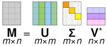
Figure 6.13: Collaborative filtering factorization matrix
The scikit-surprise package efficiently implements the SVD algorithm. Without having to reinvent the wheel, we can quickly construct rating-based recommender systems using the simple-to-use Python module called SurpriseSVD. When utilizing models such as SVD, SurpriseSVD also gives us access to the matrix factors, which enables us to visually see how related the objects in our dataset are:
- We will start by importing the libraries:
from surprise import Reader, Dataset
- Now, we will initiate the reader for which we will set the scale between 0 and 1:
reader = Reader(rating_scale=(0,1))
- Then, we can load the data with the Dataset method from the DataFrame with standardized value counts of products:
data = Dataset.load_from_df(dfs, reader)
- Finally, we can instantiate the SVD algorithm and train it on the data:
algo.fit(data.build_full_trainset())
The training process should take a couple of minutes depending on the hardware specs that you have, but once it is finished, we can start using it to make predictions.
- We will start by taking a particular user and filtering up all the products that they are still not buying to offer them the ones that are more recommended:
prods = [p for p in prods if p not in user_prods]
- Now that we have determined the products that the user is not buying, let’s see how the algorithm rates them to this specific user:
my_recs.append((iid, algo.predict(uid=usr,iid=iid).est))
- The preceding code will iterate over the products in the following data and create a DataFrame with the products that have the highest recommendation value:
dk.head()
The next DataFrame shows us the recommended products for the client:

Figure 6.14: Client-recommended products
- Now that we have determined this for a single user, we can extrapolate this to the rest of the clients. We will keep only the first 20 recommendations, as the number of products is too extensive:
dki_full = pd.concat([dki_full, dk.head(20)])
This script will allow us to loop through our clients and generate a list of recommendations for each one of them. In this case, we are looking into a specific analysis, but this could be implemented into a pipeline delivering these results in real time.
Now we have data that allows us to target each one of our clients with tailor-made product recommendations for products that they are not buying yet. We can also offer products that are complementary to the ones they are already buying, and this is what we will do in the next section.
Using the Apriori algorithm for product bundling
For now, we have focused on clients that are decreasing their purchases to create specific offers for them for products that they are not buying, but we can also improve the results for those that are already loyal customers. We can improve the number of products that they are buying by doing a market basket analysis and offering products that relate to their patterns of consumption. For this, we can use several algorithms.
One of the most popular methods for association rule learning is the Apriori algorithm. It recognizes the things in a data collection and expands them to ever-larger groupings of items. Apriori is employed in association rule mining in datasets to search for several often-occurring sets of things. It expands on the itemsets’ connections and linkages. This is the implementation of the “You may also like” suggestions that you frequently see on recommendation sites are the result of an algorithm.
Apriori is an algorithm for association rule learning and frequent item set mining in relational databases. As long as such item sets exist in the database frequently enough, it moves forward by detecting the frequent individual items and extending them to larger and larger item sets. The Apriori algorithm is generally used with transactional databases that are mined for frequent item sets and association rules using the Apriori method. “Support”, “Lift”, and “confidence” are utilized as parameters, where support is the likelihood that an item will occur, and confidence is a conditional probability. An item set is made up of the items in a transaction. This algorithm uses two steps, “join” and “prune,” to reduce the search space. It is an iterative approach to discovering the most frequent itemsets. In association rule learning, the items in a dataset are identified, and the dataset is expanded to include ever-larger groupings of things.
The Apriori method is a common algorithm used in market basket analysis and is a well-known and widely used association rule algorithm. It aids in the discovery of frequent itemsets in transactions and pinpoints the laws of association between these items.
Performing market basket analysis with Apriori
For this analysis, we will use separate data found in the UCI ML repository (http://archive.ics.uci.edu/ml/datasets/Online+Retail):
- We begin the analysis by importing the packages and loading the data. Remember to install the mlxtend module prior to running this block of code, otherwise, we will have a Module Not Found error:
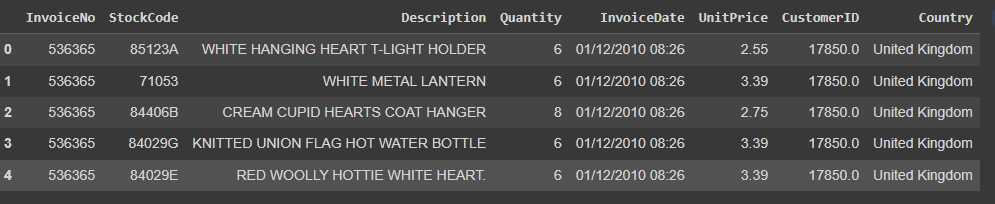
Figure 6.15: Online retail data
This international data collection includes every transaction made by a UK-based, registered non-store internet retailer between December 1, 2010, and December 9, 2011. The company primarily offers one-of-a-kind gifts for every occasion. The company has a large number of wholesalers as clients.
- We begin exploring the columns of the data:
>>> Index(['InvoiceNo', 'StockCode', 'Description', 'Quantity', 'InvoiceDate','UnitPrice', 'CustomerID', 'Country'],dtype='object')
The data contains transactional sales data with information about codes and dates that we will not use now. Instead, we will focus on the description, quantity, and price.

Figure 6.16: Descriptive statistical summary
- In order to assess the categorical variables, we use the describe method focused on object columns in the DataFrame:
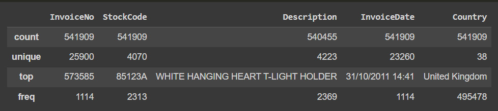
Figure 6.17: Descriptive categorical summary
This information shows us some of the counts for each object column and shows us that the most common country is the UK, as expected.

Figure 6.18: Markets in the data
We can confirm that the vast majority of transactions are in the UK, followed by Germany and France.
- For readability, we will be stripping extra spaces in the description:
data['Description'] = data['Description'].str.strip()
- Now, we will drop rows with NaNs in the invoice number and convert them into strings for categorical treatment:
data['InvoiceNo'] = data['InvoiceNo'].astype('str') - For now, we will focus on noncredit transactions, so we will be dropping all transactions that were done on credit:
data = data[~data['InvoiceNo'].str.contains('C')] - We will begin the analysis by looking at the UK association rules:
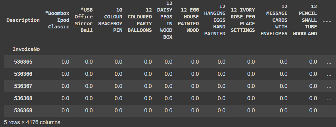
Figure 6.19: UK market basket
We can see the dense matrix of products bought on each invoice.
- We will do the same with the transactions done in France:
basket_fr = basket_fr.set_index('InvoiceNo') - Finally, we will do the same for the data for Germany:
basket_de = basket_de.set_index('InvoiceNo') - Now, we will be defining the hot encoding function to make the data suitable for the concerned libraries as they need discrete values (either 0 or 1):
basket_de = (basket_de>0).astype(int)
- Once we have encoded the results into a one hot encoder, we can start to build the models for each market:
frq_items_uk = apriori(basket_uk, min_support = 0.01, use_colnames = True)
- Once the model is built, we can look at the found association rules for the UK market:
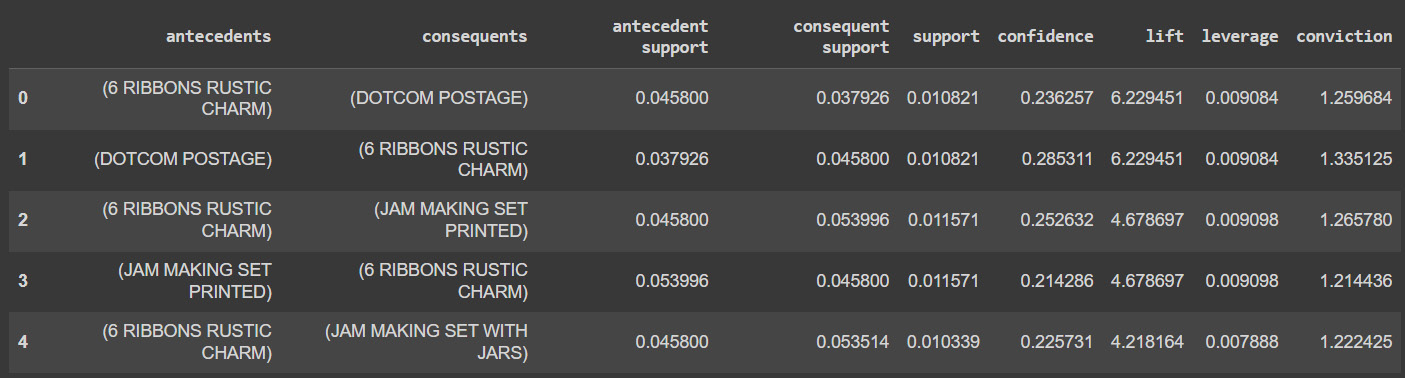
Figure 6.20: UK association rules
If the rules for the UK transactions are examined in more detail, it becomes clear that the British bought variously colored tea plates collectively. This may be due to the fact that the British often enjoy tea very much and frequently collect various colored tea dishes for various occasions.
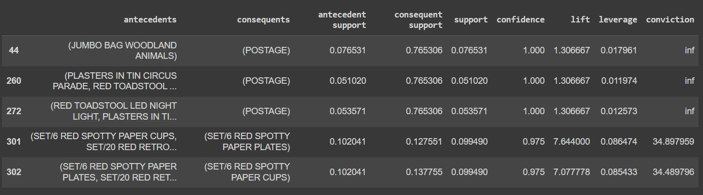
Figure 6.21: France association rules
It is clear from this data that paper plates, glasses, and napkins are frequently purchased together in France. This is due to the French habit of gathering with friends and family at least once every week. Additionally, since the French government has outlawed the use of plastic in the nation, citizens must purchase replacements made of paper.

Figure 6.22: Germany association rules
The preceding data shows us that most of the items are associated with costs of delivery, so it might be an indication that German transactions are mostly made of single items.
Summary
In this chapter, we have learned to identify the clients that have a decreasing number of sales in order to offer them specific product recommendations based on their consumption patterns. We have identified the decreasing sales by looking at the slope in the historical sales in the given set of periods, and we used the SVD collaborative filtering algorithm to create personalized recommendations for products that customers are not buying.
As the next step and to improve the loyalty of existing customers, we have explored the use of the Apriori algorithm to run a market basket analysis and to be able to offer product recommendations based on specific products being bought.
In the next chapter, we will dive into how we identify the common traits of customers that churn in order to complement these approaches with a deeper understanding of our customer churn.