
For clustering music with audio data, the data points are the feature vectors from the audio files. If two points are close together, it means that their audio features are similar. We want to discover which audio files belong to the same neighborhood because these clusters will probably be a good way to organize your music files:
- Loading audio files with TensorFlow and Python.
Some common input types in ML algorithms are audio and image files. This shouldn't come as a surprise because sound recordings and photographs are raw, redundant, ab nd often noisy representations of semantic concepts. ML is a tool to help handle these complications. These data files have various implementations, for example, an audio file can be an MP3 or WAV.
Reading files from a disk isn't exactly a ML-specific ability. You can use a variety of Python libraries to load files onto the memory, such as Numpy or Scipy. Some developers like to treat the data preprocessing step separately from the ML step. However, I believe that this is also a part of the whole analytics process.
Since this is a TensorFlow book, I will try to use something from the TensorFlow built-in operator to list files in a directory called
tf.train.match_filenames_once(). We can then pass this information along to atf.train.string_input_producer()queueoperator. This way, we can access a filename one at a time, without loading everything at once. Here's the structure of this method:match_filenames_once(pattern,name=None)
This method takes two parameters:
patternandname.patternsignifies a file pattern or 1D tensor of file patterns. Thenameis used to signify the name of the operations. However, this parameter is optional. Once invoked, this method saves the list of matching patterns, so as the name implies, it is only computed once.Finally, a variable that is initialized to the list of files matching the pattern(s) is returned by this method. Once we have finished reading the metadata and the audio files, we can decode the file to retrieve usable data from the given filename. Now, let's get started. First, we need to import necessary packages and Python modules, as follows:
import
tensorflow as tf
import numpy as np
from bregman.suite import *
from tensorflow.python.framework import ops
import warnings
import random
Now we can start reading the audio files from the directory specified. First, we need to store filenames that match a pattern containing a particular file extension, for example,
.mp3,.wav, and so on. Then, we need to set up a pipeline for retrieving filenames randomly. Now, the code natively reads a file in TensorFlow. Then, we run the reader to extract the file data. Use can use following code for this task:filenames = tf.train.match_filenames_once('./audio_dataset/*.wav') count_num_files = tf.size(filenames) filename_queue = tf.train.string_input_producer(filenames) reader = tf.WholeFileReader() filename, file_contents = reader.read(filename_queue) chromo = tf.placeholder(tf.float32) max_freqs = tf.argmax(chromo, 0)Well, once we have read the data and metadata about all the audio files, the next and immediate tasks are to capture the audio features that will be used by K-means for the clustering purpose.
- Extracting features and preparing feature vectors.
ML algorithms are typically designed to use feature vectors as input; however, sound files are a very different format. We need a way to extract features from sound files to create feature vectors.
It helps to understand how these files are represented. If you've ever seen a vinyl record, you've probably noticed the representation of audio as grooves indented in the disk. Our ears interpret audio from a series of vibrations through the air. By recording the vibration properties, our algorithm can store sound in a data format. The real world is continuous but computers store data in discrete values.
The sound is digitalized into a discrete representation through an Analog to Digital Converter (ADC). You can think about sound as a fluctuation of a wave over time. However, this data is too noisy and difficult to comprehend. An equivalent way to represent a wave is by examining the frequencies that make it up at each time interval. This perspective is called the frequency domain.
It's easy to convert between time domain and frequency domain using a mathematical operation called a discrete Fourier transform (commonly known as the Fast Fourier transform). We will use this technique to extract a feature vector out of our sound.
A sound may produce 12 kinds of pitch. In music terminology, the 12 pitches are C, C#, D, D#, E, F, F#, G, G#, A, A#, and B. Figure 9 shows how to retrieve the contribution of each pitch in a 0.1-second interval, resulting in a matrix with 12 rows. The number of columns grows as the length of the audio file increases. Specifically, there will be 10*t columns for a t second audio.
This matrix is also called a chromogram of the audio. But first, we need to have a placeholder for TensorFlow to hold the chromogram of the audio and the maximum frequency:
chromo = tf.placeholder(tf.float32)
max_freqs = tf.argmax(chromo, 0)
The next task that we can perform is that we can write a method that can extract these chromograms for the audio files. It can look as follows:
def get_next_chromogram(sess):
    audio_file = sess.run(filename)
    F = Chromagram(audio_file, nfft=16384, wfft=8192, nhop=2205)
    return F.X, audio_file
The workflow of the previous code is as follows:
- First, pass in the filename and use these parameters to describe 12 pitches every 0.1 seconds.
- Finally, represent the values of a 12-dimensional vector 10 times a second.
The chromogram output that we extract using the previous method will be a matrix, as visualized in figure 10. A sound clip can be read as a chromogram, and a chromogram is a recipe for generating a sound clip. Now, we have a way to convert audio and matrices. As you have learned, most ML algorithms accept feature vectors as a valid form of data. That being said, the first ML algorithm we'll look at is K-means clustering:

Figure 9: The visualization of the chromogram matrix where the x-axis represents time and the y-axis represents pitch class. The green markings indicate a presence of that pitch at that time
To run the ML algorithms on our chromogram, we first need to decide how we're going to represent a feature vector. One idea is to simplify the audio by only looking at the most significant pitch class per time interval, as shown in figure 10:

Figure 10: The most influential pitch at every time interval is highlighted. You can think of it as the loudest pitch at each time interval
Now, we will count the number of times each pitch shows up in the audio file. Figure 11 shows this data as a histogram, forming a 12-dimensional vector. If we normalize the vector so that all the counts add up to 1, then we can easily compare audio of different lengths:
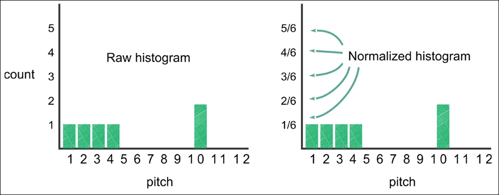
Figure 11: We count the frequency of the loudest pitches heard at each interval to generate this histogram, which acts as our feature vector
Now that we have the chromagram, we need to use it to extract the audio feature to construct a feature vector. You can use the following method for this:
def extract_feature_vector(sess, chromo_data):
    num_features, num_samples = np.shape(chromo_data)
    freq_vals = sess.run(max_freqs, feed_dict={chromo: chromo_data})
    hist, bins = np.histogram(freq_vals, bins=range(num_features +
))
    normalized_hist = hist.astype(float) / num_samples
    return normalized_hist
The workflow of the previous code is as follows:
- Create an operation to identify the pitch with the biggest contribution.
- Now, convert the chromogram into a feature vector.
- After this, we will construct a matrix where each row is a data item.
- Now, if you can hear the audio clip, you can imagine and differentiate between the different audio files. However, this is just intuition.
Therefore, we cannot rely on this, but we should inspect them visually. So, we will invoke the previous method to extract the feature vector from each audio file and plot the feature. The whole operation should look as follows:
def get_dataset(sess):
    num_files = sess.run(count_num_files)
    coord = tf.train.Coordinator()
    threads = tf.train.start_queue_runners(coord=coord)
    xs = list()
    names = list()
    plt.figure()
    for _ in range(num_files):
        chromo_data, filename = get_next_chromogram(sess)
        plt.subplot(1, 2, 1)
        plt.imshow(chromo_data, cmap='Greys', interpolation='nearest')
        plt.title('Visualization of Sound Spectrum')
        plt.subplot(1, 2, 2)
        freq_vals = sess.run(max_freqs, feed_dict={chromo: chromo_data})
        plt.hist(freq_vals)
        plt.title('Histogram of Notes')
        plt.xlabel('Musical Note')
        plt.ylabel('Count')
        plt.savefig('{}.png'.format(filename))
        plt.clf()
        plt.clf()
        names.append(filename)
        x = extract_feature_vector(sess, chromo_data)
        xs.append(x)
    xs = np.asmatrix(xs)
    return xs, names
The previous code should plot the audio features of each audio file in the histogram as follows:

Figure 12: The ride audio files show a similar histogram
You can see some examples of audio files that we are trying to cluster based on their audio features. As you can see, the two on the right appear to have similar histograms. The two on the left also have similar sound spectrums:

Figure 13: The crash cymbal audio files show a similar histogram
Now, the target is to develop K-means so that it is able to group these sounds together accurately. We will look at the high-level view of the cough audio files, as shown in the following figure:

Figure 14: The cough audio files show a similar histogram
Finally, we have the scream audio files that have a similar histogram and audio spectrum, but of course are different compared to others:
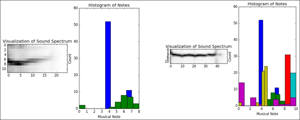
Figure 15: The scream audio files show a similar histogram and audio spectrum
Now, we can imagine our problem. We have the features ready for training the K-means model. Let's start doing it.
- Training K-means model.
Now that the feature vector is ready, it's time to feed this to the K-means model for clustering the feature presented in figure 10. The idea is that the midpoint of all the points in a cluster is called a centroid.
Depending on the audio features we choose to extract, a centroid can capture concepts such as loud sound, high-pitched sound, or saxophone-like sound. Therefore, it's important to note that the K-means algorithm assigns non-descript labels, such as cluster 1, cluster 2, or cluster 3. First, we can write a method that computes the initial cluster centroids as follows:
def initial_cluster_centroids(X, k):
    return X[0:k, :]
Now, the next task is to randomly assign the cluster number to each data point based on the initial cluster assignment. This time we can use another method:
def assign_cluster(X, centroids):
    expanded_vectors = tf.expand_dims(X, 0)
    expanded_centroids = tf.expand_dims(centroids, 1)
    distances = tf.reduce_sum(tf.square(tf.subtract(expanded_vectors, expanded_centroids)), 2)
    calc_wss = tf.reduce_sum(tf.reduce_min(distances, 0))
    mins = tf.argmin(distances, 0)
    return mins, calc_wss
The previous method computes the minimum distance and WCSS for the clustering evaluation in the later steps. Then, we need to update the centroid to check and make sure if there are any changes that occur in the cluster assignment:
def recompute_centroids(X, Y):
    sums = tf.unsorted_segment_sum(X, Y, k)
    counts = tf.unsorted_segment_sum(tf.ones_like(X), Y, k)
    return sums / counts
Now that we have defined many variables, it's time to initialize them using
local_variable_initializer(), as follows:init_op = tf.local_variables_initializer()
Finally, we can perform the training. Forthis, the
audioClusterin()method takes the number of tentative clusters k and iterates the training up to the maximum iteration, as follows:def audioClustering(k, max_iterations ): with tf.Session() as sess: sess.run(init_op) X, names = get_dataset(sess) centroids = initial_cluster_centroids(X, k) i, converged = 0, False while not converged and i < max_iterations: i += 1. Y, wcss_updated = assign_cluster(X, centroids) centroids = sess.run(recompute_centroids(X, Y)) wcss = wcss_updated.eval() print(zip(sess.run(Y)), names) return wcssThe previous method returns the cluster cost, WCSS, and also prints the cluster number against each audio file. So, we have been able to finish the training step. Now, the next task is to evaluate the K-means clustering quality.
- Evaluating the model.
Here, we will evaluate the clustering quality from two perspectives. First, we will observe the predicted cluster number. Secondly, we will also try to find the optimal value of
kas a function of WCSS. So, we will iterate the training for K = 2 to say 10 and observe the clustering result. However, first, let's create two empty lists to hold the values ofKand WCSS in each step:wcss_list = [] k_list = []
Now, let's iterate the training using the
forloop as follows:for k in range(2, 9): random.seed(12345) wcss = audioClustering(k, 100) wcss_list.append(wcss) k_list.append(k)This prints the following output:
 ([(0,), (1,), (1,), (0,), (1,), (0,), (0,), (0,), (0,), (0,), (0,)],
['./audio_dataset/scream_1.wav', './audio_dataset/Crash-Cymbal-3.
wav', './audio_dataset/Ride_Cymbal_1.wav', './audio_dataset/Ride_
Cymbal_2.wav', './audio_dataset/Crash-Cymbal-2.wav', './audio_
dataset/Ride_Cymbal_3.wav', './audio_dataset/scream_3.wav', './
audio_dataset/scream_2.wav', './audio_dataset/cough_2.wav', './audio_
dataset/cough_1.wav', './audio_dataset/Crash-Cymbal-1.wav'])

([(0,), (1,), (2,), (2,), (2,), (2,), (2,), (1,), (2,), (2,), (2,)],
['./audio_dataset/Ride_Cymbal_2.wav', './audio_dataset/Crash-
Cymbal-3.wav', './audio_dataset/cough_1.wav', './audio_dataset/Crash-
Cymbal-2.wav', './audio_dataset/scream_2.wav', './audio_dataset/
Ride_Cymbal_3.wav', './audio_dataset/Crash-Cymbal-1.wav', './
udio_
dataset/Ride_Cymbal_1.wav', './audio_dataset/cough_2.wav', './audio_
dataset/scream_1.wav', './audio_dataset/scream_3.wav'])

([(0,), (1,), (2,), (3,), (2,), (2,), (2,), (2,), (2,), (2,), (2,)],
['./audio_dataset/Ride_Cymbal_2.wav', './audio_dataset/Ride_Cymbal_3.
wav', './audio_dataset/cough_1.wav', './audio_dataset/Crash-Cymbal-1.
wav', './audio_dataset/scream_3.wav', './audio_dataset/cough_2.wav',
'./audio_dataset/Crash-Cymbal-2.wav', './audio_dataset/Ride_Cymbal_1.
wav', './audio_dataset/Crash-Cymbal-3.wav', './audio_dataset/
scream_1.wav', './audio_dataset/scream_2.wav'])

([(0,), (1,), (2,), (3,), (4,), (0,), (0,), (4,), (0,), (0,), (0,)],
['./audio_dataset/cough_1.wav', './audio_dataset/scream_1.wav', './
audio_dataset/Crash-Cymbal-1.wav', './audio_dataset/Ride_Cymbal_2.
wav', './audio_dataset/Crash-Cymbal-3.wav', './audio_dataset/
scream_2.wav', './audio_dataset/cough_2.wav', './audio_dataset/
Ride_Cymbal_1.wav', './audio_dataset/Crash-Cymbal-2.wav', './audio_
dataset/Ride_Cymbal_3.wav', './audio_dataset/scream_3.wav'])

([(0,), (1,), (2,), (3,), (4,), (5,), (2,), (2,), (2,), (4,), (2,)],
['./audio_dataset/scream_3.wav', './audio_dataset/Ride_Cymbal_2.wav',
'./audio_dataset/cough_1.wav', './audio_dataset/Crash-Cymbal-2.wav',
'./audio_dataset/Crash-Cymbal-3.wav', './audio_dataset/scream_2.wav',
'./audio_dataset/Crash-Cymbal-1.wav', './audio_dataset/cough_2.wav',
'./audio_dataset/Ride_Cymbal_3.wav', './audio_dataset/Ride_Cymbal_1.
wav', './audio_dataset/scream_1.wav'])

([(0,), (1,), (2,), (3,), (4,), (5,), (6,), (5,), (6,), (5,), (5,)],
['./audio_dataset/cough_2.wav', './audio_dataset/Ride_Cymbal_3.
av',
'./audio_dataset/scream_1.wav', './audio_dataset/Ride_Cymbal_2.wav',
'./audio_dataset/Crash-Cymbal-1.wav', './audio_dataset/cough_1.wav',
'./audio_dataset/scream_2.wav', './audio_dataset/Crash-Cymbal-3.wav',
'./audio_dataset/scream_3.wav', './audio_dataset/Ride_Cymbal_1.wav',
'./audio_dataset/Crash-Cymbal-2.wav'])

([(0,), (1,), (2,), (3,), (4,), (5,), (6,), (7,), (6,), (6,), (1,)],
['./audio_dataset/Crash-Cymbal-1.wav', './audio_dataset/scream_3.
wav', './audio_dataset/Ride_Cymbal_3.wav', './audio_dataset/
Crash-Cymbal-3.wav', './audio_dataset/Crash-Cymbal-2.wav', './
audio_dataset/cough_2.wav', './audio_dataset/cough_1.wav', './audio_
dataset/Ride_Cymbal_1.wav', './audio_dataset/Ride_Cymbal_2.wav', './
audio_dataset/scream_1.wav', './audio_dataset/scream_2.wav'])

([(0,), (1,), (2,), (3,), (4,), (5,), (6,), (7,), (8,), (1,), (7,)],
['./audio_dataset/scream_2.wav', './audio_dataset/Ride_Cymbal_1.wav',
'./audio_dataset/Crash-Cymbal-2.wav', './audio_dataset/Ride_Cymbal_3.
wav', './audio_dataset/Ride_Cymbal_2.wav', './audio_dataset/scream_3.
wav', './audio_dataset/Crash-Cymbal-1.wav', './audio_dataset/cough_1.
wav', './audio_dataset/cough_2.wav', './audio_dataset/Crash-Cymbal-3.
wav', './audio_dataset/scream_1.wav'])
These values signify that each audio file is clustered and the cluster number has been assigned (the first bracket is the cluster number, the contents in the second bracket is the filename). However, it is difficult to judge the accuracy from this output. One naïve approach would be to compare each file with figure 12 to figure 15. Alternatively, let's adopt a better approach that we used in the first example that is the elbow method. For this, I have created a dictionary using two lists that are
k_listandwcss_listcomputed previously, as follows:dict_list = zip(k_list, wcss_list) my_dict = dict(dict_list) print(my_dict)
The previous code produces the following output:
{2: 2.8408628007260428, 3: 2.3755930780867365, 4: 0.9031724736903582,
5: 0.7849431270192495, 6: 0.872767581979385, 7: 0.62019339653673422,
8: 0.70075249251166494, 9: 0.86645706880532057}
From the previous output, you can see a sharp drop in WCSS for k = 4, and this is generated in the third iteration. So, based on this minimum evaluation, we can take a decision about the following clustering assignment:
Ride_Cymbal_1.wav => 2
Ride_Cymbal_2.wav => 0
cough_1.wav => 2
cough_2.wav =>2
Crash-Cymbal-1.wav =>3
Crash-Cymbal-2.wav => 2
scream_1.wav => 2
scream_2.wav => 2
Now that we have seen two complete examples of using K-means, there is another example called kNN. This is typically a supervised ML algorithm. In the next section, we will see how we can train this algorithm in an unsupervised way for a regression task.