
5
Program Correctness and Verification
This being a book on software testing, one may wonder why we need to talk about program correctness. There are several reasons and some of them are as follows:
- The focus of software testing is to run the candidate program on selected input data and check whether the program behaves correctly with respect to its specification. The behavior of the program can be analyzed only if we know what is a correct behavior; hence the study of correctness is an integral part of software testing.
- The study of program correctness leads to analyze candidate programs at arbitrary levels of granularity; in particular, it leads to make assumptions on the behavior of the program at specific stages in its execution and to verify (or disprove) these assumptions; the same assumptions can be checked at run-time during testing, giving us valuable information as we try to diagnose the program or establish its correctness. Hence the skills that we develop as we try to prove program correctness enable us to be better/more effective testers.
- It is common for program testers and program provers to make polite statements about testing and proving being complementary and then to assiduously ignore each other (each other’s methods). But there is more to complementarity than meets the eye. Very often, what makes a testing method or a proving method ineffective is not an intrinsic attribute of the method, but rather the fact that the method is used against the wrong type of specification. Hence it is advantageous, given a complex/compound specification, to decompose it into two broad components—one that lends itself to testing and the other that lends itself to proving—and apply each method against the appropriate specification component. Consider a simple example: imagine that we want to verify a sorting routine, whose specification is Sort(s,s′) = Ord(s′) ∧ Prm(s,s′), where s designates an array of elements with some ordering key, Ord(s′) means that s′ is ordered (according to selected key), and Prm(s,s′) means that s′ is a permutation of s. Testing the sorting routine against specification Prm(s,s′) is at the same time inefficient, complex, and error prone: it is inefficient because it requires that we save the initial array s to check the property Prm(s,s′) at the end; it is complex because checking that two sequences are permutations of each other is difficult, especially if we allow multiple identical elements; it is error-prone because it is complex. But proving that a sorting routine satisfies the condition Prm(s,s′) is very easy: it suffices to ensure that whenever the array is modified, it is modified in the context of a swap of two of its cells, thereby ensuring the preservation of Prm(s,s′) at each step. By contrast, proving that the sort routine achieves the property Ord(s′) may be tedious and error-prone, as it involves a painstaking inductive argument, and may depend on the stepwise update of index variables and on maintaining complex program invariants; however, checking Ord(s′) at run-time can be done efficiently and reliably; it is efficient because it does not require saving a prior state and can be carried out in O(n) steps (n: the size of the array), and it is reliable because its formula is very simple (ensuring that each element of s′ is not greater than the next element). Hence by testing the program against specification Ord(s′) and proving it against Prm(s,s′), we achieve great gains in efficiency, quality, and reliability.
- It is best to view software testing, not as an isolated effort, but rather as an integral part of a broad, multi-pronged policy of quality assurance that deploys each method where it is most effective by virtue of the Law of Diminishing Returns.
- The study of program verification, which we conduct in this chapter, prepares the ground for the next chapter, where we discuss faults and fault removal.
5.1 CORRECTNESS: A DEFINITION
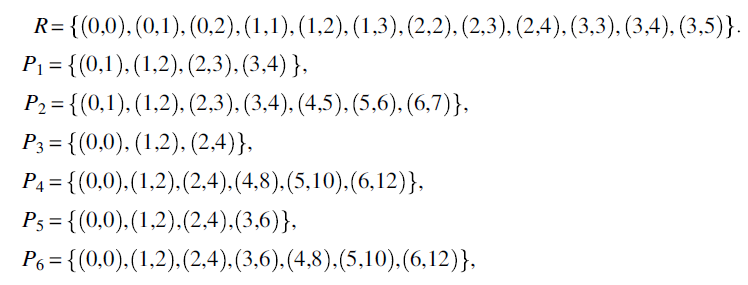
We let space S be the set of natural numbers and let R be the following specification on S:
We consider the following candidate programs (represented by their functions on S), and we ask the question: which of these programs is correct with respect to R?
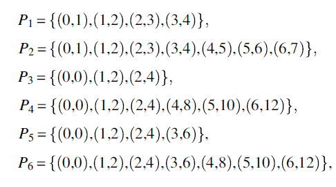
We submit:
- Only programs P1 and P2 are correct with respect to specification R since they return correct values for all the inputs of interest for R (which are inputs 0, 1, 2, 3).
- We say that programs P3 and P4 are partially correct with respect to R: they are not defined for all relevant inputs (which are 0, 1, 2, 3) since they are not defined for 3; but whenever they are defined for a relevant input (which is the case for 0, 1, 2), they return a correct value.
- We say that programs P5 and P6 are defined with respect to R (or that they terminate normally with respect to R): they produce an output for all relevant inputs (which are 0, 1, 2, 3), though for 3 they produce an incorrect output (6, rather than 3, 4, or 5).
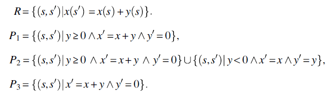
As a second example, we let space S be defined by two integer variables x and y, and we let R be the following relation (specification) on S:
We consider the following candidate programs (written in C-like notation), and we ask the question: which of these programs is correct with respect to R?
p1: {while (y<>0) {x=x+1; y=y-1;}}.p2: {while (y>0) {x=x+1; y=y-1;}}p3: {if (y>0) {while (y>0) {x=x+1; y=y-1;}else {while (y<0) {x=x-1; y=y+1;}}
Before we make judgments on the correctness of these programs, we compute their respective functions:
We submit:
- That P1 is partially correct with respect to R; it is not (totally) correct because it is not defined for negative values of y; but it is partially correct with respect to R because whenever it is defined (for nonnegative values of y), it satisfies specification R (computing the sum of x and y into x).
- That P2 is defined with respect to R; it is not totally correct because for negative y it fails to compute the sum of x and y into x; but it is defined because it produces a final state for all relevant initial states (which, in the case of R, are all states in S).
- That P3 is totally correct with respect to R because it is defined for all relevant initial states and satisfies specification R for all relevant states, by computing the sum of x and y into x.
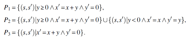
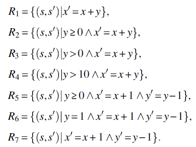
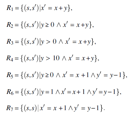
As a third example, we consider the following program on space S defined by integer variables x and y:
p: {while (y<>0) {x=x+1; y=y-1;};}
and we consider the following specifications:
As a reminder, consider that the function of program p is:
Whence we submit:
- Program p is not correct with respect to R1 because it does not terminate for all relevant initial states (which, according to specification R1 are all initial states).
- Program p is correct with respect to specifications R2, R3, R4, and R6. For all these specifications, the program terminates normally for all relevant initial states and delivers a correct final state.
- Program p is defined with respect to specification R5; it is defined for all relevant inputs (which are states such that
 ), but it is not partially correct, since it delivers a different output from what specification R5 demands.
 - Finally, program p is neither correct, nor partially correct, nor defined with respect to specification R7.
We are now ready to cast the intuition gained through these examples into formal definitions.
Note that partial correctness provides for the correct behavior of the program only whenever the program terminates; so that a program that never terminates is, by default, partially correct with respect to any specification. Despite this gaping weakness, partial correctness is a useful property that is often considered valuable in practice.
We conclude this section with a simple proposition, which stems readily from the definitions.
5.2 CORRECTNESS: PROPOSITIONS
In this section, we introduce a number of propositions pertaining to correctness, partial correctness, and termination; for the sake of readability, we do not prove them, but comment on their intuitive significance.
5.2.1 Correctness and Refinement
As we remember, the refinement ordering was introduced in Chapter 4 to rank specifications in terms of strength, reflecting how demanding a specification is or how hard a specification is to satisfy. As we recall, this ordering plays a role in determining whether a given specification is complete with respect to a completeness property and whether a given specification is minimal with respect to a minimality property. Surprisingly, or on second thought not surprisingly, the same refinement ordering plays an important role in defining program correctness, as the following propositions provide. For the sake of simplicity, we restrict our attention to deterministic programs (i.e., programs that produce a uniquely determined final state for any given initial state).
Function P refines relation R if and only if it has a larger domain that R and for all elements s in the domain of R, the pair (s,P(s)) is an element of R; this is exactly how we defined (total) correctness in Section 5.1.
Unlike with total correctness, in partial correctness P does not have to satisfy R for all initial states in the domain of R; rather it suffices that it satisfies R for elements of the domain of R for which p terminates normally (whence the term PL). Note that if we take P=Ø (i.e., program p fails to terminate for all initial states), then this condition is satisfied.
Relation RL has the same domain as relation R, but because it assigns all the elements of S to any element of the domain of R, it imposes no condition on the final state; this is exactly what termination is about.
We conclude this section by revisiting the definition of refinement: so far we have interpreted the refinement to mean that a specification is stronger than another, more demanding than another, and so on. There is a simple way to characterize refinement, now that we have defined correctness; it is given in the following proposition.
Isn’t the essence of being a stronger specification to admit fewer correct programs? Any program that is correct with respect to the stronger/more demanding/more refined specification is necessarily correct with respect to the weaker/less demanding/less refined specification. The necessary condition of this Proposition is a mere consequence of the transitivity of the refinement ordering: if a program p is correct with respect to R, then its function P refines R; since R refines R′, then a fortiori P refines R′, hence p is correct with respect to R′.
5.2.2 Set Theoretic Characterizations
Whereas in Section 5.1 we introduced definitions of correctness and in Section 5.2.1 we introduced propositions that formulate correctness in terms of refinement, in this section we introduce propositions that formulate correctness in terms of set theoretic formulae. In practice, these are more tractable than either the definitions or the refinement-based characterizations.
Interpretation of this formula: The set dom(R) is the set of initial states for which program p must behave as R mandates. The set ![]() is the set of initial states for which program p does behave as R mandates (see Fig. 5.1 for an illustration). Program p is correct with respect to specification R if and only if these two sets are identical.
is the set of initial states for which program p does behave as R mandates (see Fig. 5.1 for an illustration). Program p is correct with respect to specification R if and only if these two sets are identical.
Figure 5.1 Interpretation of dom(R ∩ P).
Interpretation of this formula: The set ![]() is the set of initial states for which program p behaves as R mandates (see Fig. 5.1 for an illustration). The set
is the set of initial states for which program p behaves as R mandates (see Fig. 5.1 for an illustration). The set ![]() is the set of states for which program p terminates and specification R has a requirement. Program p is partially correct with respect to specification R if and only if it behaves according to R whenever it terminates.
is the set of states for which program p terminates and specification R has a requirement. Program p is partially correct with respect to specification R if and only if it behaves according to R whenever it terminates.
This condition simply means that dom(R) is a subset of dom(P).
5.2.3 Illustrations
As an illustration of the propositions given in the previous section, we revisit the examples of Section 5.1 and check the formulas of these propositions to ensure that we reach the same conclusions. We consider the specification and the candidate programs of the first example:
The following table shows, for each candidate program P, the values of ![]() , dom(R), dom(P), and the correctness property of P: total correctness (TC), partial correctness (PC), termination (T), or none (N).
, dom(R), dom(P), and the correctness property of P: total correctness (TC), partial correctness (PC), termination (T), or none (N).
| Candidate |
|
|
|
TC | PC | T | N |
| P1 | {0,1,2,3} | {0,1,2,3} | {0,1,2,3} | ||||
| P2 | {0,1,2,3} | {0,1,2,3} | {0,1,2,3,4,5,6} | ||||
| P3 | {0,1,2} | {0,1,2,3} | {0,1,2} | ||||
| P4 | {0,1,2} | {0,1,2,3} | {0,1,2,4,5,6} | ||||
| P5 | {0,1,2} | {0,1,2,3} | {0,1,2,3} | ||||
| P6 | {0,1,2} | {0,1,2,3} | {0,1,2,3,4,5,6} | ||||
These are indeed the conclusions we had reached earlier for the first example. For the second example, we list the specification and programs, then we draw the same table.
| Candidate |
|
|
|
TC | PC | T | N |
| P1 |
|
S |
|
||||
| P2 |
|
S | S | ||||
| P3 | S | S | S | ||||
These are indeed the conclusions we had reached earlier for the second example. For the third example, we had a single program and many specifications, which we present below:
p: {while (y<>0) {x=x+1; y=y-1;};}
We remember that the function of program p is ![]() , whence the domain of P is
, whence the domain of P is ![]() ; for each specification R we write, in the table below, the values of
; for each specification R we write, in the table below, the values of ![]() , dom(R), and dom(P), then make a judgment about the correctness properties of P with respect to the specification in question.
, dom(R), and dom(P), then make a judgment about the correctness properties of P with respect to the specification in question.
| Specification |
|
|
|
TC | PC | T | N |
| R1 |
|
S |
|
||||
| R2 |
|
|
|
||||
| R3 |
|
|
|
||||
| R4 |
|
|
|
||||
| R5 |
|
|
|
||||
| R6 |
|
|
|
||||
| R7 |
|
S |
|
||||
5.3 VERIFICATION
All the formulas of correctness we have seen so far have an important attribute in common: They define correctness by an equation that involves the function of the candidate program as well as the specification that the program is judged against. In order to use any of these formulas, we need to begin by computing the function of the program. This approach raises two problems: First, computing the function of a program is very complex and error-prone and does not lend itself to automation because it depends (to capture the function of iterative loops) on inductive arguments that are virtually impossible to codify; second, computing the function of a program in all its detail may be wasteful if the specification refers to only partial functional attributes of the program.
For the sake of illustration, consider the following program p on natural variables n, f, k:
{natural n, f, k;f=1; k=1; while (k!=n+1) {f=f*k; k=k+1;}}
and consider the following specifications
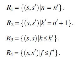
According to the foregoing definitions and propositions, in order to prove that program p is correct with respect to any of the proposed specifications, we must first compute the function of p. Given that the specifications refer to very partial aspects of the function of the program, it seems very wasteful to have to compute the function of the program in all its minute detail before we can prove correctness.
In this section, we present an alternative verification method that is commensurate with the complexity of the specification, and proceeds by recursive descent on the control structure of the program at hand. The core formula of this method takes the form of a triplet:
Where p is a program or program part and φ and ψ are assertions on (variables of) the space of the program. This formula is interpreted as follows: If φ holds prior to execution of program p and p executes and terminates, then ψ holds after the execution of p. Such formulas are called Hoare formulas; φ is called a precondition and ψ is called a postcondition to program p.
5.3.1 Sample Formulas
As a way to nurture the reader’s understanding of this notation, we give below a number of formulas, which we want to consider as valid (in reference to the definition above); we let x and y be integer variables and we classify the sample formulas by the control structure of the program p.
Assignment statement:
- {x=1} x=x+1; {x=2}
- {x≥1} x=x+1; {x≥2}
- {x≥1} x=x+1; {x≥1}
- {x=1 ∧ y=4} x=x+1; {x=2 ∧ y=4}
- {x=x0} x=x+1 {x=x0+1}, for some constant x0.
- {x=x0 ∧ y=y0} x=x+1 {x=x0+1 ∧ y=y0}, for some constants x0 and y0.
- {x=x0 ∧ y=y0} x=x+1 {x≥x0+1 ∧ y≥y0}, for some constants x0 and y0.
Sequence statement:
- {x=3} x=x+3; y=x*x; {x=6 ∧ y=36}
- {x=3} x=x*x; y=x+9 {x=9 ∧ y=18}
- {x=x0 ∧ y=y0} x=x+3; y=x*x; {x=x0+3 ∧ y=(x0+3)2}, for some constants x0 and y0.
- {x=x0 ∧ y=y0} x=x*x; y=x+9; {x=x02 ∧ y=x02+9}, for some constants x0 and y0.
- {x=x0 ∧ y=y0} x=x+y; y=x–y; x=x–y; {x=y0 ∧ y=x0}, for some constants x0 and y0.
- {x=x0 ∧ y=y0} x=x+1; y=y–1; {x=x0+1 ∧ y=y0–1}, for some constants x0 and y0.
- {x=x0 ∧ y=y0} x=x+1; y=y–1; {x+y=x0+y0}, for some constants x0 and y0.
- {x+y=A} x=x+1; y=y–1; {x+y=A}, for some constant A.
Conditional statement:
- {true} if (x<0) {x=−x;} {x≥0}.
- {x=x0} if (x<0) {x=–x;} {x=|x0|}.
- {true} if (x<y) {x=x+y; y=x−y; x=x−y;} {x≥y}.
- {x=x0 ∧ y=y0} if (x<y) {x=x+y; y=x–y; x=x–y;} {x=max(x0,y0) ∧ y=min(x0,y0)}, for some constants x0 and y0.
Alternation statement:
- {x=x0 ∧ y=y0 ∧ x>0 ∧ y>0 ∧ x≠y} if (x>y) {x=x–y ;} else {y=y–x ;} {gcd(x,y)=gcd(x0,y0)}, for some constants x0 and y0.
- {gcd(x,y)=A ∧ x>0 ∧ y>0 ∧ x≠y} if (x>y) {x=x–y ;} else {y=y–x ;} {gcd(x,y)=A}, for some constant A.
Iteration:
- {true} while (y≠0) {x=x+1; y=y–1;} {y=0}
- {y≥0} while (y≠0) {x=x+1; y=y–1;} {y=0}
- {y<0} while (y≠0) {x=x+1; y=y–1;} {y=0}
- {x=x0 ∧ y=y0} while (y≠0) {x=x+1; y=y–1;} {x=x0+y0 ∧ y=0}, for some constants x0 and y0.
- {y≥0} while (y>0) {x=x+1; y=y–1;} {y=0}
- {x=x0 ∧ y≥0} while (y>0) {x=x+1; y=y–1;} {x≥x0}
- {y<0} while (y>0) {x=x+1; y=y–1;} {y<0}
- {x=x0 ∧ y=y0 ∧ y≥0} while (y>0) {x=x+1; y=y–1;} {x=x0+y0 ∧ y=0}, for some constants x0 and y0.
- {x=x0 ∧ y=y0 ∧ y<0} while (y>0) {x=x+1; y=y–1;} {x=x0 ∧ y= y0 ∧ y<0}, for some constants x0 and y0.
- {y<0} while (y≠0) {x=x+1; y=y–1;} {y=–1}
- {y<0} while (y≠0) {x=x+1; y=y–1;} {y=1}
- {y<0} while (y≠0) {x=x+1; y=y–1;} {y=2}
We leave it to the reader to ponder, by reference to the definition of this notation, why each one of the formulas above is valid. So far we have established the validity of these formulas by inspection, in reference to the definition. For larger and more complex programs, this may not be practical; in the next section, we introduce a deductive process that aims to establish the validity of complex formulas by induction on the complexity of the program structure.
5.3.2 An Inference System
An inference system is a system for inferring conclusions from hypotheses in a systematic manner. Such a system can be defined by means of the following artifacts:
- A set F of (syntactically defined) formulas.
- A subset A of F, called the set of axioms, which includes formulas that we assume to be valid by hypothesis.
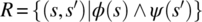
- A set of inference rules, which we denote by R, where each rule is made up of a set of formulas called the premises of the rule, and a formula called the conclusion of the rule. We interpret a rule to mean that whenever the premises of a rule are valid, so is its conclusion; we usually represent a rule by listing its premises above a line and its conclusion below the line.
An inference in an inference system is an ordered sequence of formulas, say v1, v2, …, vn, such each formula in the sequence, say vi, is either an axiom or the conclusion of a rule whose premises appear prior to vi, that is, amongst ![]() . A theorem of a deductive system is any formula that appears in an inference.
. A theorem of a deductive system is any formula that appears in an inference.
In this section, we propose an inference system that enables us to establish the validity of Hoare formulas by induction on the complexity of the program component of the formulas. To this effect, we present in turn, the formulas, then the axioms, and finally the rules.
- Formulas. Formulas of our inference system include all the formulas of logic, as well as Hoare formulas.
- Axioms. Axioms of this inference system include all the tautologies of logic, as well as the following formulas:
- {false} p {ψ}, for any program p and any postcondition ψ.
- {φ} p {true}, for any program p and any precondition φ.
- Rules. We present below a rule for each statement of a simple C-like programming language.
Assignment Statement Rule: We consider an assignment statement that affects a program variable (and implicitly preserving all other variables), and we interpret it as an assignment to the whole program state (changing the selected variable and preserving the other variables), which we denote by s=E(s), where s is the state of the program. We submit the following rule,
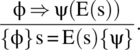
Interpretation: If we want ψ to hold after execution of the assignment statement, when s is replaced by E(s), then ψ(E(s)) must hold before execution of the assignment; hence the precondition φ must imply ψ(E(s)).
Sequence Rule: Let p be a sequence of two subprograms, say p1 and p2. We have the following rule,
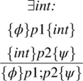
Interpretation: if we can find an intermediate predicate int that serves as a postcondition to p1 and a precondition to p2, then the conclusion is established.
Conditional Rule: Let p be a conditional statement of the form:
if (condition) {statement;}. We have the following rule,
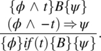
Interpretation: The two premises of this rule correspond to the two execution paths through the flowchart of the conditional statement (Fig. 5.2).
Figure 5.2 Flowchart of if-statement.
Alternation Rule: Let p be an alternation statement of the form:
if (condition) {statement;} else {statement;}. We have the following rule,
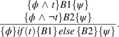
Interpretation: The two premises of this rule correspond to the two execution paths through the flowchart of the conditional statement (Fig. 5.3).
Figure 5.3 Flowchart of if-else statement.
Iteration Rule: Let p be an iterative statement of the form:
while (condition) {statement;}. We have the following rule,
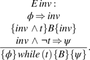
Interpretation: The first and second premises establish an inductive proof to the effect that predicate inv holds after any number of iterations. The third premise provides that upon termination of the loop, the combination of predicate inv and the negation of the loop condition must logically imply the postcondition. Predicate inv is called an invariant assertion. It must be chosen so as to be sufficiently weak to satisfy the first premise, yet sufficient strong to satisfy the third premise (and the second). See the flowchart below, which highlight the points at which each of the relevant assertions is supposed to hold. Note that inv is placed upstream of the loop condition; hence the loop condition is never part of inv (since upstream of the loop condition we do not know whether t is true or not) (Fig. 5.4).
Figure 5.4 Flowchart of while statement.
Consequence Rule: Given a Hoare formula, we can always strengthen the precondition and/or weaken the postcondition. We have the following rule:
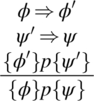
Interpretation: This rule stems readily from the definition of these formulas.
Using the proposed axioms and rules, we can now generate theorems of the form {φ} p {ψ}. The question that arises then is: what good does it do us to generate such theorems? What does that tell us about p? The following Proposition provides the answer.
In the following section, we present sample illustrative examples of the inference system presented herein.
5.3.3 Illustrative Examples
We consider the following program on space S defined by variables x and y of type real, and we form a triplet by embedding it between a precondition and a postcondition:
- Program: while (y≠0) {x=x+1; y=y–1;}.
- Precondition:
 , for some constants x0 and y0.
 - Postcondition:
 .
.
We form the following formula and we attempt to prove that this formula is a theorem of the proposed inference system:
![]()
While (y≠0){x=x+1;y=y−1;} ![]()
We apply the iteration rule to v, using the invariant assertion ![]() . This yields the following three formulas:
. This yields the following three formulas:
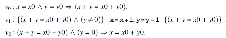
We find that v0 and v2 are both tautologies and hence they are axioms of the inference system. We consider v1, to which we apply the sequence rule, with the intermediate assertion ![]() . This yields two formulas:
. This yields two formulas:
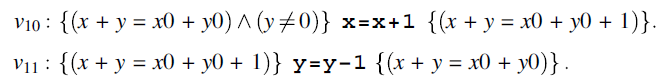
We apply the assignment statement rule to v10 and v11, which yields the following formulas:
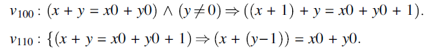
We find that v100 and v110 are both tautologies and hence they are axioms of the inference system. This concludes our proof to the effect that v is a theorem, since the sequence
is an inference, as the reader may check: each formula in this sequence is either an axiom or the conclusion of a rule whose premises are to the left of the formula. By virtue of the proposition labeled Proving Partial Correctness, we conclude that program p is partially correct with respect to the following specification:
It may be more expressive to view this inference as a tree structure, where leaves are the axioms and internal nodes represent the rules that were invoked in the inference; the root of the tree represents the theorem that is established in the inference (Fig. 5.5).
Figure 5.5 Structure of an Inference.
As a second illustrative example, we let space S be defined by three integer variables n, f, k, such that n is nonnegative, and we let program p be defined as:
{f=1; k=1; while (k≠n+1) {f=f*k; k=k+1;};}.
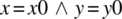
We choose the following precondition and postcondition:
This produces the following formula:
v : {(n = n0)} f=1; k=1; while (k≠n+1) {f=f*k; k=k+1;} {f = n0!}.
We apply the sequence rule to v, using the intermediate predicate ![]() . This yields
. This yields
![]()
![]()
while (k≠n+1) {f=f*k; k=k+1;} {f = n0!}.
We apply the sequence rule to v0, using the intermediate assertion ![]() . This yields
. This yields
![]()
![]()
We apply the assignment statement rule to v00 and v01. This yields respectively:
![]()
![]()
We find that v000 and v010 are both tautologies and hence axioms of the inference system. We now focus on v1, to which we apply the iteration rule, with the invariant assertion ![]() . This yields:
. This yields:
![]()
![]()
![]()
We find that formula v10 is a tautology, since the factorial of 0 is 1, and we find that formula v12 is a tautology, by simple substitution. Hence we now focus on v11, to which we apply the sequence rule, with the intermediate assertion ![]() . This yields:
. This yields:
![]()
![]()
Application of the assignment statement rule to v110 and v111 yields:
![]()
![]()
We find that v1100 and v1110 are both tautologies and hence axioms of the inference system. This concludes our proof; we leave it to the reader to verify that the following sequence is an inference in the proposed inference system:
Because v is a theorem, we conclude that program p is partially correct with respect to the following specification (formed from the precondition and postcondition of v):
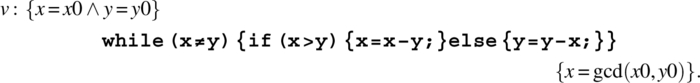
As a third example, we consider the following GCD program on positive integer variables x and y:
{while (x≠y) {if (x>y) {x=x–y;} else {y=y–x;};},
and we consider the following precondition/postcondition pair:
We form the following formula:
We apply the iteration rule to v with the following invariant assertion: ![]() . This yields:
. This yields:
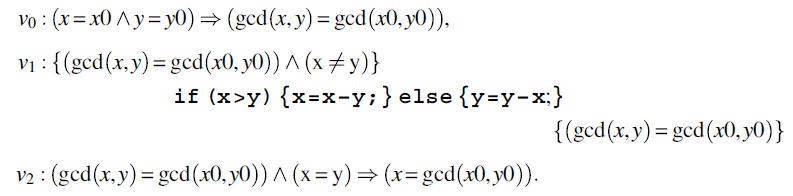
We find that v0 and v2 are tautologies and hence axioms of the inference system. We focus on v1, to which we apply the alternation rule, which yields:
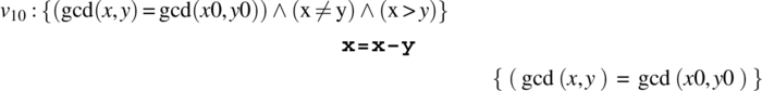
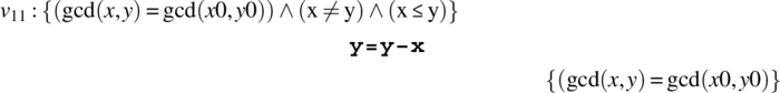
We apply the assignment statement rule to v10 and v11, which yields:
![]()
![]()
We find that both of these formulas are tautologies and hence axioms of the inference system. This concludes the proof that v is a theorem; hence program p is partially correct with respect to
5.4 CHAPTER SUMMARY
Among the most important lessons to retain from this chapter, we cite:
- Understanding that the study of program testing requires that we understand the meaning of program correctness.
- Understanding that a program under test is considered to fail with respect to a specification if it fails to terminate for an initial state in the domain of the specification, or if it does terminate but fails to deliver a state that the specification considers correct.
- Understanding the hierarchy of correctness levels, including total correctness, partial correctness and termination.
- Understanding that all three levels of program correctness can be captured by means of the refinement ordering; in particular, total correctness means precisely that the function of the program refines the specification.
- Understanding the construct of an inference system and how it mechanizes the process of inferring theorems from hypotheses.
- Knowing how to use the proposed inference system to prove that a program is partially correct with respect to a specification that takes the form of a precondition/postcondition.
- Understanding the mapping between a relational specification and a specification that takes the form of a precondition/postcondition.
- Understanding how constants are introduced (and eliminated) from specifications that take the form of a precondition and a postcondition.
5.5 EXERCISES
- 5.1. Prove that the following formula is a theorem of the inference system presented in Section 5.3. Draw a conclusion about the partial correctness of the program.
 .
. - 5.2. Consider the following program on space S defined by variables x, y, z of type integer.
{z=0; while (y≠0) {y=y–1; z=z+x;};}This program computes the product of x and y into z. Write an appropriate precondition and postcondition for this program and prove the resulting formula; compute the binary relation that stems from the precondition/postcondition pair and infer a partial correctness property of the program.
- 5.3. Consider the following program on space S defined by variables n and f of type integer.
{f=1; while (n≠0) {f=f*n; n=n–1;};}Write an appropriate precondition and postcondition that capture the function of this program, and prove the resulting formula; compute the binary relation that stems from the precondition/postcondition pair and infer a partial correctness property of the program.
- 5.4. Same as Exercise 3, for the following program on integer variables x, y, z.
{z=0; while (y≠0) {if (y%2==0) {x=2*x; y=y/2;} else {z=z+x; y=y–1;};};}. - 5.5 Same as Exercise 3, for the following program on real array a of size N (≥1), variable x of type real, and index variable k:
{x=0; k=0; while (k<N) {x=x+a[k]; k=k+1;};}. - 5.6 Same as Exercise 3, for the following program on real array a of size N (≥1), variable x of type real, variable f of type Boolean, and index variable k:
{k=N–1; a[0]=x; while (a[k]≠x) {k=k–1;}; f=(k>0);} - 5.7 Draw the inference tree of the proof of the second example (the factorial program) in Section 5.3.3.
- 5.8 Draw the inference tree of the proof of the third example (the gcd program) in Section 5.3.3.
5.6 PROBLEMS
- 5.1. Imagine that we have a program p on space S and a specification R on S, and we wish to prove that p is partially correct with respect to R using the inference system of Section 5.3. How we do convert specification R into a precondition and a postcondition? Is this conversion unique? Give illustrative examples.
- 5.2. When we are given a precondition φ and a postcondition ψ of a program p, we can use them to form a relational specification R by the formula
 . When constants (such as x0 and y0) are involved in the precondition or postcondition, we must quantify them existentially in the formula of R; justify this step. Give an example of a precondition/postcondition pair that adequately describes the function of a program but can be defined without reference to constants.
5.7 BIBLIOGRAPHIC NOTES
The definitions and propositions pertaining to program correctness are due to Linger et al. (1979) and Mills et al. (1986) or inspired from Mili et al. (1994). The proof method that is presented in Section 5.3.2 is due to C.A.R. Hoare (1969).