3
Self‐Sustaining Wireless Neighborhood‐Area Network Design
Wireless technology has been widely considered for last‐mile communications in the smart grid, because of its growing performance and the relatively low cost but more flexible nature. In the advanced metering infrastructure (AMI), both home‐area networks (HANs) and neighborhood‐area networks (NANs) can be deployed using wireless technologies. While HAN has been widely studied using either IEEE 802.11 (Wi‐Fi) or IEEE 802.15.4 (ZigBee) due to its small coverage and low data rate transmission [53, 54], the standalone NAN should be explored. In this chapter, we propose a self‐sustaining wireless NAN design for AMI in the smart grid. We then propose an optimization approach to achieve minimum total cost for the design. To optimize the system, we first study the optimal number of gateway DAPs. Then we propose two geographical deployment methods in order to achieve fairness for customers. To further enhance fairness, we set different transmission power levels for gateway DAPs. We also achieve the global uplink transmission power efficiency. Compared with the existing game theoretical approach, our approach can increase the energy efficiency of the system. To quickly approach the optimal result, we propose an algorithm for which the computational complexity depends solely on solving a linear system.
3.1 Overview of the Proposed NAN
3.1.1 Background and Motivation of a Self‐Sustaining Wireless NAN
In a neighborhood powered by the smart grid, each household or apartment (we will use only household hereafter since the DAPs are not affected by the types of customers) is equipped with a smart meter. Besides residential customers, commercial and industrial customers are also equipped with smart meters in their buildings and parking lots with electric vehicle charging ports. Each smart meter collects facility status and customer‐side power usage. Smart meters are connected to the service provider through the NAN and WAN to upload customer information to the service provider. The service provider sends real time pricing and tariff information to all the smart meters through downlinks.
A NAN consists of multiple DAPs. Each DAP collects data from a group of nearby smart meters. Unlike a HAN, which is deployed in a protected household, a NAN is most likely to be deployed in an open public area; it must be low‐profile and flexible so it can be easily deployed, moved, or replaced. Unlike a WAN, which is powered by the grid directly and has a wired connection to satisfy its Gbps‐level data rate, a wireless‐based NAN has a much lower data transmission rate. Fortunately, a NAN does not require a Gbps‐level data rate. In practice, a smart meter generates about 12 KBytes of data during one sampling period [34]. In that case, short‐range wireless technology such as Wi‐Fi would provide sufficient performance for local transmission within a NAN [58]. Moreover, operating a wireless‐based NAN does not require too much power, which makes it possible to apply renewable energy (e.g. solar power) to the NAN design.
However, Wi‐Fi is not a good solution to longer distances (e.g. uplink/downlink transmission of NAN gateways to/from the concentrator). A solution is to use cellular communication technologies, for instance IEEE 802.16 (WiMAX) [59], for NAN gateways. Note that the term gateway is used interchangeably with NAN gateway in the rest of the chapter. Ideally, WiMAX provides a data rate up to 70 Mbps and distance up to 48 kilometers [60]. Although those two cannot be achieved at the same time, a high data rate can be achieved when the distance is relatively short in a neighborhood. WiMAX also has an advantage over other types of longer distance wireless transmission (e.g. LTE) in that it can be operated in an unlicensed spectrum under FCC rules [61].
Since a larger number of hops in a mesh network results in a longer delay [62], some gateways need to be deployed in the NAN. In addition to reducing end‐to‐end delay, multiple gateways would also enhance the reliability of the NAN [63]. However, a larger number of gateways does not necessarily produce better transmission performance. It is important to find the optimal number of gateways in a NAN. In this design, we will focus on the scenario with a single concentrator.
3.1.2 Structure of the Proposed NAN
The proposed self‐sustaining wireless NAN design is based on an IEEE 802.11s-enabled (or Wi-Fi based) [64] wireless mesh structure. An overview of the NAN design is shown in Figure 3.1. The NAN consists of a concentrator and a number of DAPs. The concentrator is deployed close to the neighborhood. It is connected to the wired backhaul network for communicating with the service provider. DAPs are deployed to cover the entire neighborhood. Each of them collects data from several surrounding smart meters and uploads the data to the concentrator. Each DAP also broadcasts controlling information from the service provider to those smart meters.

Figure 3.1 Overview of the proposed NAN structure.
IEEE 802.15.4 (ZigBee) has been widely adopted for HANs and thus is assumed to be the technology used for communications within a HAN and between a HAN and a DAP [64]. Unlike the single‐hop low data rate transmissions between a HAN and a DAP, local NAN transmissions among DAPs introduce multihop wireless mesh networking. Therefore it requires a higher data rate for the transmissions. IEEE 802.11s (Wi‐Fi‐based wireless mesh network) is a good candidate, since it meets these criteria. Among all the DAPs, some of them are chosen as the gateway DAPs which communicate with the concentrator directly. Although Wi‐Fi performs well in local NAN transmission, its transmission range is limited; therefore it can hardly support uplink and downlink transmission between gateway DAPs and the concentrator at longer distances (i.e. hundreds of meters). As a solution for gateway DAPs, we adopt IEEE 802.16 (WiMAX) as the technology for transmission. Using WiMAX has an extra benefit compared with similar technologies (e.g. UMTS or LTE). WiMAX can be deployed using an unlicensed band (e.g. ![]() ) in order to lower the service cost by avoiding license fees for band access. However, the use of unlicensed bandwidth must follow certain restrictions imposed by the FCC [61].
) in order to lower the service cost by avoiding license fees for band access. However, the use of unlicensed bandwidth must follow certain restrictions imposed by the FCC [61].
Normal DAPs are deployed in the neighborhood to cover all customers. The number and the geographical positions of gateway DAPs must be carefully chosen so that the data from all the customers can reach the concentrator in time. Traditionally, a network may only have one or multiple gateways that are located closer to the destination compared with other units within this network. However, multiple gateways need to be deployed sparsely in a NAN because of its wide‐ranging latency requirement (3 ms to 5 min) [65, 66]. If some metering data has too many hops to reach a gateway, it may not get delivered within the latency requirement.
To achieve self‐sustainability, the DAPs are powered by renewable energy (e.g. solar power). Compared with the design powered by a power line, using renewable energy will significantly reduce the construction cost, since the location for deploying a DAP does not need physical access to a power outlet. The flexibility and lower cost also ease the burden of maintenance and system upgrades (e.g. replacement or relocation of the DAPs) in the future. Moreover, a system that must be plugged into an outlet will be useless during emergency situations such as an outage. However, during such blackouts it is critical for the service provider to get power line status or to send out control messages. Therefore, being independent of the traditional power supply is an advantage of the proposed wireless NAN design.
3.2 Preliminaries
In this section, some preliminaries are presented so that design details of the proposed NAN can be better described. We assume each DAP is powered by solar power and a backup battery with limited capacity. Thus we will show the modeling of solar panel charging and battery life cycle. We will also mention the path loss model used for wireless transmissions in the NAN design.
3.2.1 Charging Rate Estimate
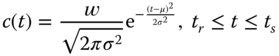
The charging rate estimate is modeled for a solar panel that powers a DAP. For simplicity, we assume that the maximum charging rate occurs at noon (assuming 12:00 p.m.) and the minimum charging rate occurs at sunrise and sunset. Moreover, let the charging rate be symmetric during the daytime. Then the charging rate at time ![]() with perfect weather conditions is estimated as follows:
with perfect weather conditions is estimated as follows:
where ![]() ,
, ![]() is the parameter that determines the
is the parameter that determines the ![]() (e.g. noon/sunrise) charging ratio,
(e.g. noon/sunrise) charging ratio, ![]() is the weight factor depending on number of the solar panels and weather conditions, and
is the weight factor depending on number of the solar panels and weather conditions, and ![]() are sunrise time and sunset time respectively. In other words,
are sunrise time and sunset time respectively. In other words, ![]() is a value determined by the nature of the solar panel, and
is a value determined by the nature of the solar panel, and ![]() is determined by the size of solar panel.
is determined by the size of solar panel.
For example, as stated in [67], the ![]() charging ratio with sunny weather conditions is about 2.94. Even with cloudy weather conditions, the solar panel can still generate electricity with a
charging ratio with sunny weather conditions is about 2.94. Even with cloudy weather conditions, the solar panel can still generate electricity with a ![]() charging ratio of about 2.33. With these facts, we find
charging ratio of about 2.33. With these facts, we find ![]() and
and ![]() for sunny and cloudy weather conditions respectively. Although a solar panel still functions with imperfect weather conditions, it generates electricity at a significantly lower rate. The ratio of the maximum charging rate during sunny weather to that of cloudy weather is about 6.71. Equivalently speaking, we have
for sunny and cloudy weather conditions respectively. Although a solar panel still functions with imperfect weather conditions, it generates electricity at a significantly lower rate. The ratio of the maximum charging rate during sunny weather to that of cloudy weather is about 6.71. Equivalently speaking, we have ![]() . If a unit solar panel has a maximum charging rate of 1 W during sunny weather, then its
. If a unit solar panel has a maximum charging rate of 1 W during sunny weather, then its ![]() and
and ![]() . The charging characteristics during perfect weather conditions of such a solar panel unit are shown in Figure 3.2. Without loss of generality, cloudy weather is applied to illustrate all bad weather, such as rainy or foggy conditions.
. The charging characteristics during perfect weather conditions of such a solar panel unit are shown in Figure 3.2. Without loss of generality, cloudy weather is applied to illustrate all bad weather, such as rainy or foggy conditions.

Figure 3.2 Solar panel charging rate estimate.
Although the performance of a solar panel varies in different seasons, we assume the size needed is determined based on the worst season (normally winter). In the rest of the paper, for simplicity we assume the sunny weather and cloudy weather conditions are those of typical days in winter.
3.2.2 Battery‐Related Issues
The first issue for a battery is the charging cycle. The battery has to be replaced if its state of health (SoH) falls below ![]() of rated capacity [68]. The
of rated capacity [68]. The ![]() is updated after one charge; for simplicity, we adopt the linear estimation as:
is updated after one charge; for simplicity, we adopt the linear estimation as:
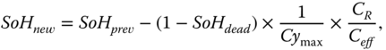
where ![]() is the maximum battery life cycle,
is the maximum battery life cycle, ![]() is the rated capacity, and
is the rated capacity, and ![]() is the effective capacity highly effected by discharging current
is the effective capacity highly effected by discharging current ![]() for discharging time
for discharging time ![]() (typically 20 hours), where
(typically 20 hours), where

However, the discharging current for a DAP is relatively small (![]() ), and thus
), and thus ![]() . In the following discussion, the effective capacity is thus omitted. To make the illustration clearer, let the deterioration of health (
. In the following discussion, the effective capacity is thus omitted. To make the illustration clearer, let the deterioration of health (![]() ) be the status of the battery to monitor. And thus
) be the status of the battery to monitor. And thus ![]() accordingly. We rewrite Eq. (3.2) as:
accordingly. We rewrite Eq. (3.2) as:

For simplicity, we assume that the maximum battery life cycles ![]() depends solely on the depth of discharge (DoD); for example, when
depends solely on the depth of discharge (DoD); for example, when ![]() ,
, ![]() .
.

We model the maximum cycles under different ![]() with several linear segments based on data given in Table 3.1 [69]. The estimates are calculated by Eq. (3.5). Figure 3.3 also illustrates the estimates of maximum cycles with different depths of discharge.
with several linear segments based on data given in Table 3.1 [69]. The estimates are calculated by Eq. (3.5). Figure 3.3 also illustrates the estimates of maximum cycles with different depths of discharge.
Table 3.1 Selected DoDs and their maximum cycles.
| Depth of discharge ( | Maximum cycles |
| 100 | 300 |
| 80 | 500 |
| 50 | 1200 |
| 25 | 2000 |
| 10 | 4000 |
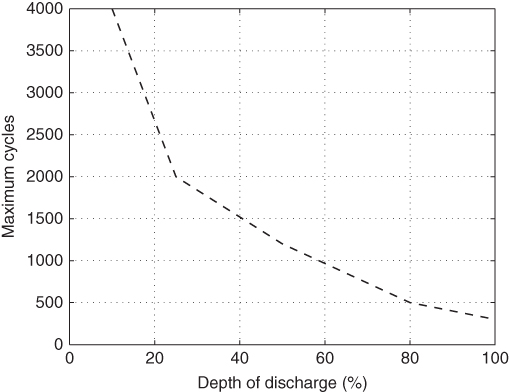
Figure 3.3 Modeling of maximum cycles against depth of discharge.
3.2.3 Path Loss Model
The uplink transmission from a gateway DAP to the concentrator is usually further than a close‐in reference distance (e.g. 100 m), and it is much further than a single‐hop local transmission; therefore we need to apply path loss to the transmission model. Path loss is not considered in Wi‐Fi transmission within the NAN. Wi‐Fi transmission loss has been considered as the receiving data rate being significantly lower than theoretical limit of the physical layer data rate. There are two well‐known path loss models used to estimate the WiMAX path loss in smart grid communication: one is the modified Hata model (also known as the COST 231 model) and the other one is the Erceg model [70].
The modified Hata model is applicable from 1500 MHz to 2000 MHz and with a frequency correction factor ![]() can be extended to higher frequencies. The path loss is calculated as
can be extended to higher frequencies. The path loss is calculated as

where ![]() is the path distance in kilometers,
is the path distance in kilometers, ![]() is the frequency in megahertz,
is the frequency in megahertz, ![]() is the base station (concentrator) antenna height,
is the base station (concentrator) antenna height, ![]() is the subscriber station (DAP) antenna height, and
is the subscriber station (DAP) antenna height, and ![]() is calculated as:
is calculated as:

For urban environments, ![]() = 3 dB and
= 3 dB and
For suburban environments, ![]() = 0 dB, and
= 0 dB, and
The Erceg model is considered applicable from 1800 MHz to 2700 MHz; it also adopts a correction function for higher frequency. The path loss is calculated as:

In addition to the parameters used in the modified Hata model, here ![]() m, and
m, and ![]() is the wavelength in meters. The correction function
is the wavelength in meters. The correction function ![]() [71] for higher frequency is
[71] for higher frequency is
where ![]() MHz and
MHz and ![]() in most settings. The Erceg model has three sets of settings which apply to three terrain types. Type A is hilly with moderate to heavy tree density, type B is hilly with light tree density or flat and moderate to heavy tree density, and type C is flat with light tree density. The detailed settings are shown in Table 3.2.
in most settings. The Erceg model has three sets of settings which apply to three terrain types. Type A is hilly with moderate to heavy tree density, type B is hilly with light tree density or flat and moderate to heavy tree density, and type C is flat with light tree density. The detailed settings are shown in Table 3.2.
Table 3.2 The remaining parameters for the Erceg model.
| Parameter | Type A | Type B | Type C |
| a | 4.6 | 4.0 | 3.6 |
| b | 0.0075 | 0.0065 | 0.005 |
| c | 12.6 | 17.1 | 20 |
| X | 10.8 | 10.8 | 20 |
Suppose that the WiMAX operates at the 5.8 GHz unlicensed band, the path distance ![]() = 2 km, the concentrator antenna height
= 2 km, the concentrator antenna height ![]() = 10 m, and the DAP antenna height
= 10 m, and the DAP antenna height ![]() = 2 m. The modified Hata model in a suburban environment gives
= 2 m. The modified Hata model in a suburban environment gives ![]() . As a comparison, the Erceg model [71] in hilly terrain with light tree density or flat terrain with moderate to heavy tree density gives 139.67 dB. The two models give close results; therefore, we adopt the modified Hata model for simplicity. Applying the maximum transmission power
. As a comparison, the Erceg model [71] in hilly terrain with light tree density or flat terrain with moderate to heavy tree density gives 139.67 dB. The two models give close results; therefore, we adopt the modified Hata model for simplicity. Applying the maximum transmission power ![]() dBm allowed by the FCC, the receiving power is
dBm allowed by the FCC, the receiving power is ![]() dBm respectively, which is higher than the receiving sensitivity (widely accepted as −120 dBm). Apparently, operating at a lower licensed band will lead to lower path loss.
dBm respectively, which is higher than the receiving sensitivity (widely accepted as −120 dBm). Apparently, operating at a lower licensed band will lead to lower path loss.
3.3 Problem Formulations and Solutions in the NAN Design
In this section, we will discuss the core problems of the proposed NAN design. The problems include cost minimization, optimal number of gateways, deployment of gateway DAPs, and global uplink transmission power efficiency. The problems and solutions explored in this section may serve as guidelines and benchmarks for future NAN deployment in the smart grid.
3.3.1 The Cost Minimization Problem
Generally speaking, the ultimate goal in the NAN design is to minimize the total cost for the NAN to operate for a certain number of years, for example, ![]() years. The total cost of a NAN consists of three parts: deployment cost, operational cost, and maintenance cost. Deployment cost includes the cost of all the hardware, including DAPs, gateway DAPs, batteries, solar panels etc. Operation cost includes power usage (which is zero for renewable energy), the data subscription fee if a licensed band is used, etc. And maintenance cost includes the replacement of any malfunctioning equipment, plus labor costs and any monetary loss due to missing data.
years. The total cost of a NAN consists of three parts: deployment cost, operational cost, and maintenance cost. Deployment cost includes the cost of all the hardware, including DAPs, gateway DAPs, batteries, solar panels etc. Operation cost includes power usage (which is zero for renewable energy), the data subscription fee if a licensed band is used, etc. And maintenance cost includes the replacement of any malfunctioning equipment, plus labor costs and any monetary loss due to missing data.
In reality, the NAN is supposed to handle a small amount of data; thus it is safe to assume that a self‐sustaining network without maintenance is more cost efficient. By adopting pure renewable energy and unlicensed bands, the operation cost is excluded as well. Therefore, it is reasonable to assume that the total cost for the NAN depends on the deployment cost only. In our NAN design, the equivalent problem is to find the optimal combination of battery size and solar panel size for each DAP so that the minimum total cost could be achieved. Let ![]() be the price of a unit size battery (e.g. 1 Wh), and
be the price of a unit size battery (e.g. 1 Wh), and ![]() be the price of a unit size solar panel. For the deployment, the objective is to find
be the price of a unit size solar panel. For the deployment, the objective is to find
where ![]() is the battery size,
is the battery size, ![]() is the solar panel size for DAP
is the solar panel size for DAP ![]() , and
, and ![]() is the set of all DAPs. For a DAP
is the set of all DAPs. For a DAP ![]() to sustain the system for
to sustain the system for ![]() years, its battery must last
years, its battery must last ![]() days before reaching the end of its state of health, that is,
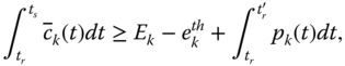
days before reaching the end of its state of health, that is, ![]() . Thus the battery is not supposed to be charged every day according to previous discussions. The battery should be charged only when its remaining energy falls below a threshold
. Thus the battery is not supposed to be charged every day according to previous discussions. The battery should be charged only when its remaining energy falls below a threshold ![]() . This threshold is set based on a critical situation, e.g.
. This threshold is set based on a critical situation, e.g. ![]() continuous cloudy days, as follows:
continuous cloudy days, as follows:

where ![]() is the charging rate for DAP
is the charging rate for DAP ![]() in cloudy weather and
in cloudy weather and ![]() is the power usage at time
is the power usage at time ![]() . Let the original battery capacity of DAP
. Let the original battery capacity of DAP ![]() be
be ![]() . For practical purposes, we also set the charging threshold to be no less than
. For practical purposes, we also set the charging threshold to be no less than ![]() , such that
, such that
Note that ![]() will trigger the charging signal; however, the actual charging may not happen immediately. For example, the threshold may be reached during night time. Assuming that
will trigger the charging signal; however, the actual charging may not happen immediately. For example, the threshold may be reached during night time. Assuming that ![]() is reached at
is reached at ![]() , then at sunrise time
, then at sunrise time ![]() , the remaining battery capacity will be
, the remaining battery capacity will be ![]() . In this case, if the next day is a sunny day, the battery should be fully charged at sunset
. In this case, if the next day is a sunny day, the battery should be fully charged at sunset ![]() on that day. If the battery cannot be fully charged on a sunny day, it will not be fully charged under any circumstances. Because once
on that day. If the battery cannot be fully charged on a sunny day, it will not be fully charged under any circumstances. Because once ![]() , the indicator of charge is off, and the next charge cycle occurs when
, the indicator of charge is off, and the next charge cycle occurs when ![]() . However, the battery will not fully charged again, and the DAP consumes power for the whole day (
. However, the battery will not fully charged again, and the DAP consumes power for the whole day (![]() ).
).
The sunny day charging constraint is set as follows:
where ![]() is the charging rate in a sunny day at time
is the charging rate in a sunny day at time ![]() . Note that the daytime power consumption is merged with the previous nighttime power consumption and is expressed as the whole day power consumption. To make the illustration clearer, we also show in Eq. (3.16) that on a sunny day at sunrise time
. Note that the daytime power consumption is merged with the previous nighttime power consumption and is expressed as the whole day power consumption. To make the illustration clearer, we also show in Eq. (3.16) that on a sunny day at sunrise time ![]() , the charging rate is already above the corresponding power usage, such that
, the charging rate is already above the corresponding power usage, such that
A larger solar panel is able to charge the battery faster; however, waste in resources needs to be avoided. Thus, let the upper bound be set such that the DAP can be self‐sustaining if every day is cloudy throughout ![]() years. Thus the constraint for the solar panel size is shown in Eq. (3.17).
years. Thus the constraint for the solar panel size is shown in Eq. (3.17).

Moreover, the battery must survive the designed life cycle, such that
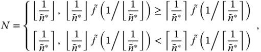
Constraint Eq. (3.18) is further relaxed for simplicity and with the practical purpose of finally solving the optimization problem. We define ![]() as an estimate of the pseudo‐shortest charging period for DAP
as an estimate of the pseudo‐shortest charging period for DAP ![]() . It is estimated based on a fully charged DAP that operates through continuously cloudy days before it reaches the threshold. Thus
. It is estimated based on a fully charged DAP that operates through continuously cloudy days before it reaches the threshold. Thus ![]() is estimated as follows:
is estimated as follows:
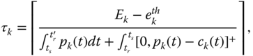
where ![]() returns the larger element of the two. The denominator is the remaining energy before a charging signal is triggered. The numerator is the DAP power consumption in a whole day, which consists of two parts. 1)
returns the larger element of the two. The denominator is the remaining energy before a charging signal is triggered. The numerator is the DAP power consumption in a whole day, which consists of two parts. 1) ![]() is the nighttime power consumption, and 2)
is the nighttime power consumption, and 2) ![]() is the daytime power consumption. Obviously, if
is the daytime power consumption. Obviously, if ![]() , the DAP is powered by its solar panel and does not consume battery energy. Note that
, the DAP is powered by its solar panel and does not consume battery energy. Note that ![]() is not the shortest delay between two charges because a DAP with a partially charged battery that operates through continuous cloudy days may cause a shorter delay between two charges. However, if only extreme cases are considered, the design will end up with unnecessarily large battery and solar panel. The parameter
is not the shortest delay between two charges because a DAP with a partially charged battery that operates through continuous cloudy days may cause a shorter delay between two charges. However, if only extreme cases are considered, the design will end up with unnecessarily large battery and solar panel. The parameter ![]() is validated to be practical in the case study.
is validated to be practical in the case study.
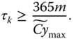
Let ![]() be an estimated maximum charging cycle based on a deep
be an estimated maximum charging cycle based on a deep ![]() (e.g. 500 when
(e.g. 500 when ![]() ). In order to survive the designed life cycle, instead of using constraint Eq. (3.18), we apply the following constraint:
). In order to survive the designed life cycle, instead of using constraint Eq. (3.18), we apply the following constraint:
The DAP needs to record several types of data in two consecutive days (e.g. days ![]() and
and ![]() ) for further evaluation. First, it needs to record a time stamp
) for further evaluation. First, it needs to record a time stamp ![]() when
when ![]() for the first time and also record
for the first time and also record ![]() on each day, (e.g.
on each day, (e.g. ![]() for day
for day ![]() ). The DAP also needs to record a daily charging cycle indicator (e.g.
). The DAP also needs to record a daily charging cycle indicator (e.g. ![]() for day
for day ![]() ). If
). If ![]() , then
, then ![]() , where
, where ![]() is an XOR function. Note that the battery will be charged at most once per day. Another indicator to be recorded is
is an XOR function. Note that the battery will be charged at most once per day. Another indicator to be recorded is ![]() . Based on
. Based on ![]() and
and ![]() ,
, ![]() is calculated as follows:
is calculated as follows:
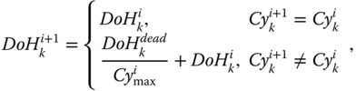
where ![]() is determined by
is determined by ![]() according to Eq. (3.5).
according to Eq. (3.5).
DAPs are independent of each other, as they do not share solar panels or batteries. Therefore, the total cost optimization problem can be approached individually for each DAP if the number of normal DAPs and gateway DAPs are determined (which will be discussed later). Therefore, solving the problem shown in Eq. (3.12) is equivalent to solving the problem as follows:
subject to
Constraints (3.19) and (3.20),
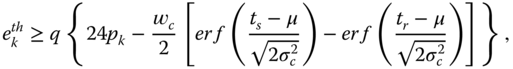
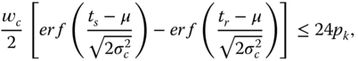
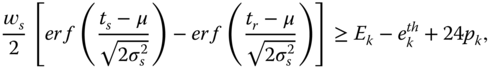

Assume each DAP operates at a constant power consumption (i.e. ![]() ). After applying the charging rate estimation functions, new constraints Eq. (3.23), Eq. (3.24), Eq. (3.25), and Eq. (3.26) are rewritten from Eq. (3.13), Eq. (3.17), Eq. (3.15), and Eq. (3.16) respectively. With any given
). After applying the charging rate estimation functions, new constraints Eq. (3.23), Eq. (3.24), Eq. (3.25), and Eq. (3.26) are rewritten from Eq. (3.13), Eq. (3.17), Eq. (3.15), and Eq. (3.16) respectively. With any given ![]() , Eq. (3.22) is a linear optimization problem that can be solved efficiently. For normal DAPs, which are basically Wi‐Fi routers, their power consumption is constant (e.g.
, Eq. (3.22) is a linear optimization problem that can be solved efficiently. For normal DAPs, which are basically Wi‐Fi routers, their power consumption is constant (e.g. ![]() mW or
mW or ![]() dBm). Therefore, the cost for normal DAPs can be determined so far. However, the power consumption for gateway DAPS ranges from 100 mW to 1 W. The method of deployment and number of gateway DAPs would highly affect the service quality to customers. It is not recommended to arbitrarily assign a power consumption level to a gateway DAP. Therefore, we need to first determine the number
dBm). Therefore, the cost for normal DAPs can be determined so far. However, the power consumption for gateway DAPS ranges from 100 mW to 1 W. The method of deployment and number of gateway DAPs would highly affect the service quality to customers. It is not recommended to arbitrarily assign a power consumption level to a gateway DAP. Therefore, we need to first determine the number ![]() of gateway DAPs and then optimize the uplink transmission power consumption
of gateway DAPs and then optimize the uplink transmission power consumption ![]() for each of them.
for each of them.
3.3.2 Optimal Number of Gateways
In much of the research regarding power control for multiple‐access systems [72–75], the effective transmission rate (or the receiving data rate) for a transmitter (e.g. gateway DAP ![]() ) is expressed as follows:
) is expressed as follows:
where ![]() is the physical layer transmission rate and
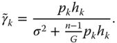
is the physical layer transmission rate and ![]() is the signal‐to‐interference‐plus‐noise (SINR) ratio. The SINR is calculated as follows:
is the signal‐to‐interference‐plus‐noise (SINR) ratio. The SINR is calculated as follows:

where ![]() is the processing gain. In Eq. (3.27),
is the processing gain. In Eq. (3.27), ![]() is the efficiency function that calculates the probability of a packet being successfully transmitted. Function
is the efficiency function that calculates the probability of a packet being successfully transmitted. Function ![]() is widely adopted as an increasing, continuous, and S‐shaped function with
is widely adopted as an increasing, continuous, and S‐shaped function with ![]() ,
, ![]() predetermined. Mathematically, the efficiency function can be as follows:
predetermined. Mathematically, the efficiency function can be as follows:
where ![]() is the packet length.
is the packet length.
Let ![]() be the indicators of gateway DAPs, and
be the indicators of gateway DAPs, and ![]() be the total number of gateway DAPs. We then discuss the optimal
be the total number of gateway DAPs. We then discuss the optimal ![]() needed for a specific NAN. Since usage, coverage, and customer numbers of the smart grid, the optimal number is one that supports a maximum upload transmission data rate in a NAN that provides for future upgrades. This problem is formulated as follows:
needed for a specific NAN. Since usage, coverage, and customer numbers of the smart grid, the optimal number is one that supports a maximum upload transmission data rate in a NAN that provides for future upgrades. This problem is formulated as follows:

where ![]() is the set of positive integers. We assume that each gateway DAP covers the same number of users regardless of its distance to the concentrator. Then the receiving power at the concentrator for each gateway needs to be identical, that is,
is the set of positive integers. We assume that each gateway DAP covers the same number of users regardless of its distance to the concentrator. Then the receiving power at the concentrator for each gateway needs to be identical, that is, ![]() , so that all smart meters will be treated fairly independent of their distance to the gateway. Since
, so that all smart meters will be treated fairly independent of their distance to the gateway. Since ![]() shall be a constant for later discussion, we replace it with a variable
shall be a constant for later discussion, we replace it with a variable ![]() for solving Eq. (3.30) in this subsection. Eq. (3.28) is then rewritten as follows:
for solving Eq. (3.30) in this subsection. Eq. (3.28) is then rewritten as follows:
For simplicity, path gain is represented as follows:
where ![]() is the distance between the gateway
is the distance between the gateway ![]() and the concentrator and
and the concentrator and ![]() is the fading parameter. Thus the receiving power can be written as
is the fading parameter. Thus the receiving power can be written as
Obviously, ![]() increases with respect to
increases with respect to ![]() ,
, ![]() . The maximum SINR
. The maximum SINR ![]() is achieved when
is achieved when ![]() . Note that
. Note that ![]() depends on the furthest gateway, since it has the lowest path gain. Thus the maximum SINR is calculated as follows:
depends on the furthest gateway, since it has the lowest path gain. Thus the maximum SINR is calculated as follows:
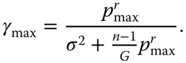
Note that the noise ![]() (e.g. −120 dBm) is not negligible compared with
(e.g. −120 dBm) is not negligible compared with ![]() (e.g., −110 dBm). With a given
(e.g., −110 dBm). With a given ![]() , the efficiency function is a function with respect to
, the efficiency function is a function with respect to ![]() (note that
(note that ![]() is a positive integer) such that
is a positive integer) such that
The estimated maximum total transmission data rate from all the gateways ![]() is calculated as follows:
is calculated as follows:

With that, the objective in Eq. (3.30) can be presented equivalently as follows:
Let ![]() , then
, then ![]() can be calculated equally as follows:
can be calculated equally as follows:

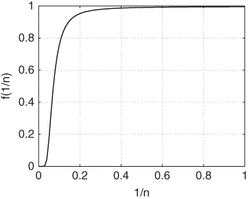
Figure 3.4 ‐function
  .
.
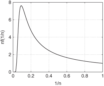
Figure 3.5 A quasiconcave function.
Now that we know Eq. (3.38) is quasiconcave, it has a unique maximizer [76] ![]() which can be found by calculating
which can be found by calculating ![]() [76]. To this end, the optimal number of gateways is found as follows:
[76]. To this end, the optimal number of gateways is found as follows:
where ![]() .
.
3.3.3 Geographical Deployment Problem for Gateway DAPs
Intuitively, if the gateway DAPs are deployed close to the concentrator, they would have the best network performance. However, metering data from those customers who are further away from the concentrator will go through more hops before finally reaching the concentrator and thus incur longer delays, which decrease the quality of service provided to them. Therefore, the purpose of the geographical deployment of gateway DAPs is to let all the customers get high‐quality service.
Without loss of generality, the neighborhood is assumed to be a square block with side length ![]() . Houses are usually built in a grid topology such that the smart meters are close to uniform distribution. DAPs also need to be deployed as uniformly as possible so that each customer can be fairly served. The fairness also applies to gateway DAPs. Achieving exact fairness for all customers is beyond the scope of this work, and it can hardly be done considering solely the geographical deployment. We then propose a method to approach some geographical fairness. Further fairness can be achieved through the routing scheme in the local multihop transmission.
. Houses are usually built in a grid topology such that the smart meters are close to uniform distribution. DAPs also need to be deployed as uniformly as possible so that each customer can be fairly served. The fairness also applies to gateway DAPs. Achieving exact fairness for all customers is beyond the scope of this work, and it can hardly be done considering solely the geographical deployment. We then propose a method to approach some geographical fairness. Further fairness can be achieved through the routing scheme in the local multihop transmission.
In an area that covers ![]() (e.g. 1 km
(e.g. 1 km![]() ),
), ![]() gateway DAPs are to be deployed (or chosen from existing DAPs). Each gateway DAP shall cover an area of
gateway DAPs are to be deployed (or chosen from existing DAPs). Each gateway DAP shall cover an area of ![]() in order to be fair. Suppose the coverage of a gateway is a disk shape, then the radius of an individual disk is
in order to be fair. Suppose the coverage of a gateway is a disk shape, then the radius of an individual disk is ![]() . Let the gateway DAPs be deployed on a set of virtual rings which are centered at the concentrator. The number of rings
. Let the gateway DAPs be deployed on a set of virtual rings which are centered at the concentrator. The number of rings ![]() depends on
depends on ![]() and
and ![]() . Due to the symmetric nature of the topology, we only need to process a half of it (e.g. the right half). Within
. Due to the symmetric nature of the topology, we only need to process a half of it (e.g. the right half). Within ![]() , at least
, at least ![]() gateway DAPs are needed horizontally. That indicates
gateway DAPs are needed horizontally. That indicates ![]() rings. For example, if
rings. For example, if ![]() ,
, ![]() respectively. The virtual rings are then evenly placed in the neighborhood with a radius increment of
respectively. The virtual rings are then evenly placed in the neighborhood with a radius increment of ![]() starting from the most inside one, where
starting from the most inside one, where ![]() is the radius of the smallest ring. The smallest radius is also the closest distance from the most outside ring to the edge of the neighborhood. Therefore,
is the radius of the smallest ring. The smallest radius is also the closest distance from the most outside ring to the edge of the neighborhood. Therefore, ![]() , and the radius of ring
, and the radius of ring ![]() is
is ![]() . As shown in Figure 3.6,
. As shown in Figure 3.6, ![]() varies according to different
varies according to different ![]() . The idea here is to let the gateway DAPs cover the network as evenly as possible.
. The idea here is to let the gateway DAPs cover the network as evenly as possible.
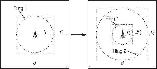
Figure 3.6 Illustration of rings.
Once virtual rings are established, gateways can be distributed on the rings. On each ring, the gateways are roughly ![]() away from each other; therefore, the maximum number of gateways on a ring
away from each other; therefore, the maximum number of gateways on a ring ![]() is as follows:
is as follows:
One may have realized that not all gateways are guaranteed to be deployed on the virtual rings evenly. Thus we determine the number of gateways on each ring first and then deploy them on each ring. Let ![]() be the set of distances from gateways to the concentrator. Each distance
be the set of distances from gateways to the concentrator. Each distance ![]() reveals the ring that gateway
reveals the ring that gateway ![]() is deployed. We propose two methods to find the set of distances
is deployed. We propose two methods to find the set of distances ![]() .
.
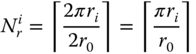
In the first method, gateways are deployed one on each ring, starting from the outermost ring. The maximum number of gateways on each ring is determined by ![]() . Using
. Using ![]() and d = 1 km, the deployment is illustrated in Figure 3.7. The gateway DAPs are deployed along two virtual rings, where the outer ring has six and the inner ring has two.
and d = 1 km, the deployment is illustrated in Figure 3.7. The gateway DAPs are deployed along two virtual rings, where the outer ring has six and the inner ring has two.

Figure 3.7 Illustration of “one on each” method.
In the second method, each ring is fully deployed on a virtual ring before moving onto the next ring, starting from the outermost ring. As shown in Figure 3.8, the deployment is different from that using the first method. While the gateway DAPs are also deployed along two virtual rings, the second method deploys just one on the inner ring. Apparently, the outsider ring first method will provide a better level of fairness to the customers that are further away from the concentrator. However, more gateways on the outsider rings have side effects on the uplink transmission performance, which will be discussed later in this chapter.
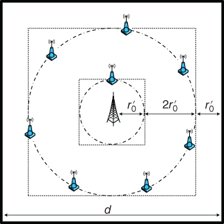
Figure 3.8 Illustration of “outsider ring first” method.
3.3.4 Global Uplink Transmission Power Efficiency
Many researches have considered individual power efficiency (e.g. for DAP ![]() ,
, ![]() (bits/joule)) for each node in a multiaccess system. Most of them applied noncooperative game theoretical approaches where each player achieves its maximum power efficiency selfishly. However, that approach cannot achieve the maximum social welfare (or the global uplink transmission power efficiency). The global power efficiency is defined as the ratio of total effective uplink transmission rate to the total transmission power. With a given topology for gateway DAPs, the problem is described as follows:
(bits/joule)) for each node in a multiaccess system. Most of them applied noncooperative game theoretical approaches where each player achieves its maximum power efficiency selfishly. However, that approach cannot achieve the maximum social welfare (or the global uplink transmission power efficiency). The global power efficiency is defined as the ratio of total effective uplink transmission rate to the total transmission power. With a given topology for gateway DAPs, the problem is described as follows:

such that
and
Constraint Eq. (3.41) indicates that the transmitting power ![]() for each gateway has an upper bound imposed by the FCC rules (especially using ISM bands). Constraint Eq. (3.42) is for the fairness. As discussed before, all gateway DAPs shall have the same receiving power at the concentrator. Without this fairness constraint, this nonlinear optimization problem has
for each gateway has an upper bound imposed by the FCC rules (especially using ISM bands). Constraint Eq. (3.42) is for the fairness. As discussed before, all gateway DAPs shall have the same receiving power at the concentrator. Without this fairness constraint, this nonlinear optimization problem has ![]() extra parameters (
extra parameters (![]() ) and would thus be harder to solve. Nonetheless, with fairness introduced, there is only one parameter
) and would thus be harder to solve. Nonetheless, with fairness introduced, there is only one parameter ![]() to optimize, which reduces the complexity of the problem.
to optimize, which reduces the complexity of the problem.
Although the traditional noncooperative game theoretical approach did not have the constraint of equal ![]() , its Nash equilibrium was derived with a uniform
, its Nash equilibrium was derived with a uniform ![]() such that
such that ![]() [72–75]. In practice, maximizing individual power efficiency cannot achieve global power efficiency. Assuming
[72–75]. In practice, maximizing individual power efficiency cannot achieve global power efficiency. Assuming ![]() , the relationship between global power efficiency and receiving SINR
, the relationship between global power efficiency and receiving SINR ![]() as well as the relationship between global transmission rate and
as well as the relationship between global transmission rate and ![]() are illustrated in Figure 3.9. From the figure we can see that:
are illustrated in Figure 3.9. From the figure we can see that:
- The global transmission rate increases with respect to SINR. However, the marginal increase will decrease as SINR goes higher.
- A maximizer of the global power efficiency exists. The maximizer does not necessarily represent the optimal SINR that can support the data transmission rate.
- The maximizer achieved by noncooperative game theoretical approach will be off from the global maximizer. It requires a higher SINR, which benefits the transmission rate.
Figure 3.9 Global uplink transmission power efficiency.
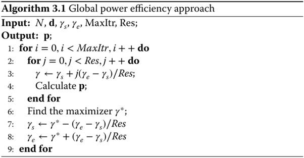
To find optimal solution to global power efficiency, we propose an algorithm as illustrated in Algorithm 3.1. Let ![]() be the set of power usages of each DAP. Let
be the set of power usages of each DAP. Let ![]() be the number of iterations, and
be the number of iterations, and ![]() be the resolution of each iteration. In each iteration starting from
be the resolution of each iteration. In each iteration starting from ![]() and ending at
and ending at ![]() , there is one maximizer
, there is one maximizer ![]() to be found. In the next iteration, the algorithm updates
to be found. In the next iteration, the algorithm updates ![]() and
and ![]() . With a given
. With a given ![]() , the computational complexity depends on calculating
, the computational complexity depends on calculating ![]() . Fortunately, calculating
. Fortunately, calculating ![]() is indeed solving a linear equation system of
is indeed solving a linear equation system of ![]() linear equations with
linear equations with ![]() unknowns. Its computational complexity has an upper bound at
unknowns. Its computational complexity has an upper bound at ![]() when applying Strassen's algorithm [77] for matrix multiplication. Therefore, Algorithm 3.1 has an upper bound for computational complexity
when applying Strassen's algorithm [77] for matrix multiplication. Therefore, Algorithm 3.1 has an upper bound for computational complexity ![]() , where
, where ![]() .
.
3.4 Numerical Results
In this section, we evaluate the formulated problems and the corresponding solutions with simulations.
3.4.1 Evaluation of the Optimal Number of Gateways
Let the noise ![]() dBm, M=100 bits, and
dBm, M=100 bits, and ![]() . Assume a neighborhood block with
. Assume a neighborhood block with ![]() km. We first show the maximum number of gateway DAPs with respect to different maximum receiving power
km. We first show the maximum number of gateway DAPs with respect to different maximum receiving power ![]() . Given a
. Given a ![]() , an optimal number of gateway DAPs can be found by the solution given in the previous section. As shown in Figure 3.10, with higher
, an optimal number of gateway DAPs can be found by the solution given in the previous section. As shown in Figure 3.10, with higher ![]() , the optimal
, the optimal ![]() is higher. However, as discussed before, deploying more gateway DAPs causes lower
is higher. However, as discussed before, deploying more gateway DAPs causes lower ![]() since we need to achieve geographical fairness. Therefore, it cannot deploy too many gateway DAPs while applying low
since we need to achieve geographical fairness. Therefore, it cannot deploy too many gateway DAPs while applying low ![]() .
.

Figure 3.10 Optimal number of gateways.
3.4.2 Evaluation of the Global Power Efficiency
The global power efficiency depends on the number as well as the deployment of gateway DAPs. The proposed centralized optimization and the traditional game theoretical approach may achieve different results. In the evaluation, geographical issues are considered is only for the centralized approach, since the game theoretical approach is independent of actual deployment as long as the concentrator can still receive from the furthest gateway DAP at optimal SINR.
Figure 3.11 shows the global power efficiency in bits/joule. In general, the global power efficiency decreases as the number of gateway DAPs increases. From the figure we can see that when ![]() , all four approaches considering geographical deployment have a sudden drop in global power efficiency. This is caused by the addition of an extra virtual ring in the deployment. Apparently, there is no sudden performance drop without a concern for geographical fairness. Also, no geographical concern appears to have the highest global power efficiency. This occurs because all the gateway DAPs are deployed at closer distances to the concentrator. In reality, we shall adopt the geographical deployment to achieve fairness. Among the four approaches considering geographical deployment, both of the game theoretical approaches achieve lower global power efficiency compared with the centralized optimization results. The centralized optimization results of two deployments appear to be the same, because the deployments are the same for both deployment methods when
, all four approaches considering geographical deployment have a sudden drop in global power efficiency. This is caused by the addition of an extra virtual ring in the deployment. Apparently, there is no sudden performance drop without a concern for geographical fairness. Also, no geographical concern appears to have the highest global power efficiency. This occurs because all the gateway DAPs are deployed at closer distances to the concentrator. In reality, we shall adopt the geographical deployment to achieve fairness. Among the four approaches considering geographical deployment, both of the game theoretical approaches achieve lower global power efficiency compared with the centralized optimization results. The centralized optimization results of two deployments appear to be the same, because the deployments are the same for both deployment methods when ![]() except for
except for ![]() .
.
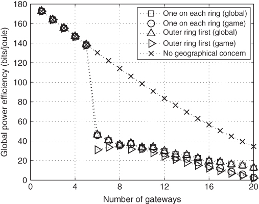
Figure 3.11 Global power efficiency with respect to number of gateways.
3.4.3 Evaluation of the Global Uplink Transmission Rates
In this evaluation, we show the global uplink transmission rates achieved by the proposed approach in comparison to the results achieved by the traditional game theoretical approach.
The results are shown in Figure 3.12. As we can see, the proposed centralized optimization approaches, denoted by “global” in the figure, would achieve the same results regardless of geographical deployments. It is because the global uplink transmission rate depends solely on ![]() given the number of gateway DAPs. As long as the furthest gateway DAP is able to achieve
given the number of gateway DAPs. As long as the furthest gateway DAP is able to achieve ![]() with the same
with the same ![]() , the global uplink transmission rate will remain the same. As a comparison, the global uplink transmission rates achieved by the traditional game theoretical approach are higher than those achieved by centralized optimization. This is due to the higher
, the global uplink transmission rate will remain the same. As a comparison, the global uplink transmission rates achieved by the traditional game theoretical approach are higher than those achieved by centralized optimization. This is due to the higher ![]() achieving Nash equilibrium in game theoretical approaches (as shown earlier in Figure 3.9). While not shown in this figure, even the game theoretical approach will have a decreasing marginal increase in the global transmission rate. More importantly, we can see that a maximizer exists when applying global optimization. Therefore, an optimal number of gateway DAPs can be determined accordingly. The results also show that if increased service is needed for more customers, the NAN uplink transmission performance can be enhanced easily by increasing transmission power of each gateway DAP. There is no need for a hardware upgrade in this structure.
achieving Nash equilibrium in game theoretical approaches (as shown earlier in Figure 3.9). While not shown in this figure, even the game theoretical approach will have a decreasing marginal increase in the global transmission rate. More importantly, we can see that a maximizer exists when applying global optimization. Therefore, an optimal number of gateway DAPs can be determined accordingly. The results also show that if increased service is needed for more customers, the NAN uplink transmission performance can be enhanced easily by increasing transmission power of each gateway DAP. There is no need for a hardware upgrade in this structure.

Figure 3.12 Global transmission rate with respect to number of gateways.
3.4.4 Evaluation of the Global Power Consumption
In this evaluation, we show the global power consumption of the gateway DAPs with different approaches. The results are given in Figure 3.13.

Figure 3.13 Global power consumption with respect to number of gateways.
We can see that with no geographical consideration, the global power consumption is the lowest. This is because when no deployment issue is considered, the gateway DAPs are actually deployed closer to the concentrator, resulting in lower power consumption. Moreover, the game theoretical approaches have slight higher global power consumption due to their correspondingly higher ![]() .
.
3.4.5 Evaluation of the Minimum Cost Problem
The solution to the minimum cost problem is to find the sufficient size of solar panel and capacity of battery for each DAP to survive the designed life cycle. The transmission power ![]() of a gateway DAP is determined by solving the maximum global power efficiency problem after finding the optimal number of gateway DAPs. The transmission power of a normal DAP is a constant value set for Wi‐Fi transmissions. With a given transmission power
of a gateway DAP is determined by solving the maximum global power efficiency problem after finding the optimal number of gateway DAPs. The transmission power of a normal DAP is a constant value set for Wi‐Fi transmissions. With a given transmission power ![]() , the key factors of the minimum cost problem are the length of life cycle
, the key factors of the minimum cost problem are the length of life cycle ![]() as well as the estimated worst‐case scenario
as well as the estimated worst‐case scenario ![]() . This evaluation is to show the relationships between those factors. Without loss of generality, let
. This evaluation is to show the relationships between those factors. Without loss of generality, let ![]() ,
, ![]() per Wh, and
per Wh, and ![]() per unit solar panel for the maximum 1 W charging rate. With
per unit solar panel for the maximum 1 W charging rate. With ![]() , evaluation is performed with
, evaluation is performed with ![]() . In addition to that, when
. In addition to that, when ![]() , evaluation is also performed with
, evaluation is also performed with ![]() . Different settings can be easily applied to set other benchmark evaluations.
. Different settings can be easily applied to set other benchmark evaluations.
First, we evaluate the impact on total cost (the objective function) with respect to different values of ![]() . The results are given in Figure 3.14. As we can see, either higher
. The results are given in Figure 3.14. As we can see, either higher ![]() or higher
or higher ![]() will increase total cost for a DAP, since it will need a larger battery and larger solar panel to be self‐sustaining over a longer and harsher life cycle.
will increase total cost for a DAP, since it will need a larger battery and larger solar panel to be self‐sustaining over a longer and harsher life cycle.
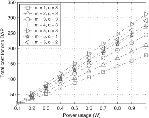
Figure 3.14 Total cost of a DAP.
Then, we evaluate the impact on battery capacity with respect to different values of ![]() . The results are given in Figure 3.15. As we can see, a larger battery is required with a longer life cycle and higher transmission power.
. The results are given in Figure 3.15. As we can see, a larger battery is required with a longer life cycle and higher transmission power.
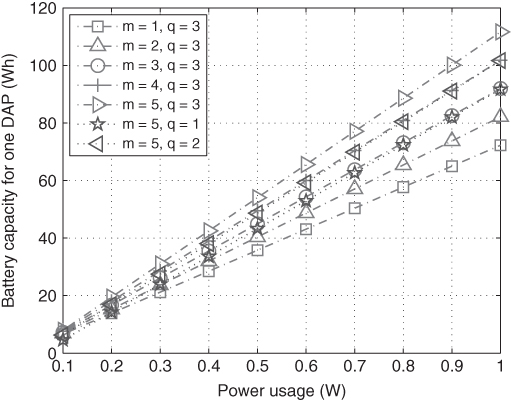
Figure 3.15 Battery capacity of a DAP.
The impact on solar panel size is shown in Figure 3.16. Note that the solar panel size is the same when ![]() and
and ![]() . Although the battery capacities are different, the charging rate is high enough to handle the situations.
. Although the battery capacities are different, the charging rate is high enough to handle the situations.

Figure 3.16 Solar panel size of a DAP.
Finally, we show the impact on charging threshold in Figure 3.17. As it shows, with a higher ![]() , the charging threshold increases. However, with a higher
, the charging threshold increases. However, with a higher ![]() , the charging threshold decreases. On one hand, more capacity remaining in the battery is required to survive a longer period with bad weather. On the other hand, if the required life cycle is longer, then the battery must reduce its charging frequency to slow down the deterioration of that battery.
, the charging threshold decreases. On one hand, more capacity remaining in the battery is required to survive a longer period with bad weather. On the other hand, if the required life cycle is longer, then the battery must reduce its charging frequency to slow down the deterioration of that battery.

Figure 3.17 Impact on charging thresholds of a DAP.
3.5 Case Study
In this section, we present a case study to demonstrate the self‐sustainability of the proposed NAN design with the results from previous evaluations. In the case study, the neighborhood has a dimension of d=1 km. The optimal number of gateway DAPs in this neighborhood is 18. Both of the deployment methods will have the gateway DAPs placed in the same place. The furthest gateway DAP (i.e. DAP ![]() ) operates at
) operates at ![]() mW to achieve maximum global power efficiency. Assume that the NAN is designed for
mW to achieve maximum global power efficiency. Assume that the NAN is designed for ![]() years and
years and ![]() . The optimal settings of each battery and solar panel are
. The optimal settings of each battery and solar panel are ![]() ,
, ![]() , and
, and ![]() . The weather conditions are assumed to be random throughout a year but remain constant in a day for simplicity. The NAN is evaluated with different probabilities of sunny weather.
. The weather conditions are assumed to be random throughout a year but remain constant in a day for simplicity. The NAN is evaluated with different probabilities of sunny weather.
First, we show the remaining energy at sunrise on each day in Figure 3.18 with a ![]() probability of sunny weather. From the results, we can see that the exact battery capacity drops below the original capacity as time passes due to deterioration. It also shows that no charging begins when
probability of sunny weather. From the results, we can see that the exact battery capacity drops below the original capacity as time passes due to deterioration. It also shows that no charging begins when ![]() ; however, charging may not begin not only below the charging threshold, but also when
; however, charging may not begin not only below the charging threshold, but also when ![]() due to continuous cloudy days. Sometimes, the battery could be charged just before it gets completely depleted. One may use a slightly larger capacity or higher charging threshold to enhance self‐sustainability.
due to continuous cloudy days. Sometimes, the battery could be charged just before it gets completely depleted. One may use a slightly larger capacity or higher charging threshold to enhance self‐sustainability.
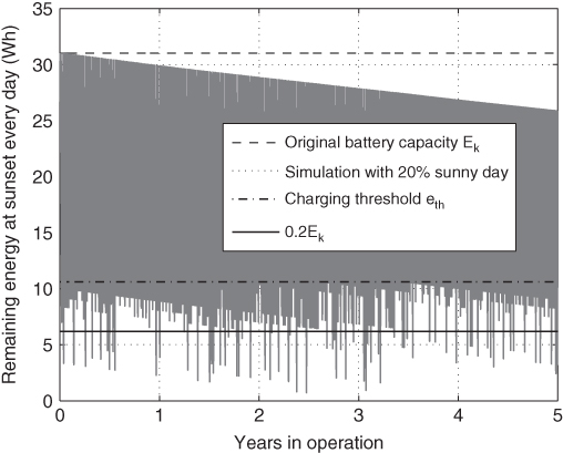
Figure 3.18 Remaining energy at  every day.
A closer look at ![]() is shown in Figure 3.19. With a higher probability of sunny weather, the
is shown in Figure 3.19. With a higher probability of sunny weather, the ![]() is lower. A simple explanation is that a larger number of sunny days makes the DAP more likely to activate a charger right after the remaining energy hits the threshold and thus causes more charging cycles. Although the
is lower. A simple explanation is that a larger number of sunny days makes the DAP more likely to activate a charger right after the remaining energy hits the threshold and thus causes more charging cycles. Although the ![]() after each charge depends on the corresponding
after each charge depends on the corresponding ![]() , the
, the ![]() in this case are more than
in this case are more than ![]() when
when ![]() is close to 500. Therefore the approximation is reliable. Note that the final
is close to 500. Therefore the approximation is reliable. Note that the final ![]() of all situations are below
of all situations are below ![]() and thus this battery will survive throughout five years. Different settings can be applied before actual deployment of a NAN for better self‐sustainability.
and thus this battery will survive throughout five years. Different settings can be applied before actual deployment of a NAN for better self‐sustainability.

Figure 3.19 at
at  every day.
3.6 Summary
In this chapter, we proposed an energy‐efficient, self‐sustaining wireless NAN design that is powered by a solar panel. We proposed a centralized optimization method so that the cost of the NAN can be minimized. In order to find the solution, we discussed the optimal number of gateway DAPs. We also applied two geographical deployment algorithms so that the fairness of high‐quality service can be achieved for all the customers, especially ones farther from the concentrator. When determining the transmission power of each gateway DAP, we tailored the approach for global power efficiency instead of individual power efficiency. Compared with the traditional game theoretical approach, our proposed approach can achieve lower power usage and higher power efficiency. The case study demonstrated that our design is self‐sustaining.