
Chapter 11: Using Pachyderm Notebooks
In Chapter 10, Pachyderm Language Clients, we learned how to use Pachyderm language clients, including the Pachyderm Go client and Pachyderm Python client. The latter is probably more popular among data scientists as Python is the language that a lot of data scientists use. And if you write in Python, you are likely familiar with the open source tool, JupyterLab.
JupyterLab is an open source platform that provides an Interactive Development Environment (IDE) in which you can not only author your code but also execute it. This advantage makes JupyterLab an ideal tool for data science experiments. However, while JupyterLab provides a basic version control system for its notebooks, it's not to the level of data provenance that Pachyderm offers. Pachyderm Hub, the SaaS version of Pachyderm, provides a way to integrate your Pachyderm cluster with Pachyderm Notebooks, a built-in version of JupyterLab coupled with Pachyderm.
This chapter is intended to demonstrate how to configure a Pachyderm cluster in Pachyderm Hub and use Pachyderm Notebooks. By the end of this chapter, we will learn how to run basic Pachyderm operations in Pachyderm Notebooks and will create a sentiment analysis pipeline.
This chapter covers the following topics:
- Enabling Pachyderm Notebooks in Pachyderm Hub
- Running basic Pachyderm operations in Pachyderm Notebooks
- Creating and running an example pipeline in Pachyderm Notebooks
Technical requirements
You should have already installed the following components:
- pachctl 2.0.0 or later
- Access to Pachyderm Hub
- A GitHub or Gmail account
Downloading the source files
All code samples used in this section are stored in the GitHub repository created for this book at https://github.com/PacktPublishing/Reproducible-Data-Science-with-Pachyderm/tree/main/Chapter11-Using-Pachyderm-Notebooks.
The Dockerfile used in this section is stored at https://hub.docker.com/repository/docker/svekars/pachyderm-ide.
Enabling Pachyderm Notebooks in Pachyderm Hub
Before you can take advantage of Pachyderm Notebooks, you need to create an account in Pachyderm Hub and a Pachyderm workspace. Pachyderm Hub provides a trial period for all users to test its functionality.
After the trial period ends, you need to upgrade to the Pachyderm Pro version to continue using Pachyderm Notebooks.
Create a workspace
In Pachyderm Hub, your work is organized in workspaces. A workspace is a grouping in which multiple Pachyderm clusters can run. Your organization might decide to assign each workspace to a team of engineers.
Before you can create a workspace, you need a Pachyderm Hub account, so let's create one. Pachyderm Hub supports authentication with Gmail and GitHub. You must have either of those to create an account with Pachyderm Hub.
To create a Pachyderm Hub account, complete the following steps:
- Go to https://www.pachyderm.com/try-pachyderm-hub# and fill out the provided form to request a free trial of Pachyderm Hub. It might take some time for your account to be activated and you will receive an email with instructions.
- Log in to your Pachyderm Hub account with the Gmail or GitHub account you have provided in the sign-up form.
- Fill out the Get Started form and click Get Started.
- Click Create a workspace, fill out the form that appears as shown in the following screenshot, and click Create:

Figure 11.1 – Create a new workspace
When you create a workspace, you automatically deploy a Pachyderm cluster. If you're using a trial version of Pachyderm, you will have deployed a single-node cluster, which should be enough for testing.
Now that you have created your first workspace, you need to connect to your cluster using pachctl.
Connect to your Pachyderm Hub workspace with pachctl
If this is not the first chapter that you are reading in this book, you should already have pacthl installed on your computer. Otherwise, install pachctl as described in Chapter 4, Installing Pachyderm Locally.
To connect to your Pachyderm Hub workspace, do the following:
- In the Pachyderm Hub UI, locate your workspace, and click the CLI link.
- Follow the instructions in the UI to switch your Pachyderm context and enable communication between your computer and your workspace on Pachyderm Hub.
- After you authenticate, run the following command:
pachctl version
You should get the following response:
COMPONENT VERSION
pachctl 2.0.1
pachd 2.0.1
- Check that you have switched to the correct context by running the following command:
pachctl config get active-context
This command should return the name of your Pachyderm Hub workspace.
You can now communicate with your cluster deployed on Pachyderm Hub through pachctl from a terminal on your computer.
Now that we have configured our cluster, let's connect to a Pachyderm notebook.
Connect to a Pachyderm notebook
Pachyderm Notebooks is an IDE for data scientists that provides easy access to familiar Python libraries. You can run and test your code in cells while Pachyderm backs your pipeline.
To connect to a Pachyderm notebook, complete the following steps:
- In the Pachyderm Hub UI, in your workspace, click Notebooks:

Figure 11.2 – Access Pachyderm Notebooks
- When prompted, click Sign in with OAuth 2.0 and then sign in with the account that has access to Pachyderm Hub.
- On the Server Options screen, select the Default server:
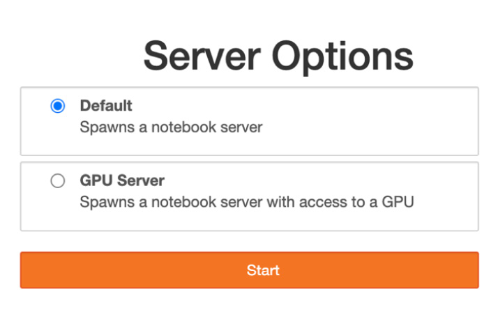
Figure 11.3 – Server Options
- Click Start and then Launch Server.
You should see the following screen:
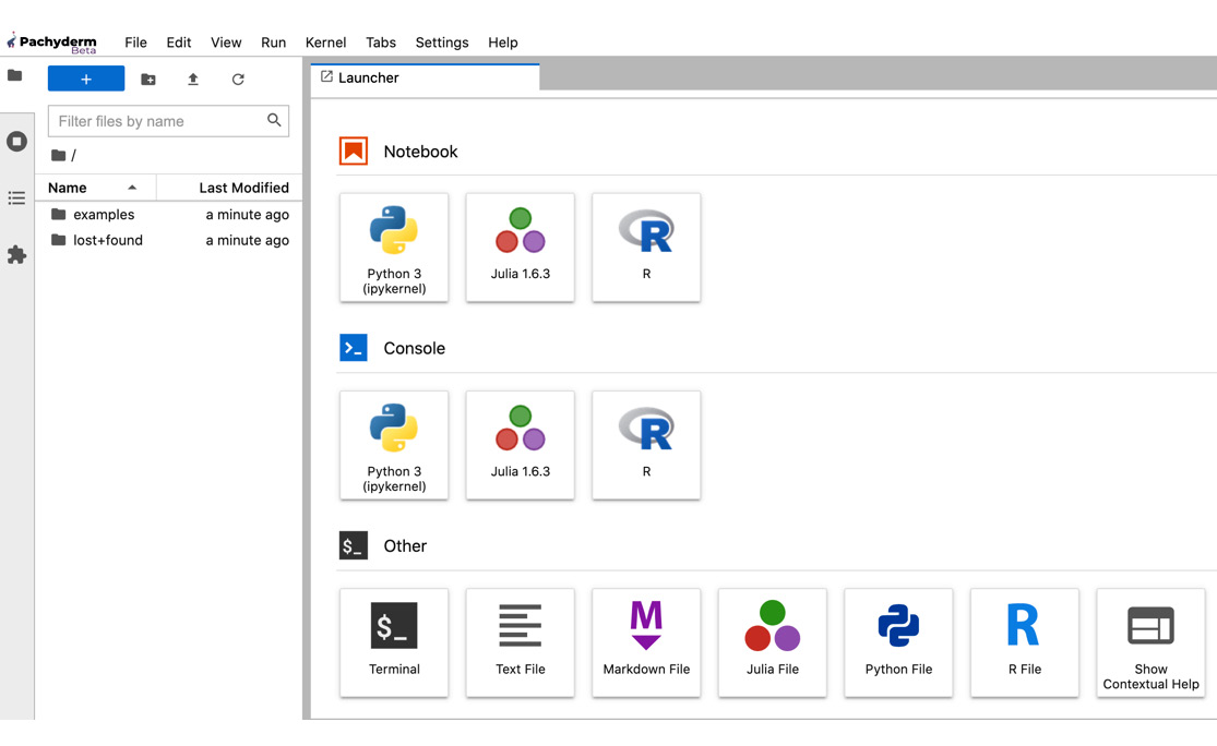
Figure 11.4 – Pachyderm Notebooks home
Now that we have access to Pachyderm Notebooks, we can create Pachyderm pipelines directly from the Pachyderm Notebooks UI, experiment with Python code and python-pachyderm, run pachctl commands, and even create Markdown files to document our experiments. We'll look into this functionality in the next section.
Running basic Pachyderm operations in Pachyderm Notebooks
The main advantage of Pachyderm Notebooks is that it provides a unified experience. Not only can you run your experiments inside of it, but you can also access your Pachyderm cluster through the integrated terminal by using both pachctl and python-pachyderm. All the pipelines that you create through the JupyterLab UI will be reflected in your Pachyderm cluster whether it runs locally or on a cloud platform.
Now let's see how we can use Pachyderm Notebooks to access our Pachyderm cluster.
Using the integrated terminal
You can run the integrated terminal from within Pachyderm Notebooks and use it to execute pachctl or any other UNIX commands.
To use the integrated terminal, complete the following steps:
- On the Pachyderm Notebooks home page, click Terminal.
- Click the Terminal icon to start a new Terminal window:

Figure 11.5 – Start a Terminal within Pachyderm Notebooks
- Get the version of Pachyderm:
pachctl version
Try running other Pachyderm commands that you have learned in previous chapters to see how it works.
Important note
The version of pachctl and pachd are different than the ones your run directly from your computer terminal as Pachyderm Notebooks has a preinstalled version of pachctl, which sometimes might not match the version of your cluster. This should not affect your work with Pachyderm.
Now that we know how to use the terminal, let's try to create a Pachyderm notebook.
Using Pachyderm Notebooks
A notebook is an interactive document in which the users can write Python code, run it, and visualize it. These features make notebooks a great experimentation tool that many data scientists use in their work. After the experiment is finished, you might want to export the notebook as a Python script or library.
Pachyderm Notebooks supports the following types of notebooks:
- Python notebooks
- Julia notebooks
- R notebooks
These three languages seem to be most popular among data scientists. You can create Julia and R notebooks to experiment specifically with the code that you want to use with your pipeline. With Python notebooks, not only you can test your code, but you can also use the python-pachyderm client to interact with the Pachyderm cluster.
Important note
The code described in this section can be found in the https://github.com/PacktPublishing/Reproducible-Data-Science-with-Pachyderm/blob/main/Chapter11-Using-Pachyderm-Notebooks/example.ipynb file.
Let's create a Python notebook and run a few commands:
- On the Pachyderm Notebooks home screen, click on the Python 3 notebook icon to create a new notebook.
- We can use both regular Python and python-pachyderm in this notebook. For example, to get the current version of your Pachyderm cluster and list all the repositories, paste the following in the notebook's cell:
import python_pachyderm
client = python_pachyderm.Client()
print(client.get_remote_version())
print(list(client.list_repo()))
- Click the run icon to run the script and get the result:

Figure 11.6 – Running python-pachyderm in Notebooks
- Create a repository by pasting the following code in the next cell and running it:
client.create_repo("data")
print(list(client.list_repo()))
Here is the output that you should see:

Figure 11.7 – List repo
Note that you do not need to import python_pachyderm and define the client in the second and subsequent cells since you have already defined it in the first cell.
- Let's add some files to the data repository:
with client.commit('data', 'master') as i:
client.put_file_url(i, 'total_vaccinations_dec_2020_24-31.csv', 'https://raw.githubusercontent.com/PacktPublishing/Reproducible-Data-Science-with-Pachyderm/main/Chapter11-Using-Pachyderm-Notebooks/total_vaccinations_dec_2020_24-31.csv')
print(list(client.list_file(("data", "master"), "")))
Here is the output that you should see:

Figure 11.8 – Put file output
This dataset contains statistics about COVID-19 vaccinations from December 24 to 31, 2020.
- You can print the contents of the file by running the following code:
import pandas as pd
pd.read_csv(client.get_file(("data", "master"), "total_vaccinations_dec_2020_24-31.csv"))
You should see the following output:

Figure 11.9 – Total vaccinations
This CSV file has the following columns: location, date, vaccine (manufacturer), and total_vaccinations.
- Let's also print the top five rows of the file to view the names of the columns:
import pandas as pd
df = pd.read_csv(client.get_file(("data", "master"), "total_vaccinations_dec_2020_24-31.csv"))
data_top = df.head()
print(data_top)
You should see the following output:
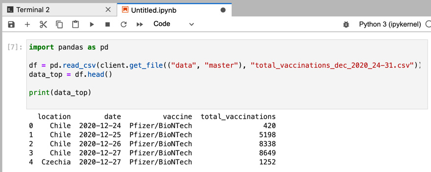
Figure 11.10 – Top five rows
- Finally, let's create a simple pipeline that will tell us which country did the most vaccinations in a single given day during the observed period:
from python_pachyderm.service import pps_proto
client.create_pipeline(
pipeline_name="find-vaccinations",
transform=pps_proto.Transform(
cmd=["python3"],
stdin=[
"import pandas as pd",
"df = pd.read_csv('/pfs/data/total_vaccinations_dec_2020_24-31.csv')",
"max_vac = df['total_vaccinations'].idxmax()",
"row = df.iloc[[max_vac]]",
"row.to_csv('/pfs/out/max_vaccinations.csv', header=None, index=None, sep=' ', mode='a')",
],
image="amancevice/pandas",
),
input=pps_proto.Input(
pfs=pps_proto.PFSInput(glob="/", repo="data")
),
)
print(list(client.list_pipeline()))
You should see the following output:

Figure 11.11 – Create pipeline output
- Let's get the result of our pipeline by executing the following code:
client.get_file(("find-vaccinations", "master"), "/max_vaccinations.csv").read()
You should see the following output:
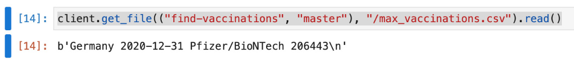
Figure 11.12 – Results of the pipeline
Our pipeline has determined that during the period from December 24 to December 31, the most vaccinations were done in Germany on December 31. The number of vaccinations was 206443 and the manufacturer was Pfizer/BioNTech.
- To clean up your cluster, run the following:
client.delete_repo("data", force=True)
client.delete_pipeline("find-vaccinations")
print(list(client.list_repo()))
print(list(client.list_pipeline()))
You should see the following output:
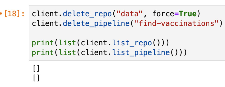
Figure 11.13 – Cluster clean up
In this section, we learned how to perform basic Pachyderm operations in Pachyderm Python Notebooks. Next, we'll create another example pipeline.
Creating and running an example pipeline in Pachyderm Notebooks
In the previous section, we learned how to use Pachyderm Notebooks, create repositories, put data, and even created a simple pipeline. In this section, we will create a pipeline that performs sentiment analysis on a Twitter dataset.
Important note
The code described in this section can be found in the https://github.com/PacktPublishing/Reproducible-Data-Science-with-Pachyderm/blob/main/Chapter11-Using-Pachyderm-Notebooks/sentiment-pipeline.ipynb file.
We will use a modified version of the International Women's Day Tweets dataset from Kaggle available at https://www.kaggle.com/michau96/international-womens-day-tweets. Our modified version includes only two columns—tweet number # and text. The dataset includes 51,480 rows.
Here is an extract of the first few rows of the dataset:
# text
0 3 "She believed she could, so she did." #interna...
1 4 Knocking it out of the park again is @marya...
2 5 Happy International Women's Day! Today we are ...
3 6 Happy #InternationalWomensDay You're all power...
4 7 Listen to an experimental podcast recorded by ...
Here is a diagram of the workflow:

Figure 11.14 – Sentiment analysis pipeline
In the next section, we will learn about the methodology that is used to build this pipeline.
Pipeline methodology
We will use Natural Language Toolkit (NLTK), which is familiar to us from previous chapters, to clean the data. Then, we will use TextBlob, an open source Python library for text processing, to perform sentiment analysis on the tweets in the dataset.
Sentiment analysis is a technique that helps understand the overall mood of the individuals involved in a specific conversation, discussing specific products and services, or rating a movie. Sentiment analysis is widely used in various types of businesses and industries by marketers and sociologists to get a quick assessment of customer sentiment. In this example, we will be looking at emotions expressed in a selection of tweets about International Women's Day.
TextBlob provides two metrics for sentiment analysis—polarity and subjectivity. Each word in a sentence is assigned a score and then the mean score is assigned to the whole sentence. In this example, we will only determine the polarity of the tweets. Polarity defines the positivity or negativity of a sentence based on a predefined word intensity.
Polarity values range from -1 to 1, with -1 meaning negative sentiment, 0 being neutral, and 1 being positive. If we were to show this on a scale, it would look like this:

Figure 11.15 – Polarity
If we were to put the words into a table and assign them polarity scores, here is what we might get:

Figure 11.16 – Polarity scores
Let's run a quick TextBlob example on a simple sentence to see how it works. Use the code in the sentiment-test.py file to try this example:
from textblob import TextBlob
text = '''Here is the most simple example of a sentence. The rest of the text is autogenerated. This gives the program some time to perform its computations and then tries to find the shortest possible possible sentence. Finally, let's look at the output that is used for the rest of the process.'''
blob = TextBlob(text)
blob.tags
blob.noun_phrases
for i in blob.sentences:
print(i.sentiment.polarity)
To run this script, complete the following steps:
- You need to install TextBlob in the Pachyderm Notebooks terminal:
pip install textblob && python -m textblob.download_corpora
Here is the output that you should see:

Figure 11.17 – Installing TextBlob

Figure 11.18 – Output of the sentiment-test.py script
As you can see in the output, TextBlob assigns a score for each sentence.
Now that we have reviewed the methodology of our example, let's create our pipelines.
Creating the pipelines
Our first pipeline will use NLTK to clean the Twitter data in our data.csv file. We will create a standard Pachyderm pipeline by using python-pachyderm. The pipeline will consume files from the data repository, run the data-clean.py script on it, and output the cleaned text to the data-clean output repository. The pipeline will use the svekars/pachyderm-ide:1.0 Docker image to run the code.
The first part of data-clean.py imports the components that are familiar to us from Chapter 8, Creating an End-to-End Machine Learning Workflow. These components include NLTK and pandas, which we will use to preprocess our data. We will also import re to specify regular expressions:
import nltk
import pandas as pd
from nltk.corpus import stopwords
from nltk.tokenize import word_tokenize
nltk.download('wordnet')
nltk.download('punkt')
import re
The second part of the script performs the data cleaning using the NLTK word_tokenize method, stopwords with the lambda function, and re.split to remove the URLs. Finally, the script saves the cleaned text to cleaned-data.csv in the output repository:
stopwords = stopwords.words("english")
data = pd.read_csv("/pfs/data/data.csv", delimiter=",")
tokens = data['text'].apply(word_tokenize)
remove_stopwords = tokens.apply(lambda x: [w for w in x if w not in stopwords and w.isalpha()])
remove_urls = remove_stopwords.apply(lambda x: re.split('https://.*', str(x))[0])
remove_urls.to_csv('/pfs/out/cleaned-data.csv', index=True)
Our second pipeline will perform sentiment analysis on the cleaned data with the TextBlob Python library. The sentiment.py script imports the following components:
from textblob import TextBlob
import pandas as pd
import seaborn as sns
import matplotlib.pyplot as plt
from contextlib import redirect_stdout
We'll use pandas to manipulate the data frames. We'll use matplotlib and seaborn to visualize our results, and we'll use redirect_stdout to save our results to a file.
Next, our script performs sentiment analysis and creates two new columns—polarity_score and sentiment. The resulting table is saved to a new CSV file called polarity.csv:
data = pd.read_csv('/pfs/data-clean/cleaned-data.csv', delimiter=',')
data = data[['text']]
data["polarity_score"] = data["text"].apply(lambda data: TextBlob(data).sentiment.polarity)
data['sentiment'] = data['polarity_score'].apply(lambda x: 'Positive' if x >= 0.1 else ('Negative' if x <= -0.1 else 'Neutral'))
print(data.head(10))
data.to_csv('/pfs/out/polarity.csv', index=True)
Then, the script saves the tweets of sentiment category to its own variable, calculates the total for each category, and saves the totals to the number_of_tweets.txt file:
positive = [ data for index, t in enumerate(data['text']) if data['polarity_score'][index] > 0]
neutral = [ data for index, tweet in enumerate(data['text']) if data['polarity_score'][index] == 0]
negative = [ data for index, t in enumerate(data['text']) if data['polarity_score'][index] < 0]
with open('/pfs/out/number_of_tweets.txt', 'w') as file:
with redirect_stdout(file):
print("Number of Positive tweets:", len(positive))
print("Number of Neutral tweets:", len(neutral))
print("Number of Negative tweets:", len(negative))
The last part of the script builds a pie chart with the percentages of tweets in each category and saves them to the plot.png file:
colors = ['#9b5de5','#f15bb5','#fee440']
figure = pd.DataFrame({'percentage': [len(positive), len(negative), len(neutral)]},
index=['Positive', 'Negative', 'Neutral'])
plot = figure.plot.pie(y='percentage', figsize=(5, 5), autopct='%1.1f%%', colors=colors)
circle = plt.Circle((0,0),0.70,fc='white')
fig = plt.gcf()
fig.gca().add_artist(circle)
plot.axis('equal')
plt.tight_layout()
plot.figure.savefig("/pfs/out/plot.png")
- Create a new Pachyderm Python notebook.
- Create a Pachyderm data repository:
import python_pachyderm
client = python_pachyderm.Client()
client.create_repo("data")
print(list(client.list_repo()))
You should see the following output:

Figure 11.19 – Output of the created repository
- Put the data.csv file in this repository:
with client.commit('data', 'master') as i:
client.put_file_url(i, 'data.csv', 'https://raw.githubusercontent.com/PacktPublishing/Reproducible-Data-Science-with-Pachyderm/main/Chapter11-Using-Pachyderm-Notebooks/data.csv')
print(list(client.list_file(("data", "master"), "")))
This script returns the following output:
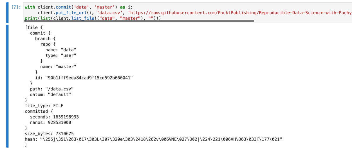
Figure 11.20 – Put file output
- List the files in the data repository:
list(client.list_file(("data", "master"), ""))
You should see the following response:
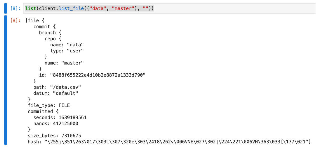
Figure 11.21 – List file output
- Create the data-clean pipeline:
from python_pachyderm.service import pps_proto
client.create_pipeline(
pipeline_name="data-clean",
transform=pps_proto.Transform(
cmd=["python3", "data-clean.py"],
image="svekars/pachyderm-ide:1.0",
),
input=pps_proto.Input(
pfs=pps_proto.PFSInput(glob="/", repo="data")
),
)
client.create_pipeline(
pipeline_name="sentiment",
transform=pps_proto.Transform(
cmd=["python3", "sentiment.py"],
image="svekars/pachyderm-ide:1.0",
),
input=pps_proto.Input(
pfs=pps_proto.PFSInput(glob="/", repo="data-clean")
),
)
print(list(client.list_pipeline()))
You should see the following output:
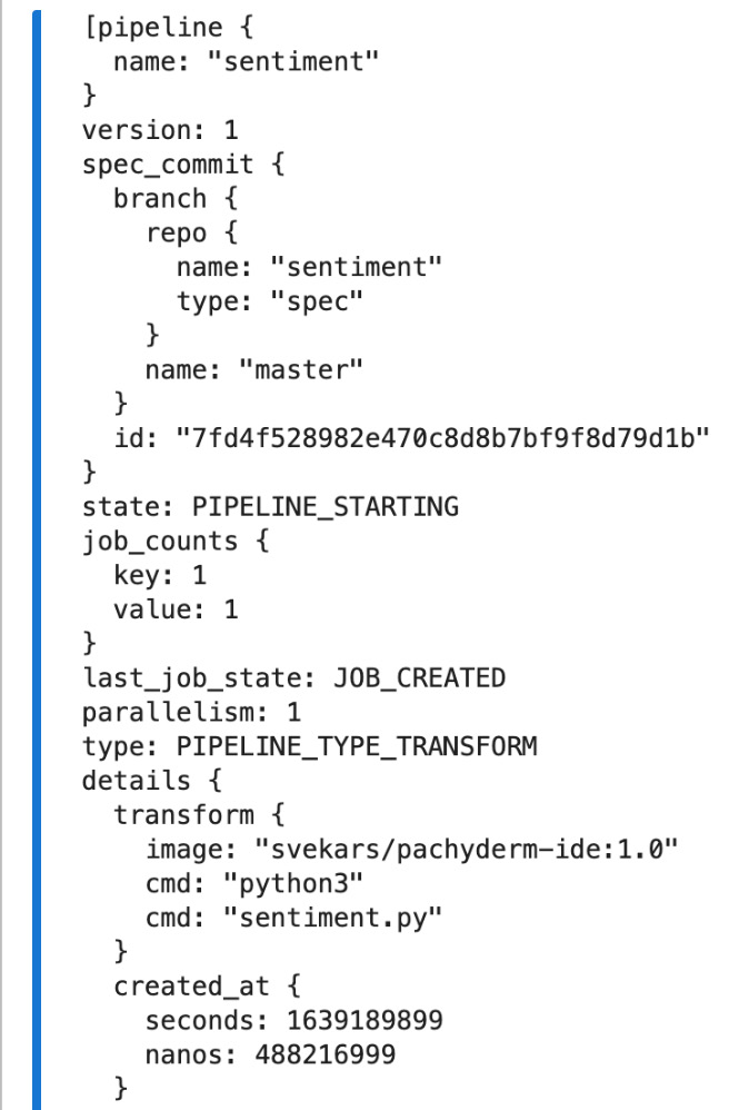
Figure 11.22 – Create pipeline output
The output is truncated and shows only the data-clean pipeline. You should see similar output for the sentiment pipeline.
- Let's view the first few lines of the file in the data-clean repository that has our cleaned data:
import pandas as pd
pd.read_csv(client.get_file(("data-clean", "master"), "cleaned-data.csv"), nrows=10)
This script returns the following output:

Figure 11.23 – Cleaned data
You can see that the text was broken down into tokens.
- Let's get the list of files in the sentiment repository:
list(client.list_file(("sentiment","master"), ""))
You should see a lengthy output. The files will be under path:, similar to the following response:

Figure 11.24 – List of files in the sentiment repository
There should be three files, as follows:
- number_of_tweets.txt: A text file with the total number of tweets in each category
- plot.png: A pie chart with the percentages of tweets in each category
- polarity.csv: A new CSV table with the polarity_score and sentiment columns
- Now, let's look at the first few rows of the polarity.csv table:
pd.read_csv(client.get_file(("sentiment","master"), "polarity.csv"), nrows=10)
This script returns the following output:

Figure 11.25 – Polarity and sentiment results
You can see the two new columns appended to our original table, giving a polarity score in the range [-1;1] and a sentiment category.
- Let's see the total number for each sentiment category:
client.get_file(("sentiment", "master"),"number_of_tweets.txt").read()
You should see the following output:

Figure 11.26 – Total number of tweets for each category
- Finally, let's look at the pie chart with sentiment category percentages:
from IPython.display import display
from PIL import Image
display(Image.open(client.get_file(("sentiment", "master"), "/plot.png")))
This script returns the following output:

Figure 11.27 – Percentage of positive, negative, and neutral sentiments
Based on this chart, we can tell that the majority of the tweets contain positive sentiments and the percentage of negative tweets can be considered insignificant.
This concludes our sentiment analysis example.
Summary
In this chapter, we have learned how to create Pachyderm notebooks in Pachyderm Hub, a powerful addition to Pachyderm that enables data scientists to leverage the benefits of an integrated environment with the Pachyderm data lineage functionality and pipelines. Data scientists spend hours performing exploratory data analysis and do so in notebooks. Combining Pachyderm and notebooks brings data scientists and data engineers together on one platform, letting them speak the same language and use the same tools.
In addition to the above, we created a pipeline that performs basic sentiment analysis of Twitter data and ran it completely in a Pachyderm notebook. We have expanded our knowledge of Python Pachyderm and how it can be used in conjunction with other tools and libraries.
Further reading
- JupyterLab documentation: https://jupyterlab.readthedocs.io/en/stable/
- TextBlob documentation: https://textblob.readthedocs.io/en/dev/
- python-pachyderm documentation: https://python-pachyderm.readthedocs.io/en/stable/