17 Curves and Curved Surfaces

Search in book...
Toggle Font Controls
Create new playlist

Name your new playlist

Playlist description (optional)
Sign In

Email address

Password

Forgot Password?

or

Continue with Facebook

Continue with Google
Sign Up

Full Name

Email address

Confirm Email Address

Password

or

Continue with Facebook

Continue with Google

“Where there is matter, there is geometry.”

—Johannes Kepler

The triangle is a basic atomic rendering primitive. It is what graphics hardware is tuned to rapidly turn into shaded fragments and put into the framebuffer. However, objects and animation paths that are created in modeling systems can have many different underlying geometric descriptions. Curves and curved surfaces can be described precisely by equations. These equations are evaluated and sets of triangles are then created and sent down the pipeline to be rendered.

The beauty of using curves and curved surfaces is at least fourfold: (1) They have a more compact representation than a set of triangles, (2) they provide scalable geometric primitives, (3) they provide smoother and more continuous primitives than straight lines and planar triangles, and (4) animation and collision detection may become simpler and faster.

Compact curve representation offers several advantages for real-time rendering. First, there is savings in memory for model storage (and so some gain in memory cache efficiency). This is especially useful for game consoles, which typically do not have as much memory as a PC. Transforming curved surfaces generally involves fewer matrix multiplications than transforming a mesh representing the surface. If the graphics hardware can accept such curved surface descriptions directly, the amount of data the host CPU has to send to the graphics hardware is usually much less than sending a triangle mesh.

Curved model descriptions such as PN triangles and subdivision surfaces have the worthwhile property that a model with few polygons can be made more convincing and realistic. The individual polygons are treated as curved surfaces, so creating more vertices on the surface. The result of a higher vertex density is better lighting of the surface and silhouette edges with higher quality. See Figure 17.1 for an example.

Figure 17.1. A scene from Call of Duty: Advanced Warfare, where the character Ilona’s face was rendered using Catmull-Clark subdivision surfaces with the adaptive quadtree algorithm from Section 17.6.3. (Image from “Call of Duty,” courtesy of Activision Publishing, Inc. 2018.)

Another major advantage of curved surfaces is that they are scalable. A curved surface description could be turned into 2 triangles or 2000. Curved surfaces are a natural form of on the fly level of detail modeling: When the curved object is close, sample the analytical representation more densely and generate more triangles.

For animation, curved surfaces have the advantage that a much smaller number of points needs to be animated. These points can be used to form a curved surface, and a smooth tessellation can then be generated. Also, collision detection can potentially be more efficient and accurate [939,940].

The topic of curves and curved surfaces has been the subject of entire books [458,777,1242,1504,1847]. Our goal here is to cover curves and surfaces that find common use in real-time rendering.

17.1 Parametric Curves

In this section we will introduce parametric curves. These are used in many different contexts and are implemented using a great many different methods. For real-time graphics, parametric curves are often used to move the viewer or some object along a predefined path. This may involve changing both the position and the orientation. However, in this chapter, we consider only positional paths. See Section for information on orientation interpolation. Another use is to render hair, as seen in Figure 17.2.

Figure 17.2. Hair rendering using tessellated cubic curves [1274]. (Image from “Nalu” demo, courtesy of NVIDIA Corporation.)

Say you want to move the camera from one point to another in a certain amount of time, independent of the performance of the underlying hardware. As an example, assume that the camera should move between these points in one second, and that the rendering of one frame takes 50 ms. This means that we will be able to render 20 frames along the way during that second. On a faster computer, one frame might take only 25 ms, which would be equal to 40 frames per second, and so we would want to move the camera to 40 different locations. Finding either set of points is possible to do with parametric curves.

A parametric curve describes points using some formula as a function of a parameter t. Mathematically, we write this as p(t) $p (t)$ , which means that this function delivers a point for each value of t. The parameter t may belong to some interval, called the domain, e.g., t∈[a,b] $t \in [a, b]$ . The generated points are continuous, that is, as ϵ→0 $ϵ \to 0$ then p(t+ϵ)→p(t) $p (t + ϵ) \to p (t)$ . Loosely speaking, this means that if ϵ $ϵ$ is a minuscule number, then p(t) $p (t)$ and p(t+ϵ) $p (t + ϵ)$ are two points that are extremely close to each other.

In the next section, we will start with an intuitive and geometrical description of Bézier curves, a common form of parametric curves, and then put this into a mathematical setting. Then we discuss how to use piecewise Bézier curves and explain the concept of continuity for curves. In Section 17.1.4 and 17.1.5, we will present two other useful curves, namely cubic Hermites and Kochanek-Bartels splines. Finally, we cover rendering of Bézier curves using the GPU in Section 17.1.2.

17.1.1. Béezier Curves

Linear interpolation traces out a path, which is a straight line, between two points, p0 $p_{0}$ and p1 $p_{1}$ . This is as simple as it gets. See the left illustration in Figure 17.3. Given these points, the following function describes a linearly interpolated point p(t) $p (t)$ , where t is the curve parameter, and t∈[0,1] $t \in [0, 1]$ :

(17.1)

p (t) = p 0 + t (p 1 - p 0) = (1 - t) p 0 + t p 1 .

$\begin{matrix} p (t) = p_{0} + t (p_{1} - p_{0}) = (1 - t) p_{0} + t p_{1} . \end{matrix}$

The parameter t controls where on the line the point p(t) $p (t)$ will land; p(0)=p0 $p (0) = p_{0}$ , p(1)=p1 $p (1) = p_{1}$ , and 0<t<1 $0 < t < 1$ gives us a point on the straight line between p0 $p_{0}$ and p1 $p_{1}$ . So, if we would like to move the camera from p0 $p_{0}$ to p1 $p_{1}$ linearly in 20 steps during one second, then we would use ti=i/(20−1) $t_{i} = i / (20 - 1)$ , where i is the frame number (starting from 0 and ending at 19).

When you are interpolating between only two points, linear interpolation may suffice, but for more points on a path, it often does not. For example, when several points are interpolated, the sudden changes at the points (also called joints) that connect two segments become unacceptable. This is shown at the right of Figure 17.3.

Figure 17.3. Linear interpolation between two points is the path on a straight line (left). For seven points, linear interpolation is shown at the upper right, and some sort of smoother interpolation is shown at the lower right. What is most objectionable about using linear interpolation are the discontinuous changes (sudden jerks) at the joints between the linear segments.

To solve this, we take the approach of linear interpolation one step further, and linearly interpolate repeatedly. By doing this, we arrive at the geometrical construction of the Bézier (pronounced beh-zee-eh) curve. As a historical note, the Bézier curves were developed independently by Paul de Casteljau and Pierre Bézier for use in the French car industry. They are called Bézier curves because Bézier was able to make his research publicly available before de Casteljau, even though de Casteljau wrote his technical report before Bézier [458].

Figure 17.4. Repeated linear interpolation gives a Bézier curve. This curve is defined by three control points, a $a$ , b $b$ , and c $c$ . Assuming we want to find the point on the curve for the parameter t=1/3 $t = 1 / 3$ , we first linearly interpolate between a $a$ and b $b$ to get d $d$ . Next, e $e$ is interpolated from b $b$ and c $c$ . The final point, p(1/3)=f $p (1 / 3) = f$ is found by interpolating between d $d$ and e $e$ .

First, to be able to repeat the interpolation, we have to add more points. For example, three points, a $a$ , b $b$ , and c $c$ , called the control points, could be used. Say we want to find p(1/3) $p (1 / 3)$ , that is, the point on the curve for t=1/3 $t = 1 / 3$ . We compute two new points d $d$ and e $e$ by linear interpolation from a $a$ & b $b$ and b $b$ & c $c$ using t=1/3 $t = 1 / 3$ . See Figure 17.4. Finally, we compute f $f$ by linear interpolation from d $d$ and e $e$ again using t=1/3 $t = 1 / 3$ . We define p(t)=f $p (t) = f$ . Using this technique, we get the following relationship:

(17.2)

p (t) = (1 - t) d + t e = (1 - t) [(1 - t) a + t b] + t [(1 - t) b + t c] = (1 - t) 2 a + 2 (1 - t) t b + t 2 c,

$\begin{matrix} \begin{matrix} p (t) & = (1 - t) d + t e \\ = (1 - t) [(1 - t) a + t b] + t [(1 - t) b + t c] \\ = {(1 - t)}^{2} a + 2 (1 - t) t b + t^{2} c, \end{matrix} \end{matrix}$

which is a parabola since the maximum degree of t is two. In fact, given n+1 $n + 1$ control points, it turns out that the degree of the curve is n. This means that more control points gives more degrees of freedom for the curve. A first degree curve is a straight line (called linear), a second degree curve is called a quadratic, a third degree curve is called a cubic, a fourth degree curve is called a quartic, and so on.

Figure 17.5. Repeated linear interpolation from five points gives a fourth degree (quartic) Bézier curve. The curve is inside the convex hull (green region) of the control points, marked by black dots. Also, at the first point, the curve is tangent to the line between the first and second point. The same also holds for the other end of the curve.

This kind of repeated or recursive linear interpolation is often referred to as the de Casteljau algorithm [458,777]. An example of what this looks like when using five control points is shown in Figure 17.5. To generalize, instead of using points a $a$ – f $f$ , as in this example, the following notation is used. The control points are denoted pi $p_{i}$ , so in the example, p0=a $p_{0} = a$ , p1=b $p_{1} = b$ , and p2=c $p_{2} = c$ . Then, after linear interpolation has been applied k times, intermediate control points pki $p_{i}^{k}$ are obtained. In our example, we have p10=d $p_{0}^{1} = d$ , p11=e $p_{1}^{1} = e$ , and p20=f $p_{0}^{2} = f$ . The Bézier curve for n+1 $n + 1$ control points can be described with the recursion formula shown below, where p0i=pi $p_{i}^{0} = p_{i}$ are the initial control points:

(17.3)

p k i (t) = (1 - t) p k - 1 i (t) + t p k - 1 i + 1 (t), {k i = 1 \dots n, = 0 \dots n - k .

$\begin{matrix} p_{i}^{k} (t) = (1 - t) p_{i}^{k - 1} (t) + t p_{i + 1}^{k - 1} (t), \{\begin{matrix} k & = 1 \dots n, \\ i & = 0 \dots n - k . \end{matrix} \end{matrix}$

Figure 17.6. An illustration of how repeated linear interpolation works for Bézier curves. In this example, the interpolation of a quartic curve is shown. This means there are five control points, p0i $p_{i}^{0}$ , i=0,1,2,3,4 $i = 0, 1, 2, 3, 4$ , shown at the bottom. The diagram should be read from the bottom up, that is, p10 $p_{0}^{1}$ is formed from weighting p00 $p_{0}^{0}$ with weight 1−t $1 - t$ and adding that with p01 $p_{1}^{0}$ weighted by t. This goes on until the point of the curve p(t) $p (t)$ is obtained at the top. (Illustration after Goldman [551].)

Note that a point on the curve is described by p(t)=pn0(t) $p (t) = p_{0}^{n} (t)$ . This is not as complicated as it looks. Consider again what happens when we construct a Bézier curve from three points, p0 $p_{0}$ , p1 $p_{1}$ , and p2 $p_{2}$ , which are equivalent to p00 $p_{0}^{0}$ , p01 $p_{1}^{0}$ , and p02 $p_{2}^{0}$ . Three controls points means that n=2 $n = 2$ . To shorten the formulae, sometimes “(t)” is dropped from the p $p$ ’s. In the first step k=1 $k = 1$ , which gives p10=(1−t)p0+tp1 $p_{0}^{1} = (1 - t) p_{0} + t p_{1}$ , and p11=(1−t)p1+tp2 $p_{1}^{1} = (1 - t) p_{1} + t p_{2}$ . Finally, for k=2 $k = 2$ , we get p20=(1−t)p10+tp11 $p_{0}^{2} = (1 - t) p_{0}^{1} + t p_{1}^{1}$ , which is the same as sought for p(t) $p (t)$ . An illustration of how this works in general is shown in Figure 17.6.

Now that we have the basics in place on how Bézier curves work, we can take a look at a more mathematical description of the same curves.

Béezier Curves Using Bernstein Polynomials

As seen in Equation 17.2, the quadratic Bézier curve could be described using an algebraic formula. It turns out that every Bézier curve can be described with such an algebraic formula, which means that you do not need to do the repeated interpolation. This is shown below in Equation 17.4, which yields the same curve as described by Equation 17.3. This description of the Bézier curve is called the Bernstein form:

(17.4)

p (t) = \sum n i = 0 B n i (t) p i .

$\begin{matrix} p (t) = \sum_{i = 0}^{n} B_{i}^{n} (t) p_{i} . \end{matrix}$

This function contains the Bernstein polynomials, also sometimes called Bézier basis functions,

(17.5)

B n i (t) = (n i) t i (1 - t) n - i = n ! i ! ( n - i ) ! t i (1 - t) n - i .

$\begin{matrix} B_{i}^{n} (t) = (\begin{matrix} n \\ i \end{matrix}) t^{i} {(1 - t)}^{n - i} = \frac{n!}{i! (n - i)!} t^{i} {(1 - t)}^{n - i} . \end{matrix}$

The first term, the binomial coefficient, in this equation is defined in Equation in Chapter 1. Two basic properties of the Bernstein polynomial are the following:

(17.6)

B n i (t) \in [0, 1], when t \in [0, 1], a n d \sum n i = 0 B n i (t) = 1 .

$\begin{matrix} B_{i}^{n} (t) \in [0, 1], when t \in [0, 1], a n d \sum_{i = 0}^{n} B_{i}^{n} (t) = 1 . \end{matrix}$

The first formula means that the Bernstein polynomials are in the interval between 0 to 1 when t also is from 0 to 1. The second formula means that all the Bernstein polynomial terms in Equation 17.4 sum to one for all different degrees of the curve (this can be seen in Figure 17.7). Loosely speaking, this means that the curve will stay “close” to the control points, pi $p_{i}$ . In fact, the entire Bézier curve will be located in the convex hull (see our online linear algebra appendix) of the control points, which follows from Equations 17.4 and 17.6. This is a useful property when computing a bounding area or volume for the curve. See Figure 17.5 for an example.

Figure 17.7. Bernstein polynomials for n=1 $n = 1$ , n=2 $n = 2$ , and n=3 $n = 3$ (left to right). The left figure shows linear interpolation, the middle quadratic interpolation, and the right cubic interpolation. These are the blending functions used in the Bernstein form of Bézier curves. So, to evaluate a quadratic curve (middle diagram) at a certain t-value, just find the t-value on the x-axis, and then go vertically until the three curves are encountered, which gives the weights for the three control points. Note that Bni(t)≥0 $B_{i}^{n} (t) \geq 0$ , when t∈[0,1] $t \in [0, 1]$ , and the symmetry of these blending functions: Bni(t)=Bnn−i(1−t) $B_{i}^{n} (t) = B_{n - i}^{n} (1 - t)$ .

In Figure 17.7 the Bernstein polynomials for n=1 $n = 1$ , n=2 $n = 2$ , and n=3 $n = 3$ are shown. These are also called blending functions. The case when n=1 $n = 1$ (linear interpolation) is illustrative, in the sense that it shows the curves y=1−t $y = 1 - t$ and y=t $y = t$ . This implies that when t=0 $t = 0$ , then p(0)=p0 $p (0) = p_{0}$ , and when t increases, the blending weight for p0 $p_{0}$ decreases, while the blending weight for p1 $p_{1}$ increases by the same amount, keeping the sum of the weights equal to 1. Finally, when t=1 $t = 1$ , p(1)=p1 $p (1) = p_{1}$ . In general, it holds for all Bézier curves that p(0)=p0 $p (0) = p_{0}$ and p(1)=pn $p (1) = p_{n}$ , that is, the endpoints are interpolated (i.e., are on the curve). It is also true that the curve is tangent to the vector p1−p0 $p_{1} - p_{0}$ at t=0 $t = 0$ , and to pn−pn−1 $p_{n} - p_{n - 1}$ at t=1 $t = 1$ . Another useful property is that instead of computing points on a Bézier curve, and then rotating the curve, the control points can first be rotated, and then the points on the curve can be computed. There are usually fewer control points than generated points on the curve, so it is more efficient to transform the control points first.

As an example on how the Bernstein version of the Bézier curve works, assume that n=2 $n = 2$ , i.e., a quadratic curve. Equation 17.4 is then

(17.7)

p (t) [4 p t] [4 p t] = B 20 p 0 + B 21 p 1 + B 22 p 2 = (20) t 0 (1 - t) 2 p 0 + (21) t 1 (1 - t) 1 p 1 + (22) t 2 (1 - t) 0 p 2 = (1 - t) 2 p 0 + 2 t (1 - t) p 1 + t 2 p 2,

$\begin{matrix} \begin{matrix} p (t) & = B_{0}^{2} p_{0} + B_{1}^{2} p_{1} + B_{2}^{2} p_{2} \\ [4 p t] & = (\begin{matrix} 2 \\ 0 \end{matrix}) t^{0} {(1 - t)}^{2} p_{0} + (\begin{matrix} 2 \\ 1 \end{matrix}) t^{1} {(1 - t)}^{1} p_{1} + (\begin{matrix} 2 \\ 2 \end{matrix}) t^{2} {(1 - t)}^{0} p_{2} \\ [4 p t] & = {(1 - t)}^{2} p_{0} + 2 t (1 - t) p_{1} + t^{2} p_{2}, \end{matrix} \end{matrix}$

which is the same as Equation 17.2. Note

that the blending functions above, (1−t)2 ${(1 - t)}^{2}$ , 2t(1−t) $2 t (1 - t)$ , and t2 $t^{2}$ , are the functions displayed in the middle of Figure 17.7. In the same manner, a cubic curve is simplified into

(17.8)

p (t) = (1 - t) 3 p 0 + 3 t (1 - t) 2 p 1 + 3 t 2 (1 - t) p 2 + t 3 p 3 .

$\begin{matrix} p (t) = {(1 - t)}^{3} p_{0} + 3 t {(1 - t)}^{2} p_{1} + 3 t^{2} (1 - t) p_{2} + t^{3} p_{3} . \end{matrix}$

This equation can be rewritten in matrix form as

(17.9)

p (t) = (1 t t 2 t 3) ⎛ ⎝ ⎜ ⎜ ⎜ 1 - 3 3 - 1 03 - 6 3 003 - 3 0001 ⎞ ⎠ ⎟ ⎟ ⎟ ⎛ ⎝ ⎜ ⎜ ⎜ p 0 p 1 p 2 p 3 ⎞ ⎠ ⎟ ⎟ ⎟,

$\begin{matrix} p (t) = (\begin{matrix} 1 & t & t^{2} & t^{3} \end{matrix}) (\begin{matrix} 1 & 0 & 0 & 0 \\ - 3 & 3 & 0 & 0 \\ 3 & - 6 & 3 & 0 \\ - 1 & 3 & - 3 & 1 \end{matrix}) (\begin{matrix} p_{0} \\ p_{1} \\ p_{2} \\ p_{3} \end{matrix}), \end{matrix}$

which is sometimes useful when doing mathematical simplifications.

By collecting terms of the form tk $t^{k}$ in Equation 17.4, it can be seen that every Bézier curve can be written in the following form, called the power form, where the ci $c_{i}$ are points that fall out by collecting terms:

(17.10)

p (t) = \sum n i = 0 t i c i .

$\begin{matrix} p (t) = \sum_{i = 0}^{n} t^{i} c_{i} . \end{matrix}$

It is straightforward to differentiate Equation 17.4, in order to get the derivative of the Bézier curve. The result, after reorganizing and collecting terms, is shown below [458]:

(17.11)

d d t p (t) = n \sum n - 1 i = 0 B n - 1 i (t) (p i + 1 - p i) .

$\begin{matrix} \frac{d}{dt} p (t) = n \sum_{i = 0}^{n - 1} B_{i}^{n - 1} (t) (p_{i + 1} - p_{i}) . \end{matrix}$

The derivative is, in fact, also a Bézier curve, but with one degree lower than p(t) $p (t)$ .

A potential downside of Bézier curves is that they do not pass through all the control points (except the endpoints). Another problem is that the degree increases with the number of control points, making evaluation more and more expensive. A solution to this is to use a simple, low degree curve between each pair of subsequent control points, and see to it that this kind of piecewise interpolation has a high enough degree of continuity. This is the topic of Sections 17.1.3–17.1.5.

Rational Béezier Curves

While Bézier curves can be used for many things, they do not have that many degrees of freedom—only the position of the control points can be chosen freely. Also, not every curve can be described by Bézier curves. For example, the circle is normally considered a simple shape, but it cannot be defined by one or a collection of Bézier curves. One alternative is the rational Bézier curve. This type of curve is described by the formula shown in Equation 17.12:

(17.12)

p (t) = \sum n i = 0 w i B n i ( t ) p i \sum n i = 0 w i B n i ( t ) .

$\begin{matrix} p (t) = \frac{\sum_{i = 0}^{n} w_{i} B_{i}^{n} (t) p_{i}}{\sum_{i = 0}^{n} w_{i} B_{i}^{n} (t)} . \end{matrix}$

The denominator is a weighted sum of the Bernstein polynomials, while the numerator is a weighted version of the standard Bézier curve (Equation 17.4). For this type of curve, the user has the weights, wi $w_{i}$ , as additional degrees of freedom. More about these curves can be found in Hoschek and Lasser’s [777] and in Farin’s book [458]. Farin also describes how a circle can be described by three rational Bézier curves.

17.1.2. Bounded Béezier Curves on the GPU

A method for rendering Bézier curves on the GPU will be presented [1068,1069]. Specifically, the target is “bounded Bézier curves,” where the region between the curve and the straight line between the first and last control points is filled. There is a surprisingly simple way to do this by rendering a triangle with a specialized pixel shader.

Figure 17.8. Bounded Bézier curve rendering. Left: the curve is shown in canonical texture space. Right: the curve is rendered in screen space. If the condition f(u,v)≥0 $f (u, v) \geq 0$ is used to kill pixels, then the light blue region will result from the rendering.

We use a quadratic, i.e., degree two, Bézier curve, with control points p0 $p_{0}$ , p1 $p_{1}$ , and p2 $p_{2}$ . If we set the texture coordinates at these vertices to t0=(0,0) $t_{0} = (0, 0)$ , t1=(0.5,0) $t_{1} = (0.5, 0)$ , and t2=(1,1) $t_{2} = (1, 1)$ , the texture coordinates will be interpolated as usual during rendering of the triangle Δp0p1p2 $Δ p_{0} p_{1} p_{2}$ . We also evaluate the following scalar function inside the triangle for each pixel, where u and v are interpolated texture coordinates:

(17.13)

f (u, v) = u 2 - v .

$\begin{matrix} f (u, v) = u^{2} - v . \end{matrix}$

The pixel shader then determines whether the pixel is inside ( f(u,v)<0 $f (u, v) < 0$ ), or otherwise outside. This is illustrated in Figure 17.8. When rendering a perspective-projected triangle with this pixel shader, we will get the corresponding projected Bézier curve. A proof of this is given by Loop and Blinn [1068,1069].

This type of technique can be used to render TrueType fonts, for example. This is illustrated in Figure 17.9.

Figure 17.9. An e is represented by several straight lines and quadratic Bézier curves (left). In the middle, this representation has been “tessellated” into several bounded Bézier curves (red and blue), and triangles (green). The final letter is shown to the right. (Reprinted with permission from Microsoft Corporation.)

Loop and Blinn also show how to render rational quadratic curves and cubic curves, and how do to antialiasing using this representation. Because of the importance of text rendering, research in this area has continued. See Section for related algorithms.

17.1.3. Continuity and Piecewise Béezier Curves

Assume that we have two Bézier curves that are cubic, that is, defined by four control points each. The first curve is defined by $q_{i}$ , and the second by $r_{i}$ , $i = 0, 1, 2, 3$ . To join the curves, we could set $q_{3} = r_{0}$ . This point is called a joint. However, as shown in Figure 17.10, the joint will not be smooth using this simple technique.

Figure 17.10. This figure shows from left to right $C^{0}$ , $G^{1}$ , and $C^{1}$ continuity between two cubic Bézier curves (four control points each). The top row shows the control points, and the bottom row the curves, with 10 sample points for the left curve, and 20 for the right. The following time-point pairs are used for this example: $(0.0, q_{0})$ , $(1.0, q_{3})$ , and $(3.0, r_{3})$ . With $C^{0}$ continuity, there is a sudden jerk at the join (where $q^{3} = r^{0}$ ). This is improved with $G^{1}$ by making the tangents at the join parallel (and equal in length). Though, since $3.0 - 1.0 \neq 1.0 - 0.0$ , this does not give $C^{1}$ continuity. This can be seen at the join where there is a sudden acceleration of the sample points. To achieve $C^{1}$ , the right tangent at the join has to be twice as long as the left tangent.

The composite curve formed from several curve pieces (in this case two) is called a piecewise Bézier curve, and is denoted $p (t)$ here. Further, assume we want $p (0) = q_{0}$ , $p (1) = q_{3} = r_{0}$ , and $p (3) = r_{3}$ . Thus, the times for when we reach $q_{0}$ , $q_{3} = r_{0}$ , and $r_{3}$ , are $t_{0} = 0.0$ , $t_{1} = 1.0$ , and $t_{2} = 3.0$ . See Figure 17.10 for notation. From the previous section we know that a Bézier curve is defined for $t \in [0, 1]$ , so this works out fine for the first curve segment defined by the $q_{i}$ ’s, since the time at $q_{0}$ is 0.0, and the time at $q_{3}$ is 1.0. But what happens when $1.0 < t \leq 3.0$ ? The answer is simple: We must use the second curve segment, and then translate and scale the parameter interval from $[t_{1}, t_{2}]$ to [0, 1]. This is done using the formula below:

(17.14)

$\begin{matrix} t^{'} = \frac{t - t_{1}}{t_{2} - t_{1}} . \end{matrix}$

Hence, it is the $t^{'}$ that is fed into the Bézier curve segment defined by the $r_{i}$ ’s. This is simple to generalize to stitching several Bézier curves together.

A better way to join the curves is to use the fact that at the first control point of a Bézier curve the tangent is parallel to $q_{1} - q_{0}$ (Section 17.1.1). Similarly, at the last control point the cubic curve is tangent to $q_{3} - q_{2}$ . This behavior can be seen in Figure 17.5. So, to make the two curves join tangentially at the joint, the tangent for the first and the second curve should be parallel there. Put more formally, the following should hold:

(17.15)

$\begin{matrix} \begin{matrix} (r_{1} - r_{0}) = c (q_{3} - q_{2}) & for c > 0 . \end{matrix} \end{matrix}$

This simply means that the incoming tangent, $q_{3} - q_{2}$ , at the joint should have the same direction as the outgoing tangent, $r_{1} - r_{0}$ .

It is possible to achieve even better continuity than that, using in Equation 17.15 the c defined by Equation 17.16 [458]:

(17.16)

$\begin{matrix} c = \frac{t_{2} - t_{1}}{t_{1} - t_{0}} . \end{matrix}$

This is also shown in Figure 17.10. If we instead set $t_{2} = 2.0$ , then $c = 1.0$ , so when the time intervals on each curve segment are equal, then the incoming and outgoing tangent vectors should be identical. However, this does not work when $t_{2} = 3.0$ . The curves will look identical, but the speed at which $p (t)$ moves on the composite curve will not be smooth. The constant c in Equation 17.16 takes care of this.

Some advantages of using piecewise curves are that lower-degree curves can be used, and that the resulting curves will go through a set of points. In the example above, a degree of three, i.e., a cubic, was used for each of the two curve segments. Cubic curves are often used for this, as those are the lowest-degree curves that can describe an S-shaped curve, called an inflection. The resulting curve $p (t)$ interpolates, i.e., goes through, the points $q_{0}$ , $q_{3} = r_{0}$ , and $r_{3}$ .

At this point, two important continuity measures have been introduced by example. A slightly more mathematical presentation of the continuity concept for curves follows. For curves in general, we use the $C^{n}$ notation to differentiate between different kinds of continuity at the joints. This means that all the nth first derivatives should be continuous and nonzero all over the curve. Continuity of $C^{0}$ means that the segment should join at the same point, so linear interpolation fulfills this condition. This was the case for the first example in this section. Continuity of $C^{1}$ means that if we derive once at any point on the curve (including joints), the result should also be continuous. This was the case for the third example in this section, where Equation 17.16was used.

There is also a measure that is denoted $G^{n}$ . Let us look at $G^{1}$ (geometrical) continuity as an example. For this, the tangent vectors from the curve segments that meet at a joint should be parallel and have the same direction, but nothing about the lengths is assumed. In other words, $G^{1}$ is a weaker continuity than $C^{1}$ , and a curve that is $C^{1}$ is always $G^{1}$ except when the velocities of two curves go to zero at the point where the curves join and they have different tangents just before the join. The concept of geometrical continuity can be extended to higher dimensions. The middle illustration in Figure 17.10 shows $G^{1}$ -continuity.

Figure 17.11. Blending functions for Hermite cubic interpolation. Note the asymmetry of the blending functions for the tangents. Negating the blending function $t^{3} - t^{2}$ and $m_{1}$ in Equation 17.17 would give a symmetrical look.

Figure 17.12. Hermite interpolation. A curve is defined by two points, $p_{0}$ and $p_{1}$ , and a tangent, $m_{0}$ and $m_{1}$ , at each point.

17.1.4. Cubic Hermite Interpolation

Bézier curves are good for describing the theory behind the construction of smooth curves, but are sometimes not predictable to work with.

In this section, we will present cubic Hermite interpolation, and these curves tend to be simpler to control. The reason is that instead of giving four control points to describe a cubic Bézier curve, the cubic Hermite curve is defined by starting and ending points, $p_{0}$ and $p_{1}$ , and starting and ending tangents, $m_{0}$ and $m_{1}$ . The Hermite interpolant, $p (t)$ , where $t \in [0, 1]$ , is

(17.17)

$\begin{matrix} p (t) = (2 t^{3} - 3 t^{2} + 1) p_{0} + (t^{3} - 2 t^{2} + t) m_{0} + (t^{3} - t^{2}) m_{1} + (- 2 t^{3} + 3 t^{2}) p_{1} . \end{matrix}$

We also call $p (t)$ a Hermite curve segment or a cubic spline segment. This is a cubic interpolant, since $t^{3}$ is the highest exponent in the blending functions in the above formula. The following holds for this curve:

(17.18)

$\begin{matrix} p (0) = p_{0}, p (1) = p_{1}, \frac{\partial p}{\partial t} (0) = m_{0}, \frac{\partial p}{\partial t} (1) = m_{1} . \end{matrix}$

This means that the Hermite curve interpolates $p_{0}$ and $p_{1}$ , and the tangents at these points are $m_{0}$ and $m_{1}$ . The blending functions in Equation 17.17 are shown in Figure 17.11, and they can be derived from Equations 17.4 and 17.18. Some examples of cubic Hermite interpolation can be seen in Figure 17.12. All these examples interpolate the same points, but have different tangents. Note also that different lengths of the tangents give different results; longer tangents have a greater impact on the overall shape.

Cubic Hermite interpolation is used to render the hair in the Nalu demo [1274]. See Figure 17.2. A coarse control hair is used for animation and collision detection, tangents are computed, and cubic curves are tessellated and rendered.

17.1.5. Kochanek-Bartels Curves

When interpolating between more than two points, you can connect several Hermite curves.

However, when doing this, there are degrees of freedom in selecting the shared tangents that provide different characteristics. Here, we will present one way to compute such tangents, called Kochanek-Bartels curves. Assume that we have n points, $p_{0}, \dots, p_{n - 1}$ , which should be interpolated with $n - 1$ Hermite curve segments. We assume that there is only one tangent at each point, and we start to look at the “inner” tangents, $m_{1}, \dots, m_{n - 2}$ . A tangent at $p_{i}$ can be computed as a combination of the two chords [917]: $p_{i} - p_{i - 1}$ , and $p_{i + 1} - p_{i}$ , as shown at the left in Figure 17.13.

Figure 17.13. One method of computing the tangents is to use a combination of the chords (left). The upper row at the right shows three curves with different tension parameters (a). The left curve has $a \approx 1$ , which means high tension; the middle curve has $a \approx 0$ , which is default tension; and the right curve has $a \approx - 1$ , which is low tension. The bottom row of two curves at the right shows different bias parameters. The curve on the left has a negative bias, and the right curve has a positive bias.

First, a tension parameter, a, is introduced that modifies the length of the tangent vector. This controls how sharp the curve is going to be at the joint. The tangent is computed as

(17.19)

$\begin{matrix} m_{i} = \frac{1 - a}{2} ((p_{i} - p_{i - 1}) + (p_{i + 1} - p_{i})) . \end{matrix}$

The top row at the right in Figure 17.13 shows different tension parameters. The default value is $a = 0$ ; higher values give sharper bends (if $a > 1$ , there will be a loop at the joint), and negative values give less taut curves near the joints. Second, a bias parameter, b, is introduced that influences the direction of the tangent (and, indirectly, the length of the tangent).

Using both tension and bias gives us

(17.20)

$\begin{matrix} m_{i} = \frac{(1 - a) (1 + b)}{2} (p_{i} - p_{i - 1}) + \frac{(1 - a) (1 - b)}{2} (p_{i + 1} - p_{i}), \end{matrix}$

where the default value is $b = 0$ . A positive bias gives a bend that is more directed toward the chord $p_{i} - p_{i - 1}$ , and a negative bias gives a bend that is more directed toward the other chord: $p_{i + 1} - p_{i}$ . This is shown in the bottom row on the right in Figure 17.13. The user can either set the tension and bias parameters or let

them have their default values, which produces what is often called a Catmull-Rom spline [236]. The tangents at the first and the last points can also be computed with these formulae, where one of the chords is simply set to a length of zero.

Yet another parameter that controls the behavior at the joints can be incorporated into the tangent equation [917]. However, this requires the introduction of two tangents at each joint, one incoming, denoted $s_{i}$ (for source) and one outgoing, denoted $d_{i}$ (for destination). See Figure 17.14. Note that the curve segment between $p_{i}$ and $p_{i + 1}$ uses the tangents $d_{i}$ and $s_{i + 1}$ . The tangents are computed as below, where c is the continuity parameter:

(17.21)

$\begin{matrix} \begin{matrix} s_{i} = \frac{1 - c}{2} (p_{i} - p_{i - 1}) + \frac{1 + c}{2} (p_{i + 1} - p_{i}), \\ [2 p t] d_{i} = \frac{1 + c}{2} (p_{i} - p_{i - 1}) + \frac{1 - c}{2} (p_{i + 1} - p_{i}) . \end{matrix} \end{matrix}$

Figure 17.14. Incoming and outgoing tangents for Kochanek-Bartels curves. At each control point $p_{i}$ , its time $t_{i}$ is also shown, where $t_{i} > t_{i - 1}$ , for all i.

Again, $c = 0$ is the default value, which makes $s_{i} = d_{i}$ . Setting $c = - 1$ gives $s_{i} = p_{i} - p_{i - 1}$ , and $d_{i} = p_{i + 1} - p_{i}$ , producing a sharp corner at the joint, which is only $C^{0}$ . Increasing the value of c makes $s_{i}$ and $d_{i}$ more and more alike. For $c = 0$ , then $s_{i} = d_{i}$ . When $c = 1$ is reached, we get $s_{i} = p_{i + 1} - p_{i}$ , and $d_{i} = p_{i} - p_{i - 1}$ . Thus, the continuity parameter c is another way to give even more control to the user, and it makes it possible to get sharp corners at the joints, if desired.

The combination of tension, bias, and continuity, where the default parameter values are $a = b = c = 0$ , is

(17.22)

$\begin{matrix} \begin{matrix} s_{i} & = \frac{(1 - a) (1 + b) (1 - c)}{2} (p_{i} - p_{i - 1}) + \frac{(1 - a) (1 - b) (1 + c)}{2} (p_{i + 1} - p_{i}), \\ [2 p t] d_{i} & = \frac{(1 - a) (1 + b) (1 + c)}{2} (p_{i} - p_{i - 1}) + \frac{(1 - a) (1 - b) (1 - c)}{2} (p_{i + 1} - p_{i}) . \end{matrix} \end{matrix}$

Both Equations 17.20 and 17.22 work only when all curve segments are using the same time interval length. To account for different time length of the curve segments, the tangents have to be adjusted, similar to what was done in Section 17.1.3. The adjusted tangents, denoted $s_{i}^{'}$ and $d_{i}^{'}$ , are

(17.23)

$\begin{matrix} s_{i}^{'} = s_{i} \frac{2 Δ_{i}}{Δ_{i - 1} + Δ_{i}} a n d d_{i}^{'} = d_{i} \frac{2 Δ_{i - 1}}{Δ_{i - 1} + Δ_{i}}, \end{matrix}$

where $Δ_{i} = t_{i + 1} - t_{i}$ .

17.1.6. B-Splines

Here, we will provide a brief introduction to the topic of B-splines, and we will focus in particular on cubic uniform B-splines. In general, a B-spline is quite similar to a Bézier curve, and can be expressed as a function of t (using shifted basis functions), $β_{n}$ (weighted by control points), and $c_{k}$ : e.g.,

(17.24)

$\begin{matrix} s_{n} (t) = \sum_{k} c_{k} β_{n} (t - k) . \end{matrix}$

In this case, this is a curve where t is the x-axis and $s_{n} (t)$ is the y-axis, and the control points are simply evenly spaced y-values. For much more extensive coverage, see the texts by the Killer B’s [111], Farin [458], and Hoschek and Lasser [777].

Here, we will follow the presentation by Ruijters et al. [1518] and present the special case of a uniform cubic B-spline. The basis function, $β_{3} (t)$ , is stitched together by three pieces:

(17.25)

$\begin{matrix} β_{3} (t) = \{\begin{matrix} 0, & | t | \geq 2, \\ [2 p t] \frac{1}{6} {(2 - | t |)}^{3}, & 1 \leq | t | < 2, \\ [2 p t] \frac{2}{3} - \frac{1}{2} {| t |}^{2} (2 - | t |), & | t | < 1 . \end{matrix} \end{matrix}$

The construction of this basis function is shown on the left in Figure 17.15. This function has $C^{2}$ continuity everywhere, which means that if several B-spline curve segments are stitched together, the composite curve will also be $C^{2}$ . A cubic curve has $C^{2}$ continuity, and in general, a curve of degree n has $C^{n - 1}$ continuity.

Figure 17.15. Left: the $β_{3} (t)$ basis function is shown as a fat black curve, which is constructed from two piecewise cubic functions (red and green). The green curve is used when $| t | < 1$ , the red curve when $1 \leq | t | < 2$ , and the curve is zero elsewhere. Right: to create a curve segment using four control points, $c_{k}$ , $k \in {i - 1, i, i + 1, i + 2}$ , we will only obtain a curve between the t-coordinate of $c_{i}$ and of $c_{i} + 1$ . The $α$ is fed into the w functions to evaluate the basis function, and these values are then multiplied by the corresponding control point. Finally, all values are added together, which gives us a point on the curve. See Figure 17.16. (Illustration on the right after Ruijters et al. [1518].)

In general, the basis functions are created as follows. The $β_{0} (t)$ is a “square” function, i.e., it is 1 if $| t | < 0.5$ , it is 0.5 if $| t | = 0.5$ , and it is 0 elsewhere. The next basis function, $β_{1} (t)$ is created by integrating $β_{0} (t)$ , which gives us a tent function. The basis function after that is created by integrating $β_{1} (t)$ , which gives a smoother function, which is $C^{1}$ . This process is repeated to get $C^{2}$ , and so on.

How to evaluate a curve segment is illustrated on the right in Figure 17.15, and its formula is

(17.26)

$\begin{matrix} s_{3} (i + α) = w_{0} (α) c_{i - 1} + w_{1} (α) c_{i} + w_{2} (α) c_{i + 1} + w_{3} (α) c_{i + 2} . \end{matrix}$

Note that only four control points will be used at any time, and this means that the curve has local support, i.e., a limited number of control points is needed. The functions $w_{k} (α)$ are defined using $β_{3} ()$ as

(17.27)

$\begin{matrix} \begin{matrix} w_{0} (α) = β_{3} (- α - 1), & w_{1} (α) = β_{3} (- α), \\ w_{2} (α) = β_{3} (1 - α), & w_{3} (α) = β_{3} (2 - α) . \end{matrix} \end{matrix}$

Ruijters et al. [1518] show that these can be rewritten as

(17.28)

$\begin{matrix} \begin{matrix} w_{0} (α) = \frac{1}{6} {(1 - α)}^{3}, & w_{1} (α) = \frac{2}{3} - \frac{1}{2} α^{2} (2 - α), \\ w_{2} (α) = \frac{2}{3} - \frac{1}{2} {(1 - α)}^{2} (1 + α), & w_{3} (α) = \frac{1}{6} α^{3} . \end{matrix} \end{matrix}$

In Figure 17.16, we show the results of stitching two uniform cubic B-spline curves together as one.

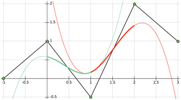
Figure 17.16. The control points $c_{k}$ (green circles) define a uniform cubic spline in this example. Only the two fat curves are part of the piecewise B-spline curve. The left (green) curve is defined by the four leftmost control points, and the right (red) curve is defined by the four rightmost control points. The curves meet at $t = 1$ with $C^{2}$ continuity.

A major advantage is that the curves are continuous with the same continuity as the basis functions, $β (t)$ , which are $C^{2}$ in the case of a cubic B-spline. As can be seen in the figure, there is no guarantee that the curve will go through any of the control points. Note that we can also create a B-spline for the x-coordinates, which would give a general curve in the plane (and not just a function). The resulting two-dimensional points would then be $(s_{3}^{x} (i + α), s_{3}^{y} (i + α))$ , i.e., simply two different evaluations of Equation 17.26, one for x and one for y.

We have shown how to use only B-splines that are uniform. If the spacing between the control points is nonuniform, the equations become a bit more elaborate but more flexible [111,458,777].

17.2 Parametric Curved Surfaces

A natural extension of parametric curves is parametric surfaces. An analogy is that a triangle or polygon is an extension of a line segment, in which we go from one to two dimensions. Parametric surfaces can be used to model objects with curved surfaces. A parametric surface is defined by a small number of control points. Tessellation of a parametric surface is the process of evaluating the surface representation at several positions, and connecting these to form triangles that approximate the true surface. This is done because graphics hardware can efficiently render triangles. At runtime, the surface can then be tessellated into as many triangles as desired. Thus, parametric surfaces are perfect for making a trade-off between quality and speed, since more triangles take more time to render, but give better shading and silhouettes. Another advantage of parametric surfaces is that the control points can be animated and then the surface can be tessellated. This is in contrast to animating a large triangle mesh directly, which can be more expensive.

This section starts by introducing Bézier patches, which are curved surfaces with rectangular domains. These are also called tensor-product Bézier surfaces. Then Bézier triangles are presented, which have triangular domains, followed by a discussion about continuity in Section 17.2.4. In Sections 17.2.5 and 17.2.6, two methods are presented that replace each input triangle with a Bézier triangle. These techniques are called PN triangles and Phong tessellation, respectively. Finally, B-spline patches are presented in Section 17.2.7.

17.2.1. Béezier Patches

The concept of Bézier curves, introduced in Section 17.1.1, can be extended from using one parameter to using two parameters, thus forming surfaces instead of curves. Let us start with extending linear interpolation to bilinear interpolation. Now, instead of just using two points, we use four points, called $a$ , $b$ , $c$ , and $d$ , as shown in Figure 17.17.

Figure 17.17. Bilinear interpolation using four points.

Figure 17.18. Left: a biquadratic Bézier surface, defined by nine control points, $p_{ij}$ . Right: to generate a point on the Bézier surface, four points $p_{ij}^{1}$ are first created using bilinear interpolation from the nearest control points. Finally, the point surface $p (u, v) = p_{00}^{2}$ is bilinearly interpolated from these created points.

Instead of using one parameter called t, we now use two parameters (u, v). Using u to linearly interpolate $a$ & $b$ and $c$ & $d$ gives $e$ and $f$ :

(17.29)

$\begin{matrix} e = (1 - u) a + u b, f = (1 - u) c + u d . \end{matrix}$

Next, the linearly interpolated points, $e$ and $f$ , are linearly interpolated in the other direction, using v. This yields bilinear interpolation:

(17.30)

$\begin{matrix} \begin{matrix} p (u, v) & = (1 - v) e + v f \\ = (1 - u) (1 - v) a + u (1 - v) b + (1 - u) v c + u v d . \end{matrix} \end{matrix}$

Note that this is the same type of equation used for bilinear interpolation for texture mapping (Equation on page 179). Equation 17.30 describes the simplest nonplanar parametric surface, where different points on the surface are generated using different values of (u, v). The domain, i.e., the set of valid values, is $(u, v) \in [0, 1] \times [0, 1]$ , which means that both u and v should belong to [0, 1]. When the domain is rectangular, the resulting surface is often called a patch.

To extend a Bézier curve from linear interpolation, more points were added and the interpolation repeated. The same strategy can be used for patches. Assume nine points, arranged in a $3 \times 3$ grid, are used. This is shown in Figure 17.18, where the notation is shown as well. To form a biquadratic Bézier patch from these points, we first need to bilinearly interpolate four times to create four intermediate points, also shown in Figure 17.18. Next, the final point on the surface is bilinearly interpolated from the previously created points.

The repeated bilinear interpolation described above is the extension of de Casteljau’s algorithm to patches. At this point we need to define some notation. The degree of the surface is n. The control points are $p_{i, j}$ , where i and j belong to $[0 \dots n]$ . Thus, ${(n + 1)}^{2}$ control points are used for a patch of degree n. Note that the control points should be superscripted with a zero, i.e., $p_{i, j}^{0}$ , but this is often omitted, and sometimes we use the subscript $_{ij}$ instead of $_{i, j}$ when there can be no confusion. The Bézier patch using de Casteljau’s algorithm is described in the equation that follows:

de Casteljau [patches]:

(17.31)

$\begin{matrix} \begin{matrix} p_{i, j}^{k} (u, v) & = (1 - u) (1 - v) p_{i, j}^{k - 1} + u (1 - v) p_{i, j + 1}^{k - 1} + (1 - u) v p_{i + 1, j}^{k - 1} + u v p_{i + 1, j + 1}^{k - 1} \\ k & = 1 \dots n, i = 0 \dots n - k, j = 0 \dots n - k . \end{matrix} \end{matrix}$

Similar to the Bézier curve, the point at (u, v) on the Bézier patch is $p_{0, 0}^{n} (u, v)$ . The Bézier patch can also be described in Bernstein form using Bernstein polynomials, as shown in Equation 17.32:

Bernstein [patches]:

(17.32)

$\begin{matrix} \begin{matrix} p (u, v) & = \sum_{i = 0}^{m} B_{i}^{m} (u) \sum_{j = 0}^{n} B_{j}^{n} (v) p_{i, j} = \sum_{i = 0}^{m} \sum_{j = 0}^{n} B_{i}^{m} (u) B_{j}^{n} (v) p_{i, j}, \\ = \sum_{i = 0}^{m} \sum_{j = 0}^{n} (\begin{matrix} m \\ i \end{matrix}) (\begin{matrix} n \\ j \end{matrix}) u^{i} {(1 - u)}^{m - i} v^{j} {(1 - v)}^{n - j} p_{i, j} . \end{matrix} \end{matrix}$

Note that in Equation 17.32, there are two parameters, m and n, for the degree of the surface. The “compound” degree is sometimes denoted $m \times n$ . Most often $m = n$ , which simplifies the implementation a bit. The consequence of, say, $m > n$ is to first bilinearly interpolate n times, and then linearly interpolate $m - n$ times. This is shown in Figure 17.19.

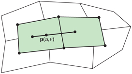
Figure 17.19. Different degrees in different directions.

A different interpretation of Equation 17.32 is found by rewriting it as

(17.33)

$\begin{matrix} p (u, v) = \sum_{i = 0}^{m} B_{i}^{m} (u) \sum_{j = 0}^{n} B_{j}^{n} (v) p_{i, j} \\ [6 p t] = \sum_{i = 0}^{m} B_{i}^{m} (u) q_{i} (v) . \end{matrix}$

Here, $q_{i} (v) = \sum_{j = 0}^{n} B_{j}^{n} (v) p_{i, j}$ for $i = 0 \dots m$ . As can be seen in the bottom row in Equation 17.33, this is just a Bézier curve when we fix a v-value. Assuming $v = 0.35$ , the points $q_{i} (0.35)$ can be computed from a Bézier curve, and then Equation 17.33 describes a Bézier curve on the Bézier surface, for $v = 0.35$ .

Next, some useful properties of Bézier patches will be presented. By setting $(u, v) = (0, 0)$ , $(u, v) = (0, 1)$ , $(u, v) = (1, 0)$ , and $(u, v) = (1, 1)$ in Equation 17.32, it is simple to prove that a Bézier patch interpolates, that is, goes through, the corner control points, $p_{0, 0}$ , $p_{0, n}$ , $p_{n, 0}$ , and $p_{n, n}$ . Also, each boundary of the patch is described by a Bézier curve of degree n formed by the control points on the boundary. Therefore, the tangents at the corner control points are defined by these boundary Bézier curves. Each corner control point has two tangents, one in each of the u- and v-directions. As was the case for Bézier curves, the patch also lies within the convex hull of its control points, and

(17.34)

$\begin{matrix} \sum_{i = 0}^{m} \sum_{j = 0}^{n} B_{i}^{m} (u) B_{j}^{n} (v) = 1 \end{matrix}$

for $(u, v) \in [0, 1] \times [0, 1]$ . Finally, rotating the control points and then generating points on the patch is the same mathematically as (though usually faster than) generating points on the patch and then rotating these.

Partially differentiating Equation 17.32 gives [458] the equations below:

Derivatives [patches]:

(17.35)

$\begin{matrix} \begin{matrix} \frac{\partial p (u, v)}{\partial u} & = m \sum_{j = 0}^{n} \sum_{i = 0}^{m - 1} B_{i}^{m - 1} (u) B_{j}^{n} (v) [p_{i + 1, j} - p_{i, j}], \\ [3 p t] \frac{\partial p (u, v)}{\partial v} & = n \sum_{i = 0}^{m} \sum_{j = 0}^{n - 1} B_{i}^{m} (u) B_{j}^{n - 1} (v) [p_{i, j + 1} - p_{i, j}] . \end{matrix} \end{matrix}$

As can be seen, the degree of the patch is reduced by one in the direction that is differentiated. The unnormalized normal vector is then formed as

(17.36)

$\begin{matrix} n (u, v) = \frac{\partial p (u, v)}{\partial u} \times \frac{\partial p (u, v)}{\partial v} . \end{matrix}$

In Figure 17.20, the control mesh together with the actual Bézier patch is shown. The effect of moving a control point is shown in Figure 17.21.

Rational Béezier Patches

Just as the Bézier curve could be extended into a rational Bézier curve (Section 17.1.1), and thus introduce more degrees of freedom, so can the Bézier patch be extended into a rational Bézier patch:

(17.37)

$\begin{matrix} p (u, v) = \frac{\sum_{i = 0}^{m} \sum_{j = 0}^{n} w_{i, j} B_{i}^{m} (u) B_{j}^{n} (v) p_{i, j}}{\sum_{i = 0}^{m} \sum_{j = 0}^{n} w_{i, j} B_{i}^{m} (u) B_{j}^{n} (v)} . \end{matrix}$

Consult Farin’s book [458] and Hochek and Lasser’s book [777] for information about this type of patch. Similarly, the rational Bézier triangle is an extension of the Bézier triangle, treated next.

Figure 17.20. Left: control mesh of a $4 \times 4$ Bézier patch of degree $3 \times 3$ . Middle: the actual quadrilaterals that were generated on the surface. Right: shaded Bézier patch.

Figure 17.21. This set of images shows what happens to a Bézier patch when one control point is moved. Most of the change is near the moved control point.

Figure 17.22. The control points of a Bézier triangle with degree three (cubic).

17.2.2. Béezier Triangles

Even though the triangle often is considered a simpler geometric primitive than the rectangle, this is not the case when it comes to Bézier surfaces: Bézier triangles are not as straightforward as Bézier patches. This type of patch is worth presenting as it is used in forming PN triangles and for Phong tessellation, which are fast and simple.

Note that some game engines, such as the Unreal Engine, Unity, and Lumberyard, support Phong tessellation and PN triangles.

The control points are located in a triangular grid, as shown in Figure 17.22.

The degree of the Bézier triangle is n, and this implies that there are $n + 1$ control points per side. These control points are denoted $p_{i, j, k}^{0}$ and sometimes abbreviated to $p_{ijk}$ . Note that $i + j + k = n$ , and $i, j, k \geq 0$ for all control points. Thus, the total number of control points is

(17.38)

$\begin{matrix} \sum_{x = 1}^{n + 1} x = \frac{(n + 1) (n + 2)}{2} . \end{matrix}$

It should come as no surprise that Bézier triangles also are based on repeated interpolation. However, due to the triangular shape of the domain, barycentric coordinates (Section ) must be used for the interpolation. Recall that a point within a triangle $Δ p_{0} p_{1} p_{2}$ , can be described as $p (u, v) = p_{0} + u (p_{1} - p_{0}) + v (p_{2} - p_{0}) = (1 - u - v) p_{0} + u p_{1} + v p_{2}$ , where (u, v) are the barycentric coordinates. For points inside the triangle the following must hold: $u \geq 0$ , $v \geq 0$ , and $1 - (u + v) \geq 0 \Leftrightarrow u + v \leq 1$ . Based on this, the de Casteljau algorithm for Bézier triangles is

de Casteljau [triangles]:

(17.39)

$\begin{matrix} \begin{matrix} p_{i, j, k}^{l} (u, v) & = u p_{i + 1, j, k}^{l - 1} + v p_{i, j + 1, k}^{l - 1} + (1 - u - v) p_{i, j, k + 1}^{l - 1}, \\ l & = 1 \dots n, i + j + k = n - l . \end{matrix} \end{matrix}$

The final point on the Bézier triangle at (u, v) is $p_{000}^{n} (u, v)$ . The Bézier triangle in Bernstein form is

(17.40)

$\begin{matrix} Bernstein [triangles] : & p (u, v) & = \sum_{i + j + k = n} B_{ijk}^{n} (u, v) p_{ijk} . \end{matrix}$

The Bernstein polynomials now depend on both u and v, and are therefore computed differently, as shown below:

(17.41)

$\begin{matrix} B_{ijk}^{n} (u, v) = \frac{n!}{i! j! k!} u^{i} v^{j} {(1 - u - v)}^{k}, i + j + k = n . \end{matrix}$

The partial derivatives are [475]

Derivatives [triangles]:

(17.42)

$\begin{matrix} \begin{matrix} \frac{\partial p (u, v)}{\partial u} & = \sum_{i + j + k = n - 1} n B_{ijk}^{n - 1} (u, v) (p_{i + 1, j, k} - p_{i, j, k + 1}), \\ \frac{\partial p (u, v)}{\partial v} & = \sum_{i + j + k = n - 1} n B_{ijk}^{n - 1} (u, v) (p_{i, j + 1, k} - p_{i, j, k + 1}) . \end{matrix} \end{matrix}$

Some unsurprising properties of Bézier triangles are that they interpolate (pass through) the three corner control points, and that each boundary is a Bézier curve described by the control points on that boundary. Also, the surfaces lies in the convex hull of the control points. A Bézier triangle is shown in Figure 17.23.

Figure 17.23. Left: wireframe of a tessellated Bézier triangle. Right: shaded surface together with control points.

17.2.3. Continuity

When constructing a complex object from Bézier surfaces, one often wants to stitch together several different Bézier surfaces to form one composite surface. To get a good-looking result, care must be taken to ensure that reasonable continuity is obtained across the surfaces. This is in the same spirit as for curves, in Section 17.1.3.

Figure 17.24. How to stitch together two Bézier patches with $C^{1}$ continuity. All control points on bold lines must be collinear, and they must have the same ratio between the two segment lengths. Note that $a_{3 j} = b_{0 j}$ to get a shared boundary between patches. This can also be seen to the right in Figure 17.25.

Assume two bicubic Bézier patches should be pieced together. These have $4 \times 4$ control points each. This is illustrated in Figure 17.24, where the left patch has control points, $a_{ij}$ , and the right has control points, $b_{ij}$ , for $0 \leq i, j \leq 3$ . To ensure $C^{0}$ continuity, the patches must share the same control points at the border, that is, $a_{3 j} = b_{0 j}$ .

However, this is not sufficient to get a nice looking composite surface. Instead, a simple technique will be presented that gives $C^{1}$ continuity [458]. To achieve this we must constrain the position of the two rows of control points closest to the shared control points. These rows are $a_{2 j}$ and $b_{1 j}$ . For each j, the points $a_{2 j}$ , $b_{0 j}$ , and $b_{1 j}$ must be collinear, that is, they must lie on a line. Moreover, they must have the same ratio, which means that $| | a_{2 j} - b_{0 j} | | = k | | b_{0 j} - b_{1 j} | |$ . Here, k is a constant, and it must be the same for all j. Examples are shown in Figure 17.24 and 17.25.

This sort of construction uses up many degrees of freedom of setting the control points. This can be seen even more clearly when stitching together four patches, sharing one common corner. The construction is visualized in Figure 17.26.

The result is shown to the right in this figure, where the locations of the eight control points around the shared control point are shown. These nine points must all lie in the same plane, and they must form a bilinear patch, as shown in Figure 17.17. If one is satisfied with $G^{1}$ continuity at the corners (and only there), it suffices to make the nine points coplanar. This uses fewer degrees of freedom.

Continuity for Bézier triangles is generally more complex, as well as the $G^{1}$ conditions for both Bézier patches and triangles [458,777]. When constructing a complex object of many Bézier surfaces, it is often hard to see to it that reasonable continuity is obtained across all borders. One solution to this is to turn to subdivision surfaces, treated in Section 17.5.

Note that $C^{1}$ continuity is required for good-looking texturing across borders. For reflections and shading, a reasonable result is obtained with $G^{1}$ continuity. $C^{1}$ or higher gives even better results. An example is shown in Figure 17.25.

In the following two subsections, we will present two methods that exploit the normals at triangle vertices to derive a Bézier triangle per input (flat) triangle.

Figure 17.25. The left column shows two Bézier patches joined with only $C^{0}$ continuity. Clearly, there is a shading discontinuity between the patches. The right column shows similar patches joined with $C^{1}$ continuity, which looks better. In the top row, the dashed lines indicate the border between the two joined patches. To the upper right, the black lines show the collinearity of the control points of the joining patches.

Figure 17.26. (a) Four patches, F, G, H, and I, are to be stitched together, where all patches share one corner. (b) In the vertical direction, the three sets of three points (on each bold line) must use the same ratio, k. This relationship is not shown here; see the rightmost figure. A similar process is done for (c), where, in the horizontal direction, both patches must use the same ratio, l. (d) When stitched together, all four patches must use ratio k vertically, and l horizontally. (e) The result is shown, in which the ratios are correctly computed for the nine control points closest to (and including) the shared control point.

..................Content has been hidden....................

You can't read the all page of ebook, please click here login for view all page.

Table of Contents for
17 Curves and Curved Surfaces

Chapter 17

Curves and Curved Surfaces

17.1 Parametric Curves

17.1.1. Béezier Curves

Béezier Curves Using Bernstein Polynomials

17.1.2. Bounded Béezier Curves on the GPU

17.1.3. Continuity and Piecewise Béezier Curves

17.1.4. Cubic Hermite Interpolation

17.1.5. Kochanek-Bartels Curves

17.1.6. B-Splines

17.2 Parametric Curved Surfaces

17.2.1. Béezier Patches

Rational Béezier Patches

17.2.2. Béezier Triangles

17.2.3. Continuity

Table of Contents for 17 Curves and Curved Surfaces

Create new playlist

Sign In

Sign Up

Chapter 17

Curves and Curved Surfaces

17.1 Parametric Curves

17.1.1. Béezier Curves

Béezier Curves Using Bernstein Polynomials

17.1.2. Bounded Béezier Curves on the GPU

17.1.3. Continuity and Piecewise Béezier Curves

17.1.4. Cubic Hermite Interpolation

17.1.5. Kochanek-Bartels Curves

17.1.6. B-Splines

17.2 Parametric Curved Surfaces

17.2.1. Béezier Patches

Rational Béezier Patches

17.2.2. Béezier Triangles

17.2.3. Continuity

Table of Contents for
17 Curves and Curved Surfaces