17.3 Implicit Surfaces

Search in book...
Toggle Font Controls
Create new playlist

Name your new playlist

Playlist description (optional)
Sign In

Email address

Password

Forgot Password?

or

Continue with Facebook

Continue with Google
Sign Up

Full Name

Email address

Confirm Email Address

Password

or

Continue with Facebook

Continue with Google

17.2.4. PN Triangles

Given an input triangle mesh with normals at each vertex, the goal of the PN triangle scheme by Vlachos et al. [1819] is to construct a better-looking surface compared to using just triangles.

The letters “PN” are short for “point and normal,” since that is all the data you need to generate the surfaces.

They are also called N-patches. This scheme attempts to improve the triangle mesh’s shading and silhouettes by creating a curved surface to replace each triangle. Tessellation hardware is able to make each surface on the fly because the tessellation is generated from each triangle’s points and normals, with no neighbor information needed. See Figure 17.27 for an example. The algorithm presented here builds upon work by van Overveld and Wyvill [1341].

Figure 17.27. The columns show different levels of detail of the same model. The original triangle data, consisting of 414 triangles, is shown on the left. The middle model has 3,726 triangles, while the right has 20,286 triangles, all generated with the presented algorithm. Note how the silhouette and the shading improve. The bottom row shows the models in wireframe, which reveals that each original triangle generates the same amount of subtriangles. (Model courtesy of id Software. Images from ATI Technologies Inc. demo.)

Figure 17.28. How the Bézier point p210 $p_{210}$ is computed using the normal n200 $n_{200}$ at p300 $p_{300}$ , and the two corner points p300 $p_{300}$ and p030 $p_{030}$ .

Assume that we have a triangle with vertices p300 $p_{300}$ , p030 $p_{030}$ , and p003 $p_{003}$ with normals n200 $n_{200}$ , n020 $n_{020}$ , and n002 $n_{002}$ . The basic idea is to use this information to create a cubic Bézier triangle for each original triangle, and to generate as many triangles as we wish from the Bézier triangle.

To shorten notation, w=1−u−v $w = 1 - u - v$ will be used. A cubic Bézier triangle is given by

(17.43)

p (u, v) = \sum i + j + k = 3 B 3 i j k (u, v) p i j k = u 3 p 300 + v 3 p 030 + w 3 p 003 + 3 u 2 v p 210 + 3 u 2 w p 201 + 3 u v 2 p 120 + 3 v 2 w p 021 + 3 v w 2 p 012 + 3 u w 2 p 102 + 6 u v w p 111 .

$\begin{matrix} \begin{matrix} p (u, v) & = \sum_{i + j + k = 3} B_{ijk}^{3} (u, v) p_{ijk} \\ = u^{3} p_{300} + v^{3} p_{030} + w^{3} p_{003} + 3 u^{2} v p_{210} + 3 u^{2} w p_{201} \\ + 3 u v^{2} p_{120} + 3 v^{2} w p_{021} + 3 v w^{2} p_{012} + 3 u w^{2} p_{102} + 6 u v w p_{111} . \end{matrix} \end{matrix}$

See Figure 17.22. To ensure C0 $C^{0}$ continuity at the borders between two PN triangles, the control points on the edge can be determined from the corner control points and the normals at those corners.

(assuming that normals are shared between adjacent triangles).

Say that we want to compute p210 $p_{210}$ using the control points p300 $p_{300}$ , p030 $p_{030}$ and the normal n200 $n_{200}$ at p300 $p_{300}$ , as illustrated in Figure 17.28. Simply take the point 23p300+13p030 $\frac{2}{3} p_{300} + \frac{1}{3} p_{030}$ and project it in the direction of the normal, n200 $n_{200}$ , onto the tangent plane defined by p300 $p_{300}$ and n200 $n_{200}$ [457,458,1819].

Assuming normalized normals, the point p210 $p_{210}$ is computed as

(17.44)

p 210 = 1 3 (2 p 300 + p 030 - (n 200 \cdot (p 030 - p 300)) n 200) .

$\begin{matrix} p_{210} = \frac{1}{3} (2 p_{300} + p_{030} - (n_{200} \cdot (p_{030} - p_{300})) n_{200}) . \end{matrix}$

The other border control points can be computed similarly, so it only remains to compute the interior control point, p111 $p_{111}$ . This is done as shown in the next equation,

and this choice follows a quadratic polynomial [457,458]:

(17.45)

p 111 = 1 4 (p 210 + p 120 + p 102 + p 201 + p 021 + p 012) - 1 6 (p 300 + p 030 + p 003) .

$\begin{matrix} p_{111} = \frac{1}{4} (p_{210} + p_{120} + p_{102} + p_{201} + p_{021} + p_{012}) - \frac{1}{6} (p_{300} + p_{030} + p_{003}) . \end{matrix}$

Instead of using Equation 17.42 to compute the two tangents on the surface, and subsequently the normal, Vlachos et al. [1819] choose to interpolate the normal using a quadratic scheme, as shown here:

(17.46)

n (u, v) = \sum i + j + k = 2 B 2 i j k (u, v) n i j k = u 2 n 200 + v 2 n 020 + w 2 n 002 + 2 (u v n 110 + u w n 101 + v w n 011) .

$\begin{matrix} \begin{matrix} n (u, v) & = \sum_{i + j + k = 2} B_{ijk}^{2} (u, v) n_{ijk} \\ = u^{2} n_{200} + v^{2} n_{020} + w^{2} n_{002} + 2 (u v n_{110} + u w n_{101} + v w n_{011}) . \end{matrix} \end{matrix}$

This can be thought of as a Bézier triangle of degree two, where the control points are six different normals. In Equation 17.46, the choice of the degree, i.e., quadratic, is quite natural, since the derivatives are of one degree lower than the actual Bézier triangle, and because linear interpolation of the normals cannot describe an inflection. See Figure 17.29.

Figure 17.29. This figure illustrates why quadratic interpolation of normals is needed, and why linear interpolation is not sufficient. The left column shows what happens when linear interpolation of normals is used. This works fine when the normals describe a convex surface (top), but breaks down when the surface has an inflection (bottom). The right column illustrates quadratic interpolation. (Illustration after van Overveld and Wyvill [1342].)

To be able to use Equation 17.46, the normal control points n110 $n_{110}$ , n101 $n_{101}$ , and n011 $n_{011}$ need to be computed. One intuitive, but flawed, solution is to use the average of n200 $n_{200}$ and n020 $n_{020}$ (normals at the vertices of the original triangle) to compute n110 $n_{110}$ . However, when n200=n020 $n_{200} = n_{020}$ , then the problem shown at the lower left in Figure 17.29 will once again be encountered. Instead, n110 $n_{110}$ is constructed by first taking the average of n200 $n_{200}$ and n020 $n_{020}$ , and then reflecting this normal in the plane π $π$ , which is shown in Figure 17.30. This plane has a normal parallel to the difference between the endpoints p300 $p_{300}$ and p030 $p_{030}$ . Since only normal vectors will be reflected in π $π$ , we can assume that π $π$ passes through the origin because normals are independent of the position on the plane.

Also, note that each normal should be normalized. Mathematically, the unnormalized version of n110 $n_{110}$ is expressed as [1819]

(17.47)

n' 110 = n 200 + n 020 - 2 ( p 030 - p 300 ) \cdot ( n 200 + n 020 ) ( p 030 - p 300 ) \cdot ( p 030 - p 300 ) (p 030 - p 300) .

$\begin{matrix} n_{110}^{'} = n_{200} + n_{020} - 2 \frac{(p_{030} - p_{300}) \cdot (n_{200} + n_{020})}{(p_{030} - p_{300}) \cdot (p_{030} - p_{300})} (p_{030} - p_{300}) . \end{matrix}$

Originally, van Overveld and Wyvill used a factor of 3 / 2 instead of the 2 in this equation. Which value is best is hard to judge from looking at images, but using 2 gives the nice interpretation of a true reflection in the plane.

Figure 17.30. Construction of n110 $n_{110}$ for PN triangles. The dashed normal is the average of n200 $n_{200}$ and n020 $n_{020}$ , and n110 $n_{110}$ is this normal reflected in the plane π $π$ . The plane π $π$ has a normal that is parallel to p030−p300 $p_{030} - p_{300}$ .

At this point, all Bézier points of the cubic Bézier triangle and all the normal vectors for quadratic interpolation have been computed. It only remains to create triangles on the Bézier triangle so that they can be rendered. Advantages of this approach are that the surface gets a better silhouette and shape for relatively lower cost.

One way to specify levels of detail is the following. The original triangle data are considered LOD 0. The LOD number then increases with the number of newly introduced vertices on a triangle edge. So, LOD 1 introduces one new vertex per edge, and so creates four subtriangles on the Bézier triangle, and LOD 2 introduces two new vertices per edge, generating nine subtriangles. In general, LOD n generates (n+1)2 ${(n + 1)}^{2}$ subtriangles. To prevent cracking between Bézier triangles, each triangle in the mesh must be tessellated with the same LOD. This is a serious disadvantage, since a tiny triangle will be tessellated as much as a large triangle. Techniques such as adaptive tessellation (Section 17.6.2) and fractional tessellation (Section 17.6.1) can be used to avoid these problems.

One problem with PN triangles is that creases are hard to control, and often one needs to insert extra triangles near a desired crease. The continuity between Bézier triangles is only C0 $C^{0}$ , but they still look acceptable in many cases. This is mainly because the normals are continuous across triangles, so that a set of PN triangles mimics a G1 $G^{1}$ surface. A better solution is suggested by Boubekeur et al. [181], where a vertex can have two normals, and two such connected vertices generate a crease. Note that to get good-looking texturing, C1 $C^{1}$ continuity is required across borders between triangles (or patches). Also worth knowing is that cracks will appear if two adjacent triangles do not share the same normals. A technique to further improve the quality of the continuity across PN triangles is described by Grün [614]. Dyken et al. [401] present a technique inspired by PN triangles, where only the silhouettes as seen from the viewer are adaptively tessellated and, hence, become more curved. These silhouette curves are derived in similar ways as the PN triangle curves. To get smooth transitions, they blend between coarse silhouettes and tessellated silhouettes. For improved continuity, Fünfzig et al. [505] present PNG1 triangles, which is a modification of PN triangles that have G1 $G^{1}$ continuity everywhere. McDonald and Kilgard [1164] present another extension of PN triangles, which can handle different normals on adjacent triangles.

17.2.5. Phong Tessellation

Boubekeur and Alexa [182] presented a surface construction called Phong tessellation, which has many similarities with PN triangles, but is faster to evaluate and simpler to implement. Call the vertices of a base triangle p0 $p_{0}$ , p1 $p_{1}$ , and p2 $p_{2}$ , and let the corresponding normalized normals be n0 $n_{0}$ , n1 $n_{1}$ , and n2 $n_{2}$ . First, recall that a point on the base triangle at the barycentric coordinates (u, v) is computed as

(17.48)

p (u, v) = (u, v, 1 - u - v) \cdot (p 0, p 1, p 2) .

$\begin{matrix} p (u, v) = (u, v, 1 - u - v) \cdot (p_{0}, p_{1}, p_{2}) . \end{matrix}$

In Phong shading, the normals are interpolated over the flat triangle, also using the equation above, but with the points replaced by normals. Phong tessellation attempts to create a geometric version of Phong shading normal interpolation using repeated interpolation, which results in a Bézier triangle. For this discussion, we will refer to Figure 17.31.

Figure 17.31. Phong tessellation construction illustrated using curves instead of surfaces, which means that p(u) $p (u)$ is only a function of u instead of (u, v), and similarly for ti $t_{i}$ . Note that p(u) $p (u)$ is first projected onto the tangent planes, which generates t0 $t_{0}$ and t1 $t_{1}$ . After that, p∗(u) $p^{*} (u)$ is created by a linear interpolation from t0 $t_{0}$ and t1 $t_{1}$ . As a final step, a shape factor α $α$ is used to blend between the base triangle and p∗(u) $p^{*} (u)$ . In this example, we used α=0.75 $α = 0.75$ .

The first step is to create a function that projects a point q $q$ on the base triangle up to the tangent plane defined by a point and a normal. This is done as

(17.49)

t i (q) = q - ((q - p i) \cdot n i) n i .

$\begin{matrix} t_{i} (q) = q - ((q - p_{i}) \cdot n_{i}) n_{i} . \end{matrix}$

Instead of using the triangle vertices to perform linear interpolation (Equation 17.48), linear interpolation is done using the function ti $t_{i}$ , which results in

(17.50)

p * (u, v) = (u, v, 1 - u - v) \cdot (t 0 (u, v), t 1 (u, v), t 2 (u, v)) .

$\begin{matrix} p^{*} (u, v) = (u, v, 1 - u - v) \cdot (t_{0} (u, v), t_{1} (u, v), t_{2} (u, v)) . \end{matrix}$

To add some flexibility, a shape factor α $α$ is added that interpolates between the base triangle and Equation 17.50, which results in the final formula for Phong tessellation:

(17.51)

p * α (u, v) = (1 - α) p (u, v) + α p * (u, v),

$\begin{matrix} p_{α}^{*} (u, v) = (1 - α) p (u, v) + α p^{*} (u, v), \end{matrix}$

where α=0.75 $α = 0.75$ is a recommended setting [182]. The only information needed to generate this surface is the vertices and normals of the base triangle and a user-supplied α $α$ , which makes evaluation of this surface fast. The resulting triangular path is quadratic, i.e., of lower degree than PN triangles. The normals are simply linearly interpolated, just as in standard Phong shading. See Figure 17.32 for an example illustrating the effect of Phong tessellation applied to a mesh.

Figure 17.32. Phong tessellation applied to the monster frog. From left to right: base mesh with flat shading, base mesh with Phong shading, and finally, Phong tessellation applied to the base mesh. Note the improved silhouettes. In this example, we used α=0.6 $α = 0.6$ . (Images generated using Tamy Boubekeur’s demo program.)

17.2.6. B-Spline Surfaces

Section 17.1.6 briefly introduced B-spline curves, and here we will do the same for introducing B-spline surfaces. Equation 17.24 on page 732 can be generalized to B-spline patches as

(17.52)

s n (u, v) = \sum k \sum l c k, l β n (u - k) β n (v - l),

$\begin{matrix} s_{n} (u, v) = \sum_{k} \sum_{l} c_{k, l} β_{n} (u - k) β_{n} (v - l), \end{matrix}$

which is fairly similar to the Bézier patch formula (Equation 17.32). Note that sn(u,v) $s_{n} (u, v)$ is a three-dimensional point on the surface. If this function were to be used for texture filtering, Equation 17.52 would be a height field and ck,l $c_{k, l}$ would be one-dimensional, i.e., heights.

Figure 17.33. The setting for a bicubic B-spline patch, which has 4×4 $4 \times 4$ control points, ck,l $c_{k, l}$ . The domain for (u, v) is the unit square as shown to the right.

For a bicubic B-spline patch, the β3(t) $β_{3} (t)$ function from Equation 17.25 would be used in Equation 17.52. A total of 4×4 $4 \times 4$ control points, ck,l $c_{k, l}$ , would be needed, and the actual surface patch described by Equation 17.52 would be inside the innermost 2×2 $2 \times 2$ control points. This is illustrated in Figure 17.33. Note that bi-cubic B-spline patches are essential to Catmull-Clark subdivision surfaces (Section 17.5.2), as well. There are many good books with more information about B-spline surfaces [111,458,777].

17.3 Implicit Surfaces

To this point, only parametric curves and surfaces have been discussed. Implicit surfaces form another useful class for representing models. Instead of using some parameters, say u and v, to explicitly describe a point on the surface, the following form, called the implicit function, is used:

(17.53)

f (x, y, z) = f (p) = 0 .

$\begin{matrix} f (x, y, z) = f (p) = 0 . \end{matrix}$

This is interpreted as follows: A point p $p$ is on the implicit surface if the result is zero when the point is inserted into the implicit function f. Implicit surfaces are often used in intersection testing with rays (Sections –), as they can be simpler to intersect than the corresponding (if any) parametric surface. Another advantage of implicit surfaces is that constructive solid geometry algorithms can be applied easily to them, that is, objects can be subtracted from each other, logically AND:ed or OR:ed with each other. Also, objects can be easily blended and deformed.

Some examples of implicit surfaces, located at the origin, are

(17.54)

f s (p, r) = | | p | | - r, f x z (p) = p y, f r b (p, d, r) = | | max (| p | - d, 0) | | - r, s p h e r e ; p l a n e i n x z ; r o u n d e d b o x .

$\begin{matrix} \begin{matrix} f_{s} (p, r) = | | p | | - r, & s p h e r e ; \\ f_{xz} (p) = p_{y}, & p l a n e i n x z ; \\ f_{rb} (p, d, r) = | | max (| p | - d, 0) | | - r, & r o u n d e d b o x . \end{matrix} \end{matrix}$

These deserve some explanation. The sphere is simply the distance from p $p$ to the origin subtracted by the radius, so fs(p,r) $f_{s} (p, r)$ is equal to 0 if p $p$ is on the sphere with radius r. Otherwise, a signed distance will be returned where negative means that p $p$ is inside the sphere, and positive outside. Therefore, these functions are sometimes also called signed distance functions (SDFs). The plane fxz(p) $f_{xz} (p)$ is just the y-coordinate of p $p$ , i.e., the side where the y-axis is positive. For the expression for the rounded box, we assume that the absolute value ( |p| $| p |$ ) and the maximum of a vector are calculated per component. Also, d $d$ is a vector of the half sides of the box. See the rounded box illustrated in Figure 17.34; the formula is explained in the caption.

To get a non-rounded box, simply set r=0 $r = 0$ .

Figure 17.34. Left: a non-rounded box, whose signed distance function is ||max(|p|−d,0)|| $| | max (| p | - d, 0) | |$ , where p $p$ is the point to be tested and d $d$ ’s components are the half sides as shown. Note that |p| $| p |$ makes the rest of the computations occur in the top right quadrant (in 2D). Subtracting d $d$ means that |px|−dx $| p_{x} | - d_{x}$ will be negative if p $p$ is inside the box along x, and likewise for the other axes. Only positive values are retained, while negative ones are clamped to zero by max() $max ()$ . Hence, ||max(|p|−d,0)|| $| | max (| p | - d, 0) | |$ computes the closest distance to the box sides, and this means that the signed distance field outside the box gets rounded if more than one value is positive after evaluating max() $max ()$ . Right: the rounded box is obtained by subtracting r from the non-rounded box, which expands the box by r is all directions.

The normal of an implicit surface is described by the partial derivatives, called the gradient and denoted ∇f $\nabla f$ :

(17.55)

\nabla f (x, y, z) = (\partial f \partial x, \partial f \partial y, \partial f \partial z) .

$\begin{matrix} \nabla f (x, y, z) = (\frac{\partial f}{\partial x}, \frac{\partial f}{\partial y}, \frac{\partial f}{\partial z}) . \end{matrix}$

To be able to evaluate it exactly, f in Equation 17.55 must be differentiable, and thus also continuous. In practice, one often use a numerical technique called central differences, which samples using the scene function f [495]:

(17.56)

\nabla f x \approx f (p + ϵ e x) - f (p - ϵ e x),

$\begin{matrix} \nabla f_{x} \approx f (p + ϵ e_{x}) - f (p - ϵ e_{x}), \end{matrix}$

and similarly for ∇fy $\nabla f_{y}$ and ∇fz $\nabla f_{z}$ . Recall that ex=(1,0,0) $e_{x} = (1, 0, 0)$ , ey=(0,1,0) $e_{y} = (0, 1, 0)$ , and ez=(0,0,1) $e_{z} = (0, 0, 1)$ and that ϵ $ϵ$ is a small number.

To build a scene with the primitives in Equation 17.54, the union operator, ∪ $\cup$ , is used. For example, f(p)=fs(p,1)∪fxz(p) $f (p) = f_{s} (p, 1) \cup f_{xz} (p)$ is a scene consisting of a sphere and a plane. The union operator is implemented by taking the smallest of its two operands, since we want to find the surface closest to p $p$ . Translation is done by translating p $p$ before calling the signed distance function, i.e., fs(p−t,1) $f_{s} (p - t, 1)$ is a sphere translated by t $t$ . Rotations and other transforms can be done in the same spirit, i.e., with the inverse transform applied to p $p$ . It is also straightforward to repeat an object over the entire space by using r=mod(p,c)−0.5c $r = m o d (p, c) - 0.5 c$ instead of p $p$ as the argument to the signed distance function.

Figure 17.35. Left: pairs of spheres blended with different increasing (from left to right) blend radii and with a ground floor composed of repeated rounded boxes. Right: three spheres blended together.

Blending of implicit surfaces is a nice feature that can be used in what is often referred to as blobby modeling [161], soft objects, or metaballs [67,558]. See Figure 17.35 for some examples. The basic idea is to use several simple primitives, such as spheres, ellipsoids, or whatever is available, and blend these smoothly. Each object can be seen as an atom, and after blending the molecule of the atoms is obtained. Blending can be done in many different ways. An often-used method [1189,1450] to blend two distances, d1 $d_{1}$ and d2 $d_{2}$ , with a blend radius, rb $r_{b}$ , is

(17.57)

h d = min (max (0.5 + 0.5 (d 2 - d 1) / r b, 0.0), 1.0), = (1 - h) d 2 + h d 1 + r b h (1 - h),

$\begin{matrix} \begin{matrix} h & = min (max (0.5 + 0.5 (d_{2} - d_{1}) / r_{b}, 0.0), 1.0), \\ d & = (1 - h) d_{2} + h d_{1} + r_{b} h (1 - h), \end{matrix} \end{matrix}$

where d is the blended distance. While this function only blends the shortest distances to two objects, the function can be use repeatedly to blend more objects (see the right part of Figure 17.35).

Figure 17.36. Ray marching with signed distance fields. The dashed circles indicate the distance to the closest surface from their centers. A position can advance along the ray to the border of the previous position’s circle.

To visualize a set of implicit functions, the usual method used is ray marching [673]. Once you can ray-march through a scene, it is also possible to generate shadows, reflections, ambient occlusion, and other effects. Ray marching within a signed distance field is illustrated in Figure 17.36. At the first point, p $p$ , on the ray, we evaluate the shortest distance, d, to the scene. Since this indicates that there is a sphere around p $p$ of radius d with no other object being any closer, we can move the ray d units along the ray direction and so on until we reach the surface within some epsilon, or when a predefined ray-march steps have been met, in which case we can assume that the background is hit. Two excellent examples are shown in Figure 17.37.

Figure 17.37. Rain forest (left) and a snail (right) created procedurally using signed distance functions and ray marching. The trees were generated using ellipsoids displaced with procedural noise. (Images generated with Shadertoy using programs from I nigo Quilez.)

Every implicit surface can also be turned into a surface consisting of triangles. There are several algorithms available for performing this operation [67,558]. One well-known example is the marching cubes algorithm, described in Section 13.10. Code for performing polygonalization using algorithms by Wyvill and Bloomenthal is available on the web [171], and de Araújo et al. [67] present a survey on recent techniques for polygonalization of implicit surfaces. Tatarchuk and Shopf [1744] describe a technique they call marching tetrahedra, in which the GPU can be used to find isosurfaces in a three-dimensional data set. Figure on page 48 shows an example of isosurface extraction using the geometry shader. Xiao et al. [1936] present a fluid simulation system in which the GPU computes the locations of 100k particles and uses them to display the isosurface, all at interactive rates.

17.4 Subdivision Curves

Subdivision techniques are used to create smooth curves and surfaces. One reason why they are used in modeling is that they bridge the gap between discrete surfaces (triangle meshes) and continuous surfaces (e.g., a collection of Bézier patches), and can therefore be used for level of detail techniques (Section ). Here, we will first describe how subdivision curves work, and then discuss the more popular subdivision surface schemes.

Subdivision curves are best explained by an example that uses corner cutting. See Figure 17.38. The corners of the leftmost polygon are cut off, creating a new polygon with twice as many vertices. Then the corners of this new polygon are cut off, and so on to infinity (or, more practically, until we cannot see any difference). The resulting curve, called the limit curve, is smooth since all corners are cut off. This process can also be thought of as a low-pass filter since all sharp corners (high frequency) are removed. This process is often written as P0→P1→P2⋯→P∞ $P_{0} \to P_{1} \to P_{2} \dots \to P_{\infty}$ , where P0 $P_{0}$ is the starting polygon, also called the control polygon, and P∞ $P_{\infty}$ is the limit curve.

This subdivision process can be done in many different ways, and each is characterized by a subdivision scheme. The one shown in Figure 17.38 is called Chaikin’s scheme [246] and works as follows. Assume the n vertices of a polygon are P0={p00,⋯,p0n−1} $P_{0} = {p_{0}^{0}, \dots, p_{n - 1}^{0}}$ , where the superscript denotes the level

Figure 17.38. Chaikin’s subdivision scheme in action. The initial control polygon P0 $P_{0}$ is subdivided once into P1 $P_{1}$ , and then again into P2 $P_{2}$ . As can be seen, the corners of each polygon, Pi $P_{i}$ , are cut off during subdivision. After infinitely many subdivisions, the limit curve P∞ $P_{\infty}$ is obtained. This is an approximating scheme as the curve does not go through the initial points.

of subdivision. Chaikin’s scheme creates two new vertices between each subsequent pair of vertices, say pki $p_{i}^{k}$ and pki+1 $p_{i + 1}^{k}$ , of the original polygon as

(17.58)

p k + 1 2 i = 3 4 p k i + 1 4 p k i + 1 a n d p k + 1 2 i + 1 = 1 4 p k i + 3 4 p k i + 1 .

$\begin{matrix} p_{2 i}^{k + 1} = \frac{3}{4} p_{i}^{k} + \frac{1}{4} p_{i + 1}^{k} a n d p_{2 i + 1}^{k + 1} = \frac{1}{4} p_{i}^{k} + \frac{3}{4} p_{i + 1}^{k} . \end{matrix}$

As can be seen, the superscript changes from k to k+1 $k + 1$ , which means that we go from one subdivision level to the next, i.e., Pk→Pk+1 $P_{k} \to P_{k + 1}$ . After such a subdivision step is performed, the original vertices are discarded and the new points are reconnected. This kind of behavior can be seen in Figure 17.38, where new points are created 1 / 4 away from the original vertices toward neighboring vertices. The beauty of subdivision schemes comes from the simplicity of rapidly generating smooth curves. However, you do not immediately have a parametric form of the curve as in Section 17.1, though it can be shown that Chaikin’s algorithm generates a quadratic B-spline [111,458,777,1847]. So far, the presented scheme works for (closed) polygons, but most schemes can be extended to work for open polylines as well. In the case of Chaikin, the only difference is that the two endpoints of the polyline are kept in each subdivision step (instead of being discarded). This makes the curve go through the endpoints.

There are two different classes of subdivision schemes, namely approximating and interpolating. Chaikin’s scheme is approximating, as the limit curve, in general, does not lie on the vertices of the initial polygon. This is because the vertices are discarded (or updated, for some schemes). In contrast, an interpolating scheme keeps all the points from the previous subdivision step, and so the limit curve P∞ $P_{\infty}$ goes through all the points of P0 $P_{0}$ , P1 $P_{1}$ , P2 $P_{2}$ , and so on. This means that the scheme interpolates the initial polygon. An example, using the same polygon as in Figure 17.38, is shown in Figure 17.39. This scheme uses the four nearest points to create a new point [402]:

(17.59)

p k + 1 2 i = [3 p t] p k + 1 2 i + 1 = p k i, (1 2 + w) (p k i + p k i + 1) - w (p k i - 1 + p k i + 2) .

$\begin{matrix} \begin{matrix} p_{2 i}^{k + 1} = & p_{i}^{k}, \\ [3 p t] p_{2 i + 1}^{k + 1} = & (\frac{1}{2} + w) (p_{i}^{k} + p_{i + 1}^{k}) - w (p_{i - 1}^{k} + p_{i + 2}^{k}) . \end{matrix} \end{matrix}$

Figure 17.39. The 4-point subdivision scheme in action. This is an interpolating scheme as the curve goes through the initial points, and in general curve Pi+1 $P_{i + 1}$ goes through the points of $P_{i}$ . Note that the same control polygon is used in Figure 17.38.

The first line in Equation 17.59 simply means that we keep the points from the previous step without changing them (i.e., interpolating), and the second line is for creating a new point in between $p_{i}^{k}$ and $p_{i + 1}^{k}$ . The weight w is called a tension parameter. When $w = 0$ , linear interpolation is the result, but when $w = 1 / 16$ , we get the kind of behavior shown in Figure 17.39. It can be shown [402] that the resulting curve is $C^{1}$ when $0 < w < 1 / 8$ . For open polylines we run into problems at the endpoints because we need two points on both sides of the new point, and we only have one. This can be solved if the point next to the endpoint is reflected across the endpoint. So, for the start of the polyline, $p_{1}$ is reflected across $p_{0}$ to obtain $p_{- 1}$ . This point is then used in the subdivision process. The creation of $p_{- 1}$ is shown in Figure 17.40.

Figure 17.40. The creation of a reflection point, $p_{- 1}$ , for open polylines. The reflection point is computed as: $p_{- 1} = p_{0} - (p_{1} - p_{0}) = 2 p_{0} - p_{1}$ .

Another approximating scheme uses the following subdivision rules:

(17.60)

$\begin{matrix} \begin{matrix} p_{2 i}^{k + 1} = & \frac{3}{4} p_{i}^{k} + \frac{1}{8} (p_{i - 1}^{k} + p_{i + 1}^{k}), \\ [3 p t] p_{2 i + 1}^{k + 1} = & \frac{1}{2} (p_{i}^{k} + p_{i + 1}^{k}) . \end{matrix} \end{matrix}$

The first line updates the existing points, and the second computes the midpoint on the line segment between two neighboring points. This scheme generates a cubic B-spline curve (Section 17.1.6). Consult the SIGGRAPH course on subdivision [1977], the Killer B’s book [111], Warren and Weimer’s subdivision book [1847], or Farin’s CAGD book [458] for more about these curves.

Given a point $p$ and its neighboring points, it is possible to directly “push” that point to the limit curve, i.e., determine what the coordinates of $p$ would be on $P_{\infty}$ . This is also possible for tangents. See, for example, Joy’s online introduction to this topic [843].

Many of the concepts for subdivision curves also apply to subdivision surfaces, which are presented next.

17.5 Subdivision Surfaces

Subdivision surfaces are a powerful paradigm for defining smooth, continuous, crackless surfaces from meshes with arbitrary topology. As with all other surfaces in this chapter, subdivision surfaces also provide infinite level of detail. That is, you can generate as many triangles or polygons as you wish, and the original surface representation is compact. An example of a surface being subdivided is shown in Figure 17.41. Another advantage is that subdivision rules are simple and easily implemented. A disadvantage is that the analysis of surface continuity often is mathematically involved. However, this sort of analysis is often of interest only to those who wish to create new subdivision schemes, and is out of the scope of this book. For such details, consult Warren and Weimer’s book [1847] and the SIGGRAPH course on subdivision [1977].

In general, the subdivision of surfaces (and curves) can be thought of as a two-phase process [915]. Starting with a polygonal mesh, called the control mesh or the control cage, the first phase, called the refinement phase, creates new vertices and reconnects to create new, smaller triangles. The second, called the smoothing phase, typically computes new positions for some or all vertices in the mesh. This is illustrated in Figure 17.42. It is the details of these two phases that characterize a subdivision scheme. In the first phase, a polygon can be split in different ways, and in the second phase, the choice of subdivision rules give different characteristics such as the level of continuity, and whether the surface is approximating or interpolating, which are properties described in Section 17.4.

A subdivision scheme can be characterized by being stationary or non-stationary, by being uniform or nonuniform, and whether it is triangle-based or polygon-based. A stationary scheme uses the same subdivision rules at every subdivision step, while a nonstationary may change the rules depending on which step currently is being processed. The schemes treated below are all stationary. A uniform scheme uses the same rules for every vertex or edge, while a nonuniform scheme may use different rules for different vertices or edges. As an example, a different set of rules is often used for edges that are on the boundaries of a surface. A triangle-based scheme only operates on triangles, and thus only generates triangles, while a polygon-based scheme operates on arbitrary polygons.

Figure 17.41. The top left image shows the control mesh, i.e., that original mesh, which is the only geometrical data that describes the resulting subdivision surface. The following images are subdivided one, two, and three times. As can be seen, more and more polygons are generated and the surface gets smoother and smoother. The scheme used here is the Catmull-Clark scheme, described in Section 17.5.2.

Figure 17.42. Subdivision as refinement and smoothing. The refinement phase creates new vertices and reconnects to create new triangles, and the smoothing phase computes new positions for the vertices.

Figure 17.43. The connectivity of two subdivision steps for schemes such as Loop’s method. Each triangle generates four new triangles.

Several different subdivision schemes are presented next. Following these, two techniques are presented that extend the use of subdivision surfaces, along with methods for subdividing normals, texture coordinates, and colors. Finally, some practical algorithms for subdivision and rendering are presented.

17.5.1. Loop Subdivision

Loop’s method [767,1067] was the first subdivision scheme for triangles. It is like the last scheme in Section 17.4 in that it is approximating, and that it updates each existing vertex and creates a new vertex for each edge. The connectivity for this scheme is shown in Figure 17.43. As can be seen, each triangle is subdivided into four new triangles, so after n subdivision steps, a triangle has been subdivided into $4^{n}$ triangles.

First, let us focus on an existing vertex $p^{k}$ , where k is the number of subdivision steps. This means that $p^{0}$ is the vertex of the control mesh.

After one subdivision step, $p^{0}$ turns into $p^{1}$ . In general, $p^{0} \to p^{1} \to p^{2} \to \dots \to p^{\infty}$ , where $p^{\infty}$ is the limit point. If $p^{k}$ has n neighboring vertices, $p_{i}^{k}$ , $i \in {0, 1, \dots, n - 1}$ , then we say that the valence of $p^{k}$ is n. See Figure 17.44 for the notation described above. Also, a vertex that has valence 6 is called regular or ordinary. Otherwise it is called irregular or extraordinary.

Below, the subdivision rules for Loop’s scheme are given, where the first formula is the rule for updating an existing vertex $p^{k}$ into $p^{k + 1}$ , and the second formula is for creating a new vertex, $p_{i}^{k + 1}$ , between $p^{k}$ and each of the $p_{i}^{k}$ . Again, n is the valence of $p^{k}$ :

(17.61)

$\begin{matrix} \begin{matrix} p^{k + 1} = & (1 - n β) p^{k} + β (p_{0}^{k} + \dots + p_{n - 1}^{k}), \\ p_{i}^{k + 1} = & \frac{3 p^{k} + 3 p_{i}^{k} + p_{i - 1}^{k} + p_{i + 1}^{k}}{8}, i = 0 \dots n - 1 . \end{matrix} \end{matrix}$

Figure 17.44. The notation used for Loop’s subdivision scheme. The left neighborhood is subdivided into the neighborhood to the right. The center point $p^{k}$ is updated and replaced by $p^{k + 1}$ , and for each edge between $p^{k}$ and $p_{i}^{k}$ , a new point is created ( $p_{i}^{k + 1}$ , $i \in 1, \dots, n$ ).

Note that we assume that the indices are computed modulo n, so that if $i = n - 1$ , then for $i + 1$ , we use index 0, and likewise when $i = 0$ , then for $i - 1$ , we use index $n - 1$ . These subdivision rules can easily be visualized as masks, also called stencils. See Figure 17.45. The major use of these is that they communicate almost an entire subdivision scheme using only a simple illustration. Note that the weights sum to one for both masks. This is a characteristic that is true for all subdivision schemes, and the rationale for this is that a new point should lie in the neighborhood of the weighted points.

In Equation 17.61, the constant $β$ is actually a function of n, and is given by

(17.62)

$\begin{matrix} β (n) = \frac{1}{n} (\frac{5}{8} - \frac{{(3 + 2 cos (2 π / n))}^{2}}{64}) . \end{matrix}$

Loop’s suggestion [1067] for the $β$ function gives a surface of $C^{2}$ continuity at every regular vertex, and $C^{1}$ elsewhere [1976], that is, at all irregular vertices. As only regular vertices are created during subdivision, the surface is only $C^{1}$ at the places where we had irregular vertices in the control mesh. See Figure 17.46 for an example of a mesh subdivided with Loop’s scheme.

Figure 17.45. The masks for Loop’s subdivision scheme (black circles indicate which vertex is updated/generated). A mask shows the weights for each involved vertex. For example, when updating an existing vertex, the weight $1 - n β$ is used for the existing vertex, and the weight $β$ is used for all the neighboring vertices, called the 1-ring.

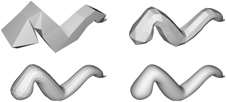
Figure 17.46. A worm subdivided three times with Loop’s subdivision scheme.

A variant of Equation 17.62, which avoids trigonometric functions, is given by Warren and Weimer [1847]:

(17.63)

$\begin{matrix} β (n) = \frac{3}{n (n + 2)} . \end{matrix}$

For regular valences, this gives a $C^{2}$ surface, and $C^{1}$ elsewhere. The resulting surface is hard to distinguish from a regular Loop surface. For a mesh that is not closed, we cannot use the presented subdivision rules. Instead, special rules have to be used for such boundaries. For Loop’s scheme, the reflection rules of Equation 17.60 can be used. This is also treated in Section 17.5.3.

The surface after infinitely many subdivision steps is called the limit surface. Limit surface points and limit tangents can be computed using closed form expressions. The limit position of a vertex is computed [767,1977] using the formula on the first row in Equation 17.61, by replacing $β (n)$ with

(17.64)

$\begin{matrix} γ (n) = \frac{1}{n + \frac{3}{8 β (n)}} . \end{matrix}$

Two limit tangents for a vertex $p^{k}$ can be computed by weighting the immediate neighboring vertices, called the 1-ring or 1-neighborhood, as shown below [767,1067]:

(17.65)

$\begin{matrix} t_{u} = \sum_{i = 0}^{n - 1} cos (2 π i / n) p_{i}^{k}, t_{v} = \sum_{i = 0}^{n - 1} sin (2 π i / n) p_{i}^{k} . \end{matrix}$

The normal is then $n = t_{u} \times t_{v}$ . Note that this often is less expensive [1977] than the methods described in Section 16.3, which need to compute the normals of the neighboring triangles. More importantly, this gives the exact normal at the point.

A major advantage of approximating subdivision schemes is that the resulting surface tends to get fair. Fairness is, loosely speaking, related to how smoothly a curve or surface bends [1239]. A higher degree of fairness implies a smoother curve or surface. Another advantage is that approximating schemes converge faster than interpolating schemes. However, this means that the shapes often shrink. This is most notable for small, convex meshes, such as the tetrahedron shown in Figure 17.47.

Figure 17.47. A tetrahedron is subdivided five times with Loop’s, the $\sqrt{3}$ , and the modified butterfly (MB) scheme [1975]. Loop’s and the $\sqrt{3}$ -scheme [915] are both approximating, while MB is interpolating, where the latter means that the initial vertices are located on the final surface. We cover only approximating schemes in this book due to their popularity in games and offline rendering.

One way to decrease this effect is to use more vertices in the control mesh, i.e., care must be taken while modeling it. Maillot and Stam present a framework for combining subdivision schemes so that the shrinking can be controlled [1106]. A characteristic that can be used to great advantage at times is that a Loop surface is contained inside the convex hull of the original control points [1976].

The Loop subdivision scheme generates a generalized three-directional quartic box spline. ¹ So, for a mesh consisting only of regular vertices, we could actually describe the surface as a type of spline surface. However, this description is not possible for irregular settings. Being able to generate smooth surfaces from any mesh of vertices is one of the great strengths of subdivision schemes. See also Sections 17.5.3 and 17.5.4 for different extensions to subdivision surfaces that use Loop’s scheme.

17.5.2. Catmull-Clark Subdivision

The two most famous subdivision schemes that can handle polygonal meshes (rather than just triangles) are Catmull-Clark [239] and Doo-Sabin [370]. ² Here, we will only briefly present the former. Catmull-Clark surfaces have been used in Pixar’s short film Geri’s Game [347], Toy Story 2, and in all subsequent feature films from Pixar. This subdivision scheme is also commonly used for making models for games, and is probably the most popular one. As pointed out by DeRose et al. [347], Catmull-Clark surfaces tend to generate more symmetrical surfaces. For example, an oblong box results in a symmetrical ellipsoid-like surface, which agrees with intuition. In contrast, a triangular-based subdivision scheme would treat each cube face as two triangles, and would hence generate different results depending on how the square is split.

The basic idea for Catmull-Clark surfaces is shown in Figure 17.48, and an actual example of Catmull-Clark subdivision is shown in Figure 17.41 on page 757.

Figure 17.48. The basic idea of Catmull-Clark subdivision. Each polygon generates a new point, and each edge generates a new point. These are then connected as shown to the right. Weighting of the original points is not shown here.

As can be seen, this scheme only generates faces with four vertices. In fact, after the first subdivision step, only vertices of valence 4 are generated, thus such vertices are called ordinary or regular (compared to valence 6 for triangular schemes).

Following the notation from Halstead et al. [655], let us focus on a vertex $v^{k}$ with n surrounding edge points $e_{i}^{k}$ , where $i = 0 \dots n - 1$ . See Figure 17.49. Now, for each face, a new face point $f^{k + 1}$ is computed as the face centroid, i.e., the mean of the points of the face. Given this, the subdivision rules are [239,655,1977]

(17.66)

$\begin{matrix} \begin{matrix} v^{k + 1} & = \frac{n - 2}{n} v^{k} + \frac{1}{n^{2}} \sum_{j = 0}^{n - 1} e_{j}^{k} + \frac{1}{n^{2}} \sum_{j = 0}^{n - 1} f_{j}^{k + 1}, \\ [3 p t] e_{j}^{k + 1} & = \frac{v^{k} + e_{j}^{k} + f_{j - 1}^{k + 1} + f_{j}^{k + 1}}{4} . \end{matrix} \end{matrix}$

As can be seen, the vertex $v^{k + 1}$ is computed as weighting of the considered vertex, the average of the edge points, and the average of the newly created face points. On the other hand, new edge points are computed by the average of the considered vertex, the edge point, and the two newly created face points that have the edge as a neighbor.

Figure 17.49. Before subdivision, we have the blue vertices and corresponding edges and faces. After one step of Catmull-Clark subdivision, we obtain the red vertices, and all new faces are quadrilaterals. (Illustration after Halstead et al. [655].)

The Catmull-Clark surface describes a generalized bicubic B-spline surface. So, for a mesh consisting only of regular vertices we could actually describe the surface as a bicubic B-spline surface (Section 17.2.7) [1977]. However, this is not possible for irregular mesh settings, and being able to handle these using subdivision surfaces is one of the scheme’s strengths.

Limit positions and tangents are also possible to compute, even at arbitrary parameter values using explicit formulae [1687]. Halstead et al. [655] describe a different approach to computing limit points and normals.

See Section 17.6.3 for a set of efficient techniques that can render Catmull-Clark subdivision surfaces using the GPU.

17.5.3. Piecewise Smooth Subdivision

In a sense, curved surfaces may be considered boring because they lack detail. Two ways to improve such surfaces are to use bump or displacement maps (Section 17.5.4). A third approach, piecewise smooth subdivision, is described here. The basic idea is to change the subdivision rules so that darts, corners, and creases can be used. This increases the range of different surfaces that can be modeled and represented. Hoppe et al. [767] first described this for Loop’s subdivision surfaces. See Figure 17.50 for a comparison of a standard Loop subdivision surface, and one with piecewise smooth subdivision.

Figure 17.50. The top row shows a control mesh, and the limit surface using the standard Loop subdivision scheme. The bottom row shows piecewise smooth subdivision with Loop’s scheme. The lower left image shows the control mesh with tagged edges (sharp) shown in a light gray. The resulting surface is shown to the lower right, with corners, darts, and creases marked. (Image courtesy of Hugues Hoppe.)

To actually be able to use such features on the surface the edges that we want to be sharp are first tagged, so we know where to subdivide differently. The number of sharp edges coming in at a vertex is denoted s. Then the vertices are classified into: smooth ( $s = 0$ ), dart ( $s = 1$ ), crease ( $s = 2$ ), and corner ( $s > 2$ ). Therefore, a crease is a curve on the surface, where the continuity across the curve is $C^{0}$ . A dart is a non-boundary vertex where a crease ends and smoothly blends into the surface. Finally, a corner is a vertex where three or more creases come together. Boundaries can be defined by marking each boundary edge as sharp.

After classifying the various vertex types, Hoppe et al. use a table to determine which mask to use for the various combinations. They also show how to compute limit surface points and limit tangents. Biermann et al. [142] present several improved subdivision rules. For example, when extraordinary vertices are located on a boundary, the previous rules could result in gaps. This is avoided with the new rules. Also, their rules make it possible to specify a normal at a vertex, and the resulting surface will adapt to get that normal at that point. DeRose et al. [347] present a technique for creating soft creases. They allow an edge to first be subdivided as sharp a number of times (including fractions), and after that, standard subdivision is used.

17.5.4. Displaced Subdivision

Bump mapping (Section ) is one way to add detail to otherwise smooth surfaces. However, this is just an illusionary trick that changes the normal or local occlusion at each pixel. The silhouette of an object looks the same with or without bump mapping. The natural extension of bump mapping is displacement mapping [287], where the surface is displaced. This is usually done along the direction of the normal. So, if the point of the surface is $p$ , and its normalized normal is $n$ , then the point on the displaced surface is

(17.67)

$\begin{matrix} s (u, v) = p (u, v) + d (u, v) n (u, v) . \end{matrix}$

The scalar d is the displacement at the point $p$ . The displacement could also be vector-valued [938].

In this section, the displaced subdivision surface [1006] will be presented. The general idea is to describe a displaced surface as a coarse control mesh that is subdivided into a smooth surface that is then displaced along its normals using a scalar field. In the context of displaced subdivision surfaces, $p$ in Equation 17.67 is the limit point on the subdivision surface (of the coarse control mesh), and $n$ is the normalized normal at $p$ , computed as

(17.68)

$\begin{matrix} n = \frac{n^{'}}{| | n^{'} | |}, w h e r e n^{'} = p_{u} \times p_{v}, \end{matrix}$

In Equation 17.68, $p_{u}$ and $p_{v}$ are the first-order derivative of the subdivision surface. Thus, they describe two tangents at $p$ . Lee et al. [1006] use a Loop subdivision surface for the coarse control mesh, and its tangents can be computed using Equation 17.65. Note that the notation is slightly different here; we use $p_{u}$ and $p_{v}$ instead of $t_{u}$ and $t_{v}$ . Equation 17.67 describes the displaced position of the resulting surface, but we also need a normal, $n_{s}$ , on the displaced subdivision surface in order to render it correctly. It is computed analytically as shown below [1006]:

(17.69)

$\begin{matrix} \begin{matrix} n_{s} & = s_{u} \times s_{v}, w h e r e \\ s_{u} & = \frac{\partial s}{\partial u} = p_{u} + d_{u} n + d n_{u} a n d s_{v} = \frac{\partial s}{\partial v} = p_{v} + d_{v} n + d n_{v} . \end{matrix} \end{matrix}$

To simplify computations, Blinn [160] suggests that the third term can be ignored if the displacements are small. Otherwise, the following expressions can be used to compute $n_{u}$ (and similarly $n_{v}$ ) [1006]:

(17.70)

$\begin{matrix} \begin{matrix} {\bar{n}}_{u} & = p_{uu} \times p_{v} + p_{u} \times p_{uv}, \\ n_{u} & = \frac{{\bar{n}}_{u} - ({\bar{n}}_{u} \cdot n) n}{| | n^{'} | |} . \end{matrix} \end{matrix}$

Note that ${\bar{n}}_{u}$ is not any new notation, it is merely a “temporary” variable in the computations. For an ordinary vertex (valence $n = 6$ ), the first and second order derivatives are particularly simple. Their masks are shown in Figure 17.51.

Figure 17.51. The masks for an ordinary vertex in Loop’s subdivision scheme. Note that after using these masks, the resulting sum should be divided as shown. (Illustration after Lee et al. [1006].)

For an extraordinary vertex (valence $n \neq 6$ ), the third term in rows one and two in Equation 17.69 is omitted.

An example using displacement mapping with Loop subdivision is shown in Figure 17.52.

When a displaced surface is far away from the viewer, standard bump mapping could be used to give the illusion of this displacement. Doing so saves on geometry processing. Some bump mapping schemes need a tangent-space coordinate system at the vertex, and the following can be used for that: $(b, t, n)$ , where $t = p_{u} / | | p_{u} | |$ and $b = n \times t$ .

Nießner and Loop [1281] present a similar method as the one presented above by Lee et al., but they use Catmull-Clark surfaces and use direct evaluation of the derivatives on the displacement function, which is faster. They also use the hardware tessellation pipeline (Section ) for rapid tessellation.

Figure 17.52. To the left is a coarse mesh. In the middle, it is subdivided using Loop’s subdivision scheme. The right image shows the displaced subdivision surface. (Image courtesy of Aaron Lee, Henry Moreton, and Hugues Hoppe.)

17.5.5. Normal, Texture, and Color Interpolation

In this section, we will present different strategies for dealing with normals, texture coordinates and color per vertex.

As shown for Loop’s scheme in Section 17.5.1, limit tangents, and thus, limit normals can be computed explicitly. This involves trigonometric functions that may be expensive to evaluate. Loop and Schaefer [1070] present an approximative technique where Catmull-Clark surfaces always are approximated by bicubic Bézier surfaces (Section 17.2.1). For normals, two tangent patches are derived, that is, one in the u-direction and one the v-direction. The normal is then found as the cross product between those vectors. In general, the derivatives of a Bézier patch are computed using Equation 17.35. However, since the derived Bézier patches approximate the Catmull-Clark surface, the tangent patches will not form a continuous normal field. Consult Loop and Schaefer’s paper [1070] on how to overcome these problems. Alexa and Boubekeur [29] argue that it can be more efficient in terms of quality per computation to also subdivide the normals, which gives nicer continuity in the shading. We refer to their paper for the details on how to subdivide the normals. More types of approximations can also be found in Ni et al.’s SIGGRAPH course [1275].

Assume that each vertex in a mesh has a texture coordinate and a color. To be able to use these for subdivision surfaces, we also have to create colors and texture coordinates for each newly generated vertex, too. The most obvious way to do this is to use the same subdivision scheme as we used for subdividing the polygon mesh. For example, you can treat the colors as four-dimensional vectors (RGBA), and subdivide these to create new colors for the new vertices. This is a reasonable way to do it, since the color will have a continuous derivative (assuming the subdivision scheme is at least $C^{1}$ ), and thus abrupt changes in colors are avoided over the surface The same can certainly be done for texture coordinates [347]. However, care must be taken when there are boundaries in texture space. For example, assume we have two patches sharing an edge but with different texture coordinates along this edge. The geometry should be subdivided with the surface rules as usual, but the texture coordinates should be subdivided using boundary rules in this case.

A sophisticated scheme for texturing subdivision surfaces is given by Piponi and Borshukov [1419].

17.6 Efficient Tessellation

To display a curved surface in a real-time rendering context, we usually need to create a triangle mesh representation of the surface. This process is known as tessellation. The simplest form of tessellation is called uniform tessellation. Assume that we have a parametric Bézier patch, $p (u, v)$ , as described in Equation 17.32. We want to tessellate this patch by computing 11 points per patch side, resulting in $10 \times 10 \times 2 = 200$ triangles. The simplest way to do this is to sample the uv-space uniformly. Thus, we evaluate $p (u, v)$ for all $(u_{k}, v_{l}) = (0.1 k, 0.1 l)$ , where both k and l can be any integer from 0 to 10. This can be done with two nested for-loops. Two triangles can be created for the four surface points $p (u_{k}, v_{l})$ , $p (u_{k + 1}, v_{l})$ , $p (u_{k + 1}, v_{l + 1})$ , and $p (u_{k}, v_{l + 1})$ .

While this certainly is straightforward, there are faster ways to do it. Instead of sending tessellated surfaces, consisting of many triangles, over the bus from the CPU to the GPU, it makes more sense to send the curved surface representation to the GPU and let it handle the data expansion. Recall that the tessellation stage is described in Section 3.6. For a quick refresher, see Figure 17.53.

Figure 17.53. Pipeline with hardware tessellation, where the new stages are shown in the middle three (blue) boxes. We use the naming conventions from DirectX here, with the OpenGL counterparts in parenthesis. The hull shader computes new locations of control points and computes tessellation factors as well, which dictates how many triangles the subsequent step should generate. The tessellator generates points in the uv-space, in this case a unit square, and connects them into triangles. Finally, the domain shader computes the positions at each uv-coordinate using the control points.

The tessellator may use a fractional tessellation technique, which is described in the following section. Then follows a section on adaptive tessellation, and finally, we describe how to render Catmull-Clark surfaces and displacement mapped surfaces with tessellation hardware.

17.6.1. Fractional Tessellation

To obtain smoother level of detail for parametric surfaces, Moreton introduced fractional tessellation factors [1240]. These factors enable a limited form of adaptive tessellation, since different tessellation factors can be used on different sides of the parametric surface. Here, an overview of how these techniques work will be presented.

In Figure 17.54, constant tessellation factors for rows and columns are shown on the left, and independent tessellation factors for all four edges on the right. Note that the tessellation factor of an edge is the number of points generated on that edge, minus one. In the patch on the right, the greater of the top and bottom factors is used in the interior for both of these edges, and similarly the greater of the left and right factors is used in the interior. Thus, the basic tessellation rate is $4 \times 8$ . For the sides with smaller factors, triangles are filled in along the edges. Moreton [1240] describes this process in more detail.

Figure 17.54. Left: normal tessellation—one factor is used for the rows, and another for the columns. Right: independent tessellation factors on all four edges. (Illustration after Moreton [1240].)

Figure 17.55. Top: integer tessellation. Middle: fractional tessellation, with the fraction to the right. Bottom: fractional tessellation with the fraction in the middle. This configuration avoids cracks between adjacent patches.

The concept of fractional tessellation factors is shown for an edge in Figure 17.55. For an integer tessellation factor of n, $n + 1$ points are generated at k / n, where $k = 0, \dots, n$ . For a fractional tessellation factor, r, $⌈ r ⌉$ points are generated at k / r, where $k = 0, \dots, ⌊ r ⌋$ . Here, $⌈ r ⌉$ computes the ceiling of r, which is the closest integer toward $+ \infty$ , and $⌊ r ⌋$ computes the floor, which is the closest integer toward $- \infty$ . Then, the rightmost point is just “snapped” to the rightmost endpoint. As can be seen in the middle illustration in Figure 17.55, this pattern in not symmetric. This leads to problems, since an adjacent patch may generate the points in the other direction, and so give cracks between the surfaces. Moreton solves this by creating a symmetric pattern of points, as shown at the bottom of Figure 17.55. See also Figure 17.56 for an example.

Figure 17.56. A patch with the rectangular domain fractionally tessellated. (Illustration after Moreton [1240].)

Figure 17.57. Fractional tessellation of a triangle, with tessellation factors shown. Note that the tessellation factors may not correspond exactly to those produced by actual tessellation hardware. (Illustration after Tatarchuk [1745].)

So far, we have seen methods for tessellating surfaces with a rectangular domain, e.g., Bézier patches. However, triangles can also be tessellated using fractions [1745], as shown in Figure 17.57. Like the quadrilaterals, it is also possible to specify an independent fractional tessellation rate per triangle edge. As mentioned, this enables adaptive tessellation (Section 17.6.2), as illustrated in Figure 17.58, where displacement mapped terrain is rendered.

Once triangles or quadrilaterals have been created, they can be forwarded to the next step in the pipeline, which is treated in the next subsection.

17.6.2. Adaptive Tessellation

Uniform tessellation gives good results if the sampling rate is high enough. However, in some regions on a surface there may not be as great a need for high tessellation as in other regions. This may be because the surface bends more rapidly in some area and therefore may need higher tessellation there, while other parts of the surface are almost flat or far away, and only a few triangles are needed to approximate them. A solution to the problem of generating unnecessary triangles is adaptive tessellation, which refers to algorithms that adapt the tessellation rate depending on some measure (for example curvature, triangle edge length, or some screen size measure). Figure 17.58 shows an example of adaptive tessellation for terrain.

Figure 17.58. Displaced terrain rendering using adaptive fractional tessellation. As can be seen in the zoomed-in mesh to the right, independent fractional tessellation rates are used for the edges of the red triangles, which gives us adaptive tessellation. (Images courtesy of Game Computing Applications Group, Advanced Micro Devices, Inc.)

Figure 17.59. To the left, a crack is visible between the two regions. This is because the right has a higher tessellation rate than the left. The problem lies in that the right region has evaluated the surface where there is a black circle, and the left region has not. The standard solution is shown to the right.

Care must be taken to avoid cracks that can appear between different tessellated regions. See Figure 17.59. When using fractional tessellation, it is common to base the edge tessellation factors on information that comes from only the edge itself, since the edge data are all that is shared between the two connected patches. This is a good start, but due to floating point inaccuracies, there can still be cracks. Nießner et al. [1279] discuss how to make the computations fully watertight, e.g., by making sure that, for an edge, the exact same point is returned regardless of whether tessellation is done from $p_{0}$ to $p_{1}$ , or vice versa.

In this section, we will present some general techniques that can be used to compute fractional tessellation rates, or to decide when to terminate further tessellation and when to split larger patches into a set of smaller ones.

Terminating Adaptive Tessellation

To provide adaptive tessellation, we need to determine when to stop the tessellation, or equivalently how to compute fractional tessellation factors. Either you can use only the information of an edge to determine if tessellation should be terminated, or use information from an entire triangle, or a combination.

It should also be noted that with adaptive tessellation, one can get swimming or popping artifacts from frame to frame if the tessellation factors for a certain edge change too much from one frame to the next. This may be a factor to take into consideration when computing tessellation factors as well. Given an edge, $(a, b)$ , with an associated curve, i.e., a patch edge curve, we can try to estimate how flat the curve is between $a$ and $b$ . See Figure 17.60.

Figure 17.60. The points $a$ and $b$ have already been generated on this surface. The question is: Should a new point, that is $c$ , be generated on the surface?

The midpoint in parametric space between $a$ and $b$ is found, and its three-dimensional counterpart, $c$ , is computed. Finally, the length, l, between $c$ and its projection, $d$ , onto the line between $a$ and $b$ , is computed. This length, l, is used to determine whether the curve segment on that edge if flat enough. If l is small enough, it is considered flat. Note that this method may falsely consider an S-shaped curve segment to be flat. A solution to this is to randomly perturb the parametric sample point [470]. An alternative to using just l is to use the ratio $l / | | a - b | |$ , giving a relative measure [404]. Note that this technique can be extended to consider a triangle as well, where you simply compute the surface point in the middle of the triangle and use the distance from that point to the triangle’s plane. To be certain that this type of algorithm terminates, it is common to set some upper limit on how many subdivisions can be made. When that limit is reached, the subdivision ends. For fractional tessellation, the vector from $c$ to $d$ can be projected onto the screen, and its (scaled) length used as a tessellation rate.

So far we have discussed how to determine the tessellation rate from only the shape of the surface. Other factors that typically are used for on-the-fly tessellation include whether the local neighborhood of a vertex is [769,1935]:

Inside the view frustum.
Frontfacing.
Occupying a large area in screen space.
Close to the silhouette of the object.

These factors will be discussed in turn here. For view frustum culling, one can place a sphere to enclose the edge. This sphere is then tested against the view frustum. If it is outside, we do not subdivide that edge further.

For face culling, the normals at $a$ , $b$ , and possibly $c$ can be computed from the surface description. These normals, together with $a$ , $b$ , and $c$ , define three planes. If all are backfacing, it is likely that no further subdivision is needed for that edge.

There are many different ways to implement screen-space coverage (see also Section ). All methods project some simple object onto the screen and estimate the length or area in screen space. A large area or length implies that tessellation should proceed. A fast estimation of the screen-space projection of a line segment from $a$ to $b$ is shown in Figure 17.61.

Figure 17.61. Estimation of the screen-space projection, s, of the line segment.

First, the line segment is translated so that its midpoint is on the view ray. Then, the line segment is assumed to be parallel to the near plane, n, and the screen-space projection, s, is computed from this line segment. Using the points of the line segment $a^{'}$ and $b^{'}$ to the right in the illustration, the screen-space projection is then

(17.71)

$\begin{matrix} s = \frac{\sqrt{(a^{'} - b^{'}) \cdot (a^{'} - b^{'})}}{v \cdot (a^{'} - e)} . \end{matrix}$

The numerator is simply the length of the line segment. This is divided by the distance from the eye, $e$ , to the line segment’s midpoint. The computed screen-space projection, s, is then compared to a threshold, t, representing the maximum edge length in screen space. Rewriting the previous equation to avoid computing the square root, if the following condition is true, the tessellation should continue:

(17.72)

$\begin{matrix} s > t ⟺ (a^{'} - b^{'}) \cdot (a^{'} - b^{'}) > t^{2} {(v \cdot (a^{'} - e))}^{2} . \end{matrix}$

Note that $t^{2}$ is a constant and so can be precomputed. For fractional tessellation, s from Equation 17.71 can be used as the tessellation rate, possibly with a scaling factor applied. Another way to measure projected edge length is to place a sphere at the center of the edge, make the radius half the edge length, and then use the projection of the sphere as the edge tessellation factor [1283]. This test is proportional to the area, while the test above is proportional to edge length.

Increasing the tessellation rate for the silhouettes is important, since they play a prime role for the perceived quality of the object. Finding if a triangle is near a silhouette edge can be done by testing whether the dot product between the normal at $a$ and the vector from the eye to $a$ is close to zero. If this is true for any of $a$ , $b$ , or $c$ , further tessellation should be done.

For displaced subdivision, Nießner and Loop [1281] use one of the following factors for each base mesh vertex $v$ , which is connected to n edge vectors $e_{i}$ , $i \in {0, 1, \dots, n - 1}$ :

(17.73)

$\begin{matrix} \begin{matrix} f_{1} & = k_{1} \cdot | | c - v | |, \\ f_{2} & = k_{2} \sqrt{\sum e_{i} \times e_{i + 1}}, \\ f_{3} & = k_{3} max (| | e_{0} | |, | | e_{1} | |, \dots, | | e_{n - 1} | |), \end{matrix} \end{matrix}$

where the loop index, i, goes over all n edges $e_{i}$ connected to $v$ , $c$ is the position of the camera, and $k_{i}$ are user-supplied constants. Here, $f_{1}$ is simply based on the distance to the vertex from the camera, $f_{2}$ computes the area of the quads connected to $v$ , and $f_{3}$ uses the largest edge length. The tessellation factor for a vertex is then computed as the maximum of the edge’s two base vertices’ tessellation factors. The inner tessellation factors are computed as the maximum of the opposite edge’s tessellation factor (in u and v). This method can be used with any of the edge tessellation factor methods presented in this section.

Notably, Nießner et al. [1279] recommend using a single global tessellation factor for characters, which depends on the distance to the character. The number of subdivisions is then $⌈ {log}_{2} f ⌉$ , where f is the per-character tessellation factor, which can be computed using any of the methods above.

It is hard to say what methods will work in all applications. The best advice is to test several of the presented heuristics, and combinations of them.

Split and Dice Methods

Cook et al. [289] introduced a method called split and dice, with the goal being to tessellate surfaces so that each triangle becomes pixel-sized, to avoid geometrical aliasing. For real-time purposes, this tessellation threshold should be increased to what the GPU can handle. Each patch is first split recursively into a set of subpatches until it is estimated that if uniform tessellation is used for a certain subpatch, the triangles will have the desired size. Hence, this is also a type of adaptive tessellation.

Imagine a single large patch being used for a landscape. In general, there is no way that fractional tessellation can adapt so that the tessellation rate is higher closer to the camera and lower farther away, for example. The core of split and dice may therefore be useful for real-time rendering, even if the target tessellation rate is to have larger triangles than pixel-sized in our case.

Next, we describe the general method for split and dice in a real-time graphics scenario. Assume that a rectangular patch is used. Then start a recursive routine with the entire parametric domain, i.e., the square from (0, 0) to (1, 1). Using the adaptive termination criteria just described, test whether the surface is tessellated enough. If it is, then terminate tessellation. Otherwise, split this domain into four different equally large squares and call the routine recursively for each of the four subsquares. Continue recursively until the surface is tessellated enough or a predefined recursion level is reached. The nature of this algorithm implies that a quadtree is recursively created during tessellation. However, this will give cracks if adjacent subsquares are tessellated to different levels. The standard solution is to ensure that two adjacent subsquares only differ in one level at most. This is called a restricted quadtree. Then the technique shown to the right in Figure 17.59 is used to fill in the cracks. A disadvantage with this method is that the bookkeeping is more involved.

Liktor et al. [1044] present a variant of split and dice for the GPU. The problem is to avoiding swimming artifacts and popping effects when suddenly deciding to split one more time due to, e.g., the camera having moved closer to a surface. To solve that, they use a fractional split method, inspired by fractional tessellation. This is illustrated in Figure 17.62.

Figure 17.62. Fractional splitting is applied to a cubic Bézier curve. The tessellation rate t is shown for each curve. The split point is the large black circle, which is moved in from the right side of the curve toward the center of the curve. To fractionally split the cubic curve, the black point is smoothly moved toward the curve’s center and the original curve is replaced with two cubic Bézier segments that together generate the original curve. To the right, the same concept is illustrated for a patch, which has been split into four smaller subpatches, where 1.0 indicates that the split point is on the center point of the edge, and 0.0 means that it is at the patch corner. (Illustration after Liktor et al. [1044].)

Since the split is smoothly introduced from one side toward the center of the curve, or toward the center of the patch side, swimming and popping artifacts are avoided. When the termination criteria for the adaptive tessellation have been reached, each remaining subpatch is tessellated by the GPU using fractional tessellation as well.

17.6.3. Fast Catmull-Clark Tessellation

Catmull-Clark surfaces (Section 17.5.2) are frequently used in modeling software and in feature film rendering, and hence it is attractive to be able to render these efficiently using graphics hardware as well. Fast tessellation methods for Catmull-Clark surfaces have been an active research field over recent years. Here, we will present a handful of these methods.

Approximating Approaches

Loop and Schaefer [1070] present a technique to convert Catmull-Clark surfaces into a representation that can be evaluated quickly in the domain shader, without the need to know the polygons’ neighbors.

As mentioned in Section 17.5.2, the Catmull-Clark surface can be described as many small B-spline surfaces when all vertices are ordinary. Loop and Schaefer convert a quadrilateral (quad) polygon in the original Catmull-Clark subdivision mesh to a bi-cubic Bézier surface (Section 17.2.1). This is not possible for non-quadrilaterals, and so we assume that there are no such polygons (recall that after the first step of subdivision there are only quadrilateral polygons). When a vertex has a valence different from four, it is not possible to create a bicubic Bézier patch that is identical to the Catmull-Clark surface. Hence, an approximative representation is proposed, which is exact for quads with valence-four vertices, and close to the Catmull-Clark surface elsewhere. To this end, both geometry patches and tangent patches are used, which will be described next.

The geometry patch is simply a bicubic Bézier patch

with $4 \times 4$ control points. We will describe how these control points are computed. Once this is done, the patch can be tessellated and the domain shader can evaluate the Bézier patch quickly at any parametric coordinate (u, v). So, assuming we have a mesh consisting of only quads with vertices of valence four, we want to compute the control points of the corresponding Bézier patch for a certain quad in the mesh. To that end, the neighborhood around the quad is needed. The standard way of doing this is illustrated in Figure 17.63, where three different masks are shown. These can be rotated and reflected in order to create all the 16 control points. Note that in an implementation the weights for the masks should sum to one, a process that is omitted here for clarity.

Figure 17.63. Left: part of a quad mesh, where we want to compute a Bézier patch for the gray quad. Note that the gray quad has vertices with only valence four. The blue vertices are neighboring quads’ vertices, and the green circles are the control points of the Bézier patch. The following three illustrations show the different masks used to compute the green control points. For example, to compute one of the inner control points, the middle right mask is used, and the vertices of the quad are weighted with the weight shown in the mask.

Figure 17.64. Left: a Bézier patch for the gray quad of the mesh is to be generated. The lower left vertex in the gray quad is extraordinary, since its valence is $n \neq 4$ . The blue vertices are neighboring quads’ vertices, and the green circles are the control points of the Bézier patch. The following three illustrations show the different masks used to compute the green control points.

Figure 17.65. Left: quad structure of a mesh. White quads are ordinary, green have one extraordinary vertex, and blue have more than one. Middle left: geometry patch approximation. Middle right: geometry patches with tangent patches. Note that the obvious (red circle) shading artifacts disappeared. Right: true Catmull-Clark surface. (Image courtesy of Charles Loop and Scott Schaefer, reprinted with permission from Microsoft Corporation.)

The above technique computes a Bézier patch for the ordinary case. When there is at least one extraordinary vertex, we compute an extraordinary patch [1070]. The masks for this are shown in Figure 17.64, where the lower left vertex in the gray quad is an extraordinary vertex.

Note that this results in a patch that approximates the Catmull-Clark subdivision surface, and, it is only $C^{0}$ along edges with an extraordinary vertex. This often looks distracting when shading is added, and hence a similar trick as used for N-patches (Section 17.2.5) is suggested. However, to reduce the computational complexity, two tangent patches are derived: one in the u-direction, and one the v-direction. The normal is then found as the cross product between those vectors. In general, the derivatives of a Bézier patch are computed using Equation 17.35. However, since the derived Bézier patches approximate the Catmull-Clark surface, the tangent patches will not form a continuous normal field. Consult Loop and Schaefer’s paper [1070] on how to overcome these problems. Figure 17.65 shows an example of the types of artifacts that can occur.

Kovacs et al. [931] describe how the method above can be extended to also handle creases and corners (Section 17.5.3), and implement these extensions in Valve’s Source engine.

Feature Adaptive Subdivision and OpenSubdiv

Pixar presented an open-source system called OpenSubdiv that implements a set of techniques called feature adaptive subdivision (FAS) [1279,1280,1282]. The basic approach is rather different from the previous technique just discussed. The foundation of this work lies in that subdivision is equivalent to bicubic B-spline patches (Section 17.2.7) for regular faces, i.e., quads where each vertex is regular, which means that the vertex has valence four. So, subdivision continues recursively only for non-regular faces, up until some maximum subdivision level is reached.

Figure 17.66. Left: recursive subdivision around an extraordinary vertex, i.e., the middle vertex has three edges. As recursion continues, it leaves a band of regular patches (with four vertices, each with four incoming edges) behind. Right: subdivision around a smooth crease indicated by the bold line in the middle. (Illustration after Nießner et al. [1279].)

This is illustrated on the left in Figure 17.66. FAS can also handle creases and semi-smooth creases [347], and the FAS algorithm also needs to subdivide around such creases, which is illustrated on the right in Figure 17.66. The bicubic B-spline patches can be rendered directly using the tessellation pipeline.

The method starts by creating a table using the CPU. This table encodes indices to vertices that need to be accessed during subdivision up to a specified level. As such, the base mesh can be animated since the indices are independent of the vertex positions. As soon as a bicubic B-spline patch is generated, recursion needs not to be continued, which means that the table usually becomes relatively small. The base mesh and the table with indices and additional valence and crease data are uploaded to the GPU once.

To subdivide the mesh one step, new face points are computed first, followed by new edge points, and finally the vertices are updated, and one compute shader is used for each of these types. For rendering, a distinction between full patches and transition patches is made. A full patch (FP) only shares edges with patches of the same subdivision level, and a regular FP is directly rendered as a bicubic B-spline patch using the GPU tessellation pipeline. Subdivision continues otherwise. The adaptive subdivision process ensures that there is at most a difference of one subdivision level between neighboring patches. A transition patch (TP) has a difference in subdivision level against at least one neighbor. To get crack-free renderings, each TP is split into several subpatches as shown in Figure 17.67. In this way, tessellated vertices match along both sides of each edge.

Each type of subpatch is rendered using different hull and domain shaders that implement interpolation variants. For example, the leftmost case in Figure 17.67 is rendered as three triangular B-spline patches. Around extraordinary vertices, another domain shader is used where limit positions and limit normals are computed using the method of Halstead et al. [655]. An example of Catmull-Clark surface rendering using OpenSubdiv is shown in Figure 17.68.

Figure 17.67. Red squares are transition patches, and each has four immediate neighbors, which are either blue (current subdivision level) or green (next subdivision level). This illustration shows the five configurations that can occur, and how they are stitched together. (Illustration after Nießner et al. [1279].)

Figure 17.68. Left: the control mesh in green and red lines with the gray surface (8k vertices) generated using one subdivision step. Middle: the mesh subdivided an additional two steps (102k vertices). Right: the surface generated using adaptive tessellation (28k vertices). (Images generated using OpenSubdiv’s dxViewer.)

The FAS algorithm handles creases, semi-smooth creases, hierarchical details, and adaptive level of detail. We refer to the FAS paper [1279] and Nießner’s PhD thesis [1282] for more details. Schäfer et al. [1547] presents a variant of FAS, called DFAS, which is even faster.

Adaptive Quadtrees

Brainerd et al. [190] present a method called adaptive quadtrees. It is similar to the approximating scheme by Loop and Schaefer [1070] in that a single tessellated primitive is submitted per quad of the original base mesh. In addition, it precomputes a subdivision plan, which is a quadtree that encodes the hierarchical subdivision (similar to feature adaptive subdivision) from an input face, down to some maximum subdivision level. The subdivision plan also contains a list of stencil masks of the control points needed by the subdivided faces.

During rendering, the quadtree is traversed, making it possible to map (u, v)-coordinates to a patch in the subdivision hierarchy, which can be directly evaluated. A quadtree leaf is a subregion of the domain of the original face, and the surface in this subregion can be directly evaluated using the control points in the stencil. An iterative loop is used to traverse the quadtree in the domain shader, whose input is a parametric (u, v)-coordinate. Traversal needs to continue until a leaf node is reached in which the (u, v)-coordinates are located. Depending on the type of node reached in the quadtree, different actions are taken. For example, when reaching a subregion that can be evaluated directly, the 16 control points for its corresponding bicubic B-spline patch are retrieved, and the shader continues with evaluating that patch.

See Figure 17.1 on page 718 for an example rendered using this technique. This method is the fastest to date that renders Catmull-Clark subdivision surfaces exactly, and handles creases and other topological features. An additional advantage of using adaptive quadtrees over FAS is illustrated in Figure 17.69 and further shown in Figure 17.70.

Figure 17.69. Left: hierarchical subdivision according to feature adaptive subdivision (FAS), where each triangle and quad is rendered as a separate tessellated primitive. Right: hierarchical subdivision using adaptive quadtrees, where the entire quad is rendered as a single tessellated primitive. (Illustration after Brainerd et al. [190].)

Adaptive quadtrees also provide more uniform tessellations since there is a one-to-one mapping between each submitted quad and tessellated primitive.

Figure 17.70. Subdivision patches using adaptive quadtrees. Each patch, corresponding to a base mesh face, is surrounded by black curves on the surface and the subdivision steps are illustrated hierarchically inside each patch. As can be seen, there is one patch with uniform color in the center. This implies that it was rendered as a bicubic B-spline patch, while others (with extraordinary vertices) clearly show their underlying adaptive quadtrees. (Image courtesy of Wade Brainerd.)

Table of Contents for
17.3 Implicit Surfaces

17.2.4. PN Triangles

17.2.5. Phong Tessellation

17.2.6. B-Spline Surfaces

17.3 Implicit Surfaces

17.4 Subdivision Curves

17.5 Subdivision Surfaces

17.5.1. Loop Subdivision

17.5.2. Catmull-Clark Subdivision

17.5.3. Piecewise Smooth Subdivision

17.5.4. Displaced Subdivision

17.5.5. Normal, Texture, and Color Interpolation

17.6 Efficient Tessellation

17.6.1. Fractional Tessellation

17.6.2. Adaptive Tessellation

Split and Dice Methods

17.6.3. Fast Catmull-Clark Tessellation

Approximating Approaches

Feature Adaptive Subdivision and OpenSubdiv

Adaptive Quadtrees

Further Reading and Resources

Table of Contents for 17.3 Implicit Surfaces

Create new playlist

Sign In

Sign Up

17.2.4. PN Triangles

17.2.5. Phong Tessellation

17.2.6. B-Spline Surfaces

17.3 Implicit Surfaces

17.4 Subdivision Curves

17.5 Subdivision Surfaces

17.5.1. Loop Subdivision

17.5.2. Catmull-Clark Subdivision

17.5.3. Piecewise Smooth Subdivision

17.5.4. Displaced Subdivision

17.5.5. Normal, Texture, and Color Interpolation

17.6 Efficient Tessellation

17.6.1. Fractional Tessellation

17.6.2. Adaptive Tessellation

Split and Dice Methods

17.6.3. Fast Catmull-Clark Tessellation

Approximating Approaches

Feature Adaptive Subdivision and OpenSubdiv

Adaptive Quadtrees

Further Reading and Resources

Table of Contents for
17.3 Implicit Surfaces