14 Volumetric and Translucency Rendering

Search in book...
Toggle Font Controls
Create new playlist

Name your new playlist

Playlist description (optional)
Sign In

Email address

Password

Forgot Password?

or

Continue with Facebook

Continue with Google
Sign Up

Full Name

Email address

Confirm Email Address

Password

or

Continue with Facebook

Continue with Google

“Those you wish should look farthest away you must make proportionately

bluer; thus, if one is to be five times as distant, make it five times bluer.”

—Leonardo Da Vinci

Participating media is the term used to describe volumes filled with particles. As we can tell by the name, they are media that participate in light transport, in other words they affect light that passes through them via scattering or absorption. When rendering virtual worlds, we usually focus on the solid surfaces, simple yet complex. These surfaces appear opaque because they are defined by light bouncing off of dense participating media, e.g., a dielectric or metal typically modeled using a BRDF. Less dense well-known media are water, fog, steam, or even air, composed of sparse molecules. Depending on its composition, a medium will interact differently with light traveling through it and bouncing off its particles, an event typically referred to as light scattering. The density of particles can be homogeneous (uniform), as in the case of air or water. Or it could be heterogeneous (nonuniform, varying with location in space), as in the case of clouds or steam. Some dense materials often rendered as solid surfaces exhibit high levels of light scattering, such as skin or candle wax. As shown in Section 9.1, diffuse surface shading models are the result of light scattering on a microscopic level. Everything is scattering.

14.1 Light Scattering Theory

In this section, we will describe the simulation and rendering of light in participating media. This is a quantitative treatment of the physical phenomena, scattering and absorption, which were discussed in Sections 9.1.1 and 9.1.2. The radiative transfer equation is described by numerous authors [479,743,818,1413] in the context of path tracing with multiple scattering. Here we will focus on single scattering and build a good intuition about how it works. Single scattering considers only one bounce of light on the particles that constitute the participating media. Multiple scattering tracks many bounces per light path and so is much more complex [243,479]. Results with and without multiple scattering can be seen in Figure 14.51 on page 646. Symbols and units used to represent the participating media properties in scattering equations are presented in Table 14.1. Note that many of the quantities in this chapter, such as σa $σ_{a}$ , σs $σ_{s}$ , σt $σ_{t}$ , p, ρ $ρ$ , v $v$ , and Tr $T_{r}$ are wavelength-dependent, which in practice means that they are RGB quantities.

Table 14.1. Notation used for scattering and participating media. Each of these parameters can depend on the wavelength (i.e., RGB) to achieve colored light absorption or scattering. The units of the phase function are inverse steradians (Section 8.1.1).

14.1.1. Participating Media Material

There are four types of events that can affect the amount of radiance propagating along a ray through a medium. These are illustrated in Figure 14.1 and summarized as:

Absorption (function of σa $σ_{a}$ )—Photons are absorbed by the medium’s matter and transformed into heat or other forms of energy.
Out-scattering (function of σs $σ_{s}$ )—Photons are scattered away by bouncing off particles in the medium matter. This will happen according to the phase function p describing the distribution of light bounce directions.
Emission—Light can be emitted when media reaches a high heat, e.g., a fire’s black-body radiation. For more details about emission, please refer to the course notes by Fong et al. [479].
In-scattering (function of σs $σ_{s}$ )—Photons from any direction can scatter into the current light path after bouncing off particles and contribute to the final radiance. The amount of light in-scattered from a given direction also depends on the phase function p for that light direction.

Figure 14.1. Different events change the radiance along a direction d $d$ in participating media.

To sum up, adding photons to a path is a function of in-scattering σs $σ_{s}$ and emission. Removing photons is a function of extinction σt=σa+σs $σ_{t} = σ_{a} + σ_{s}$ , representing both absorption and out-scattering. As explained by the radiative transfer equation, the set of coefficients represents the derivative of radiance at position x $x$ and toward direction v $v$ relative to L(x,v) $L (x, v)$ . That is why these coefficients’ values are all in the range [0,+∞] $[0, + \infty]$ . See the notes by Fong et al. [479] for details. The scattering and absorption coefficients determine the medium’s albedo ρ $ρ$ , defined as

(14.1)

ρ = σ s σ s + σ a = σ s σ t,

$\begin{matrix} ρ = \frac{σ_{s}}{σ_{s} + σ_{a}} = \frac{σ_{s}}{σ_{t}}, \end{matrix}$

which represents the importance of scattering relative to absorption in a medium for each visible spectrum range considered, i.e., the overall reflectiveness of the medium. The value of ρ $ρ$ is within the range [0, 1]. A value close to 0 indicates that most of the light is absorbed, resulting in a murky medium, such as dark exhaust smoke. A value close to 1 indicates that most of the light is scattered instead of being absorbed, resulting in a brighter medium, such as air, clouds, or the earth’s atmosphere.

As discussed in Section 9.1.2, the appearance of a medium is a combination of its scattering and absorption properties. Coefficient values for real-world participating media have been measured and published [1258]. For instance, milk has high scattering values, producing a cloudy and opaque appearance. Milk also appears white thanks to a high albedo ρ>0.999 $ρ > 0.999$ . On the other hand, red wine features almost no scattering but instead high absorption, giving it a translucent and colored appearance. See the rendered liquids in Figure 14.2, and compare to the photographed liquids in Figure 9.8 on page 301.

Figure 14.2. Rendered wine and milk, respectively, featuring absorption and scattering at different concentrations. (Images courtesy of Narasimhan et al. [1258].)

Each of these properties and events are wavelength-dependent. This dependence means that in a given medium, different light frequencies may be absorbed or scattered with differing probabilities. In theory, to account for this we should use spectral values in rendering. For the sake of efficiency, in real-time rendering (and with a few exceptions [660] in offline rendering as well) we use RGB values instead. Where possible, the RGB values of quantities such as σa $σ_{a}$ and σs $σ_{s}$ should be precomputed from spectral data using color-matching functions (Section 8.1.3).

In earlier chapters, due to the absence of participating media, we could assume that the radiance entering the camera was the same as the radiance leaving the closest surface. More precisely, we assumed (on page 310) that Li(c,−v)=Lo(p,v) $L_{i} (c, - v) = L_{o} (p, v)$ , where c $c$ is the camera position, p $p$ is the intersection point of the closest surface with the view ray, and v $v$ is the unit view vector pointing from p $p$ to c $c$ .

Figure 14.3. Illustration of single scattering integration from a punctual light source. Sample points along the view ray are shown in green, a phase function for one point is shown in red, and the BRDF for an opaque surface S is shown in orange. Here, lc $l_{c}$ is the direction vector to the light center, plight $p_{l i g h t}$ is the position of the light, p is the phase function, and the function v $v$ is the visibility term.

Once participating media are introduced, this assumption no longer holds and we need to account for the change in radiance along the view ray. As an example, we will now describe the computations involved in evaluating scattered light from a punctual light source, i.e., a light source represented by a single infinitesimal point (Section 9.4):

(14.2)

L i (c, - v) = T r (c, p) L o (p,}} v) + \int | | p - c | | t = 0 T r (c, c - v t) L scat (c - v t,}} v) σ s d t,

$\begin{matrix} L_{i} (c, - v) = T_{r} (c, p) L_{o} (p,}} v) + \int_{t = 0}^{| | p - c | |} T_{r} (c, c - v t) L_{scat} (c - v t,}} v) σ_{s} d t, \end{matrix}$

where Tr(c,x) $T_{r} (c, x)$ is the transmittance between a given point x $x$ and the camera position c $c$ (Section 14.1.2) and Lscat(x,}}v) $L_{scat} (x,}} v)$ is the light scattered along the view ray (Section 14.1.3) at a given point x $x$ on the ray. The different components of the calculation are shown in Figure 14.3 and explained in the following subsections. More details about how Equation 14.2 is derived from the radiative transfer equation can be found in the course notes by Fong et al. [479].

14.1.2. Transmittance

The transmittance Tr $T_{r}$ represents the ratio of light that is able to get through a medium over a certain distance according to

(14.3)

T r (x a, x b) = e - τ, where τ = \int x b x = x a σ t (x) | | d x | | .

$\begin{matrix} T_{r} (x_{a}, x_{b}) = e^{- τ}, where τ = \int_{x = x_{a}}^{x_{b}} σ_{t} (x) | | d x | | . \end{matrix}$

This relationship is also known as the Beer-Lambert Law. The optical depth τ $τ$ is unitless and represents the amount of light attenuation.

The higher the extinction or distance traversed, the larger the optical depth will be and, in turn, the less light will travel through the medium. An optical depth τ=1 $τ = 1$ will remove approximately 60% $60 %$ of the light. For instance, if σt=(0.5,1,2) $σ_{t} = (0.5, 1, 2)$ in RGB, then the light coming through depth d=1 $d = 1$ meter will be Tr=e−dσt≈(0.61,0.37,0.14) $T_{r} = e^{- d σ_{t}} \approx (0.61, 0.37, 0.14)$ . This behavior is presented in Figure 14.4. Transmittance needs to be applied on

(i) the radiance Lo(p,v) $L_{o} (p, v)$ from opaque surfaces, (ii) the radiance Lscat(x,v) $L_{scat} (x, v)$ resulting from an in-scattering event, and (iii) each path from a scattering event to the light source. Visually, (i) will result in some fog-like occlusion of surfaces, (ii) will result in occlusion of scattered light, giving another visual cue about the media thickness (see Figure 14.6), and (iii) will result in volumetric self-shadowing by the participating media (see Figure 14.5). Since σt=σa+σs $σ_{t} = σ_{a} + σ_{s}$ , it is expected that the transmittance is influenced by both the absorption and out-scattering components.

Figure 14.4. Transmittance as a function of depth, with σt=(0.5,1.0,2.0) $σ_{t} = (0.5, 1.0, 2.0)$ . As expected, a lower extinction coefficient for the red component leads to more red color being transmitted.

14.1.3. Scattering Events

Integrating in-scattering from punctual light sources in a scene for a given position x $x$ and from direction v $v$ can be done as follows:

(14.4)

L scat (x, v) = π \sum n i = 1 p (v, l c i) v (x, p l i g h t i) c l i g h t i (| | x - p l i g h t i | |),

$\begin{matrix} L_{scat} (x, v) = π \sum_{i = 1}^{n} p (v, l_{c_{i}}) v (x, p_{l i g h t_{i}}) c_{l i g h t_{i}} (| | x - p_{l i g h t_{i}} | |), \end{matrix}$

where n is the number of lights, p() is the phase function, v() $v ()$ is the visibility function, lci $l_{c_{i}}$ is the direction vector to the ith light, and plighti $p_{l i g h t_{i}}$ is the position of the ith light. In addition, clighti() $c_{l i g h t_{i}} ()$ is the radiance from the ith light as a function of the distance to its position, using the definition from Section 9.4 and the inverse square falloff function from Section 5.2.2. The visibility function v(x,plighti) $v (x, p_{l i g h t_{i}})$ represents the ratio of light reaching a position x $x$ from a light source at plighti $p_{l i g h t_{i}}$ according to

(14.5)

v (x, p l i g h t i) = s h a d o w M a p (x, p l i g h t i) \cdot v o l S h a d (x, p l i g h t i),

$\begin{matrix} v (x, p_{l i g h t_{i}}) = s h a d o w M a p (x, p_{l i g h t_{i}}) \cdot v o l S h a d (x, p_{l i g h t_{i}}), \end{matrix}$

where volShad(x,plighti)=Tr(x,plighti) $v o l S h a d (x, p_{l i g h t_{i}}) = T_{r} (x, p_{l i g h t_{i}})$ . In real-time rendering, shadows result from two kinds of occlusion: opaque and volumetric. Shadows from opaque objects ( shadowMap $s h a d o w M a p$ ) are traditionally computed by using shadow mapping or other techniques from Chapter 7.

Figure 14.5. Example of volumetric shadows from a Stanford bunny made of participating media [744]. Left: without volumetric self-shadowing; middle: with self-shadowing; right: with shadows cast on other scene elements. (Model courtesy of the Stanford Computer Graphics Laboratory.)

The volumetric shadow term volShad(x,plighti) $v o l S h a d (x, p_{l i g h t_{i}})$ of Equation 14.5 represents the transmittance from light source position plighti $p_{l i g h t_{i}}$ to sampled point x $x$ , with values in the range [0, 1]. Occlusion produced by a volume is a crucial component of volumetric rendering, where the volume element can self-shadow or cast shadows on other scene elements. See Figure 14.5. This result is usually achieved by performing ray marching along the primary ray from the eye through the volume to the first surface, and then along a secondary ray path from each of these samples toward each light source. “Ray marching” refers to the act of sampling the path between two points using n samples, integrating scattered light and transmittance along the way. See Section 6.8.1 for more details on this method of sampling, which in that case was for rendering a heightfield. Ray marching is similar for three-dimensional volumes, with each ray progressing step by step and sampling the volume material or lighting at each point along the way. See Figure 14.3, which shows sample points on a primary ray in green and secondary shadow rays in blue. Many other publications also describe ray marching in detail [479,1450,1908].

Being of O(n2) $O (n^{2})$ complexity, where n is the number of samples along each path, ray marching quickly becomes expensive. As a trade-off between quality and performance, specific volumetric shadow representation techniques can be used to store transmittance for outgoing directions from a light. These techniques will be explained in the appropriate sections throughout the rest of this chapter.

Figure 14.6. Stanford dragon with increasing media concentration. From left to right: 0.1, 1.0, and 10.0, with σs=(0.5,1.0,2.0) $σ_{s} = (0.5, 1.0, 2.0)$ . (Model courtesy of the Stanford Computer Graphics Laboratory.)

To gain some intuition about the behavior of light scattering and extinction within a medium, consider σs=(0.5,1,2) $σ_{s} = (0.5, 1, 2)$ and σa=(0,0,0) $σ_{a} = (0, 0, 0)$ . For a short light path within the medium, in-scattering events will dominate over extinction, e.g., out-scattering in this case, where Tr≈1 $T_{r} \approx 1$ for a small depth. The material will appear blue, since this channel’s σs $σ_{s}$ value is highest. The deeper that light penetrates into the medium, the fewer photons will get through, due to extinction. In this case, the transmittance color from extinction will start to dominate. This can be explained by the fact that we have σt=σs $σ_{t} = σ_{s}$ , since σa=(0,0,0) $σ_{a} = (0, 0, 0)$ . As a result, Tr=e−dσt $T_{r} = e^{- d σ_{t}}$ will decrease much faster than the linear integration of scattered light as a function of the optical depth dσs $d σ_{s}$ using Equation 14.2. For this example, the red light channel will be less subject to extinction through the medium, since this channel’s σt $σ_{t}$ value is lowest, so it will dominate. This behavior is depicted in Figure 14.6, and is exactly what happens in the atmosphere and sky. When the sun is high (e.g., short light path through the atmosphere, perpendicular to the ground), blue light scatters more, giving the sky its natural blue color. However, when the sun is at the horizon, so that there is a long light path through the atmosphere, the sky will appear redder since more red light is transmitted. This results in the beautiful sunrise and sunset transitions we all know. See Section 14.4.1 for more details about the atmosphere’s material composition. For another example of this effect, see the opalescent glass on the right side of Figure 9.6 on page 299.

14.1.4. Phase Functions

A participating medium is composed of particles with varying radii. The distribution of the size of these particles will influence the probability that light will scatter in a given direction, relative to the light’s forward travel direction. The physics behind this behavior is explained in Section 9.1.

Figure 14.7. Illustration of a phase function (in red) and its influence on scattered light (in green) as a function of θ $θ$ .

Describing the probability and distribution of scattering directions at a macro level is achieved using a phase function when evaluating in-scattering, as shown in Equation 14.4. This is illustrated in Figure 14.7. The phase function in red is expressed using the parameter θ $θ$ as the angle between the light’s forward travel path in blue and toward direction v $v$

in green. Notice the two main lobes in this phase function example: a small backward-scattering lobe in the opposite direction of the light path, and a large forward-scattering lobe. Camera B is in the direction of the large forward-scattering lobe, so it will receive much more scattered radiance as compared to camera A. To be energy-conserving and -preserving, i.e., no energy gain or loss, the integration of a phase function over the unit sphere must be 1.

A phase function will change the in-scattering at a point according to the directional radiance information reaching that point. The simplest function is isotropic: Light will be scattered uniformly in all directions. This perfect but unrealistic behavior is presented as

(14.6)

p (θ) = 1 4 π,

$\begin{matrix} p (θ) = \frac{1}{4 π}, \end{matrix}$

where θ $θ$ is the angle between the incoming light and out-scattering directions, and 4π $4 π$ is the area of the unit sphere.

Physically based phase functions depend on the relative size sp $s_{p}$ of a particle according to

(14.7)

s p = 2 π r λ,

$\begin{matrix} s_{p} = \frac{2 π r}{λ}, \end{matrix}$

where r is the particle radius and λ $λ$ the considered wavelength [743]:

When sp≪1 $s_{p} ≪ 1$ , there is Rayleigh scattering (e.g., air).
When sp≈1 $s_{p} \approx 1$ , there is Mie scattering.
When sp≫1 $s_{p} ≫ 1$ , there is geometric scattering.

Figure 14.8. Polar plot of the Rayleigh phase as a function of θ $θ$ . The light is coming horizontally from the left, and the relative intensity is shown for angle θ $θ$ , measured counterclockwise from the x-axis. The chance of forward and backward scattering is the same.

Rayleigh Scattering

Lord Rayleigh (1842–1919) derived terms for the scattering of light from molecules in the air. These expressions are used, among other applications, to describe light scattering in the earth’s atmosphere. This phase function has two lobes, as shown in Figure 14.8, referred to as backward and forward scattering, relative to the light direction.

This function is evaluated at θ $θ$ , the angle between the incoming light and out-scattering directions. The function is

(14.8)

p (θ) = 3 16 π (1 + cos 2 θ) .

$\begin{matrix} p (θ) = \frac{3}{16 π} (1 + {cos}^{2} θ) . \end{matrix}$

Rayleigh scattering is highly wavelength-dependent. When viewed as a function of the light wavelength λ $λ$ , the scattering coefficient σs $σ_{s}$ for Rayleigh scattering is proportional to the inverse fourth power of the wavelength:

(14.9)

σ s (λ) \propto 1 λ 4 .

$\begin{matrix} σ_{s} (λ) \propto \frac{1}{λ^{4}} . \end{matrix}$

This relationship means that short-wavelength blue or violet light is scattered much more than long-wavelength red light. The spectral distribution from Equation 14.9 can be converted to RGB using spectral color-matching functions (Section 8.1.3): σs=(0.490,1.017,2.339) $σ_{s} = (0.490, 1.017, 2.339)$ . This value is normalized to a luminance of 1, and should be scaled according to the desired scattering intensity. The visual effects resulting from blue light being scattered more in the atmosphere are explained in Section 14.4.1.

Mie Scattering

Mie scattering [776] is a model that can be used when the size of particles is about the same as the light’s wavelength. This type of scattering is not wavelength-dependent. The MiePlot software is useful for simulating this phenomenon [996]. The Mie phase function for a specific particle size is typically a complex distribution with strong and sharp directional lobes, i.e., representing a high probability to scatter photons in specific directions relative to the photon travel direction. Computing such phase functions for volume shading is computationally expensive, but fortunately it is rarely needed. Media typically have a continuous distribution of particle sizes. Averaging the Mie phase functions for all these different sizes results in a smooth average phase function for the overall medium. For this reason, relatively smooth phase functions can be used to represent Mie scattering.

One phase function commonly used for this purpose is the Henyey-Greenstein (HG) phase function, which

was originally proposed to simulate light scattering in interstellar dust [721]. This function cannot capture the complexity of every real-world scattering behavior, but it can be a good match to represent one of the phase function lobes [1967], i.e., toward the main scatter direction. It can be used to represent any smoke, fog, or dust-like participating media. Such media can exhibit strong backward or forward scattering, resulting in large visual halos around light sources. Examples include spotlights in fog and the strong silver-lining effect at the edges of clouds in the sun’s direction.

The HG phase function can represent more complex behavior than Rayleigh scattering and is evaluated using

(14.10)

p h g (θ, g) = 1 - g 2 4 π ( 1 + g 2 - 2 g cos θ ) 1.5 .

$\begin{matrix} p_{hg} (θ, g) = \frac{1 - g^{2}}{4 π {(1 + g^{2} - 2 g cos θ)}^{1.5}} . \end{matrix}$

It can result in varied shapes, as shown in Figure 14.9. The g parameter can be used to represent backward ( g<0 $g < 0$ ), isotropic ( g=0 $g = 0$ ), or forward ( g>0 $g > 0$ ) scattering, with g in [−1,1] $[- 1, 1]$ . Examples of scattering results using the HG phase function are shown in Figure 14.10.

Figure 14.9. Polar plot of the Henyey-Greenstein (in blue) and Schlick approximation (in red) phase as a function of θ $θ$ . The light is coming horizontally from the left. Parameter g increases from 0 to 0.3 and 0.6, resulting in a strong lobe to the right, meaning that light will be scattered more along its forward path, from the left to the right.

A faster way to obtain similar results to the Henyey-Greenstein phase function is to use an approximation proposed by Blasi et al. [157], which is usually named for the third author as the Schlick phase function:

(14.11)

p (θ, k) = 1 - k 2 4 π ( 1 + k cos θ ) 2, where k \approx 1.55 g - 0.55 g 3 .

$\begin{matrix} p (θ, k) = \frac{1 - k^{2}}{4 π {(1 + k cos θ)}^{2}}, where k \approx 1.55 g - 0.55 g^{3} . \end{matrix}$

It does not include any complex power function but instead only a square, which is much faster to evaluate. In order to map this function onto the original HG phase function, the k parameter needs to be computed from g. This has to be done only once for participating media having a constant g value. In practical terms, the Schlick phase function is an excellent energy-conserving approximation, as shown in Figure 14.9.

It is also possible to blend multiple HG or Schlick phase functions in order to represent a more complex range of general phase functions [743]. This allows us to represent a phase function having strong forward- and backward-scattering lobes at the same time, similar to how clouds behave, as described and illustrated in Section 14.4.2.

Figure 14.10. Participating-media Stanford bunny showing HG phase function influence, with g ranging from isotropic to strong forward scattering. From left to right: g = 0.0, 0.5, 0.9, 0.99, and 0.999. The bottom row uses a ten-times denser participating media. (Model courtesy of the Stanford Computer Graphics Laboratory.)

Geometric Scattering

Geometric scattering happens with particles significantly larger than the light’s wavelength. In this case, light can refract and reflect within each particle. This behavior can require a complex scattering phase function to simulate it on a macro level. Light polarization can also affect this type of scattering. For instance, a real-life example is the visual rainbow effect. It is caused by internal reflection of light inside water particles in the air, dispersing the sun’s light into a visible spectrum over a small visual angle ( ∼3 $\sim 3$ degrees) of the resulting backward scattering. Such complex phase functions can be simulated using the MiePlot software [996]. An example of such a phase function is described in Section 14.4.2.

14.2 Specialized Volumetric Rendering

This section presents algorithms for rendering volumetric effects in a basic, limited way. Some might even say these are old school tricks, often relying on ad hoc models. The reason they are used is that they still work well.

14.2.1. Large-Scale Fog

Figure 14.11. Fog used to accentuate a mood. (Image courtesy of NVIDIA Corporation.)

Fog can be approximated as a depth-based effect. Its most basic form is the alpha blending of the fog color on top of a scene according to the distance from the camera, usually called depth fog. This type of effect is a visual cue to the viewer. First, it can increase the level of realism and drama, as seen in Figure 14.11. Second, it is an important depth cue helping the viewer of a scene determine how far away objects are located. See Figure 14.12. Third, it can be used as a form of occlusion culling. If objects are completely occluded by the fog when too far away, their rendering can safely be skipped, increasing application performance.

One way to represent an amount of fog is to have f in [0, 1] representing a transmittance, i.e., f=0.1 $f = 0.1$ means 10% $10 %$ of the background surface is visible. Assuming that the input color of a surface is ci $c_{i}$ and the fog color is cf $c_{f}$ , then the final color, c $c$ , is determined by

(14.12)

c = f c i + (1 - f) c f .

$\begin{matrix} c = f c_{i} + (1 - f) c_{f} . \end{matrix}$

The value f can be evaluated in many different ways. The fog can increase linearly using

(14.13)

f = z end - z s z end - z start,

$\begin{matrix} f = \frac{z_{end} - z_{s}}{z_{end} - z_{start}}, \end{matrix}$

where zstart $z_{start}$ and zend $z_{end}$ are user parameters that determine where the fog is to start and end (i.e., become fully foggy), and zs $z_{s}$ is the linear depth from the viewer to the surface where fog is to be computed. A physically accurate way to evaluate fog transmittance is to have it increase exponentially with distance, thus following the Beer-Lambert Law for transmittance (Section 14.1.2). This effect can be achieved using

(14.14)

f = e - d f z s,

$\begin{matrix} f = e^{- d_{f} z_{s}}, \end{matrix}$

where the scalar df $d_{f}$ is a user parameter that controls the density of the fog. This traditional large-scale fog is a coarse approximation to the general simulation of light scattering and absorption within the atmosphere (Section 14.4.1), but it is still used in games today to great effect. See Figure 14.12.

Figure 14.12. Fog is used in this image of a level from Battlefield 1

This is how hardware fog was exposed in legacy OpenGL and DirectX APIs. It is still worthwhile to consider using these models for simpler use cases on hardware such as mobile devices. Many current games rely on more advanced post-processing for atmospheric effects such as fog and light scattering. One problem with fog in a perspective view is that the depth buffer values are computed in a nonlinear fashion (Section 23.7). It is possible to convert the nonlinear depth buffer values back to linear depths zs $z_{s}$ using inverse projection matrix mathematics [1377]. Fog can then be applied as a full-screen pass using a pixel shader, enabling more advanced results to be achieved, such as height-dependent fog or underwater shading.

Height fog represents a single slab of participating media with a parameterized height and thickness. For each pixel on screen, the density and scattered light is evaluated as a function of the distance the view ray has traveled through the slab before hitting a surface.

Wenzel [1871] proposes a closed-form solution evaluating f for an exponential fall-off of participating media within the slab. Doing so results in a smooth fog transition near the edges of the slab. This is visible in the background fog on the left side of Figure 14.12.

Many variations are possible with depth and height fog. The color cf $c_{f}$ can be a single color, be read from a cube map sampled using the view vector, or even can be the result of complex atmospheric scattering with a per-pixel phase function applied for directional color variations [743]. It is also possible to combine depth fd $f_{d}$ and height fh $f_{h}$ fog transmittance using f=fdfh $f = f_{d} f_{h}$ and have both types of fog interleaved together in a scene.

Depth and height fog are large-scale fog effects. One might want to render more local phenomena such as separated fog areas, for example, in caves or around a few tombs in a cemetery. Shapes such as ellipsoids or boxes can be used to add local fog where needed [1871]. These fog elements are rendered from back to front using their bounding boxes. The front df $d_{f}$ and back db $d_{b}$ intersection along the view vector of each shape is evaluated in the pixel shader. Using volume depth as d=max(0,min(zs,db)−df) $d = max (0, min (z_{s}, d_{b}) - d_{f})$ , where zs $z_{s}$ is the linear depth representing the closest opaque surface, it is possible to evaluate a transmittance Tr $T_{r}$ (Section 14.1.2), with coverage as α=1.0−Tr $α = 1.0 - T_{r}$ . The amount of scattered light cf $c_{f}$ to add on top can then be evaluated as αcf $α c_{f}$ . To allow more varied shapes evaluated from meshes, Oat and Scheuermann [1308] give a clever single-pass method of computing both the closest entry point and farthest exit point in a volume. They save the surface distance, ds $d_{s}$ , to a surface in one channel, and 1−ds $1 - d_{s}$ in another channel. By setting the alpha blending mode to save the minimum value found, after the volume is rendered, the first channel will have the closest value df $d_{f}$ and the second channel will have the farthest value db $d_{b}$ , encoded as 1−d $1 - d$ , allowing recovery of d.

Water is a participating medium and, as such, exhibits the same type of depth-based color attenuation. Coastal water has a transmittance of about (0.3, 0.73, 0.63) per meter [261], thus using Equation 14.23 we can recover σt=(1.2,0.31,0.46) $σ_{t} = (1.2, 0.31, 0.46)$ . When rendering dark water using an opaque surface, it is possible to enable the fog logic when the camera is under the water surface, and to turn it off when above. A more advanced solution has been proposed by Wenzel [1871]. If the camera is under water, scattering and transmittance are integrated until a solid or the water surface is hit. If above water, these are integrated from only the distance between the water’s top surface to the solid geometry of the seabed.

14.2.2. Simple Volumetric Lighting

Light scattering within participating media can be complex to evaluate. Thankfully, there are many efficient techniques that can be used to approximate such scattering convincingly in many situations.

The simplest way to obtain volumetric effects is to render transparent meshes blended over the framebuffer. We refer to this as a splatting approach (Section ). To render light shafts shining through a window, through a dense forest, or from a spotlight, one solution is to use camera-aligned particles with a texture on each. Each textured quad is stretched in the direction of the light shaft while always facing the camera (a cylinder constraint).

Figure 14.13. Volumetric light scattering from light sources evaluated using the analytical integration from the code snippet on page 603. It can be applied as a post effect assuming homogeneous media (left) or on particles, assuming each of them is a volume with depth (right). (Image courtesy of Miles Macklin [1098].)

The drawback with mesh splatting approaches is that accumulating many transparent meshes will increase the required memory bandwidth, likely causing a bottleneck, and the textured quad facing the camera can sometimes be visible. To work around this issue, post-processing techniques using closed-form solutions to light single scattering have been proposed. Assuming a homogeneous and spherical uniform phase function, it is possible to integrate scattered light with correct transmittance along a path assuming a constant medium. The result is visible in Figure 14.13. An example implementation of this technique is shown here in a GLSL shader code snippet [1098]:

float inScattering (vec3 rayStart , vec3 rayDir ,vec3 lightPos , float rayDistance ){// Calculate coefficients .

where rayStart is the ray start position, rayDir is the ray normalized direction, rayDistance the integration distance along the ray, and lightPos the light source position. The solution by Sun et al. [1722] additionally takes into account the scattering coefficient σs $σ_{s}$ . It also describes how the diffuse and specular radiance bouncing off Lambertian and Phong surfaces should be affected by the fact that the light would have scattered in non-straight paths before hitting any surface. In order to take into account transmittance and phase functions, a more ALU-heavy solution can be used [1364]. All these models are effective at what they do, but are not able to take into account shadows from depth maps or heterogeneous participating media.

It is possible to approximate light scattering in screen space by relying on a technique known as bloom [539,1741]. Blurring the framebuffer and adding a small percentage of it back onto itself [44] will make every bright object leak radiance around it. This technique is typically used to approximate imperfections in camera lenses, but in some environments, it is an approximation that works well for short distances and non-occluded scattering. Section 12.3 describes bloom in more detail.

Dobashi et al. [359] present a method of rendering large-scale atmospheric effects using a series of planes sampling the volume. These planes are perpendicular to the view direction and are rendered from back to front. Mitchell [1219] also proposes the same approach to render spotlight shafts, using shadow maps to cast volumetric shadows from opaque objects. Rendering volume by splatting slices is described in detail in Section 14.3.1.

Figure 14.14. Light shafts rendered using a screen-space post-process. (Image courtesy of Kenny Mitchell [1225].)

Mitchell [1225] and Rohleder and Jamrozik [1507] present an alternative method working in screen space; see Figure 14.14. It can be used to render light shafts from a distant light such as the sun. First, a fake bright object is rendered around the sun on the far plane in a buffer cleared to black, and a depth buffer test is used to accept non-occluded pixels. Second, a directional blur is applied on the image in order to leak the previously accumulated radiance outward from the sun. It is possible to use a separable filtering technique (Section 12.1) with two passes, each using n samples, to get the same blur result as n2 $n^{2}$ samples but rendered faster [1681]. To finish, the final blurred buffer can be added onto the scene buffer. The technique is efficient and, despite the drawback that only the light sources visible on screen can cast light shafts, it provides a significant visual result at a small cost.

14.3 General Volumetric Rendering

In this section, we present volumetric rendering techniques that are more physically based, i.e., that try to represent the medium’s material and its interaction with light sources (Section 14.1.1). General volumetric rendering is concerned with spatially varying participating media, often represented using voxels (Section 13.10), with volumetric light interactions resulting in visually complex scattering and shadowing phenomena. A general volumetric rendering solution must also account for the correct composition of volumes with other scene elements, such as opaque or transparent surfaces. The spatially varying media’s properties might be the result of a smoke and fire simulation that needs to be rendered in a game environment, together with volumetric light and shadow interactions. Alternately, we may wish to represent solid materials as semitransparent volumes, for applications such as medical visualization.

14.3.1. Volume Data Visualization

Volume data visualization is a tool used for the display and analysis of volume data, usually scalar fields. Computer tomography (CT) and magnetic resonance image (MRI) techniques can be used to create clinical diagnostic images of internal body structures. A data set may be, say, 2563 $256^{3}$ voxels, each location holding one or more values. This voxel data can be used to form a three-dimensional image. Voxel rendering can show a solid model, or make various materials (e.g., the skin and skull) appear partially or fully transparent. Cutting planes can be used to show only a sub-volume or parts of the source data. In addition to its use for visualization in such diverse fields as medicine and oil prospecting, volumetric rendering can also produce photorealistic imagery.

There are many voxel rendering techniques [842]. It is possible to use regular path tracing or photon mapping to visualize volumetric data under complex lighting environments. Several less-expensive methods have been proposed to achieve real-time performance.

Figure 14.15. A volume is rendered by a series of slices parallel to the view plane. Some slices and their intersection with the volume are shown on the left. The middle shows the result of rendering just these slices. On the right the result is shown when a large series of slices are rendered and blended. (Figures courtesy of Christof Rezk-Salama, University of Siegen, Germany.)

For solid objects, implicit surface techniques can be used to turn voxels into polygonal surfaces, as described in Section 17.3. For semitransparent phenomena, the volume data set can be sampled by a set of equally spaced slices in layers perpendicular to the view direction. Figure 14.15 shows how this works. It is also possible to render opaque surfaces with this approach [797]. In this case, the solid volume is considered present when the density is greater than a given threshold, and the normal n $n$ can be evaluated as the three-dimensional gradient of the density field.

For semitransparent data, it is possible to store color and opacity per voxel. To reduce the memory footprint and enable users to control the visualization, transfer functions have been proposed. A first solution is to map a voxel density scalar to color and opacity using a one-dimensional transfer texture. However, this does not allow identifying specific material transitions, for instance, human sinuses bone-to-air or bone-to-soft tissue, independently, with separate colors. To solve this issue, Kniss et al. [912] suggest using a two-dimensional transfer function that is indexed based on density d and the gradient length of the density field ||▽d|| $||▿ d||$ . Regions of change have high gradient magnitudes. This approach results in more meaningful colorization of density transitions. See Figure 14.16.

Figure 14.16. Volume material and opacity evaluated using a one-dimensional (left) and two-dimensional (right) transfer function [912]. In the second case, it is possible to maintain the brown color of the trunk without having it covered with the green color of lighter density representing the leaves. The bottom part of the image represents the transfer functions, with the x-axis being density and the y-axis the gradient length of the density field ||▽d|| $||▿ d||$ . (Image courtesy of Joe Michael Kniss [912].)

Figure 14.17. Volumetric rendering with forward subsurface scattering using light propagation through half-angle slices. (Image courtesy of Ikits et al. [797].)

Ikits et al. [797] discuss this technique and related matters in depth. Kniss et al. [913] extend this approach, instead slicing according to the half-angle. Slices are still rendered back to front but are oriented halfway between the light and view directions. Using this approach, it is possible to render radiance and occlusion from the light’s point of view and accumulate each slice in view space. The slice texture can be used as input when rendering the next slice, using occlusion from the light direction to evaluate volumetric shadows, and using radiance to estimate multiple scattering, i.e., light bouncing multiple times within a medium before reaching the eye.

Because the previous slice is sampled according to multiple samples in a disk, this technique can synthesize only subsurface phenomena resulting from forward scattering within a cone. The final image is of high quality. See Figure 14.17. This half-angle approach has been extended by Schott et al. [1577,1578] to evaluate ambient occlusion and depth-of-field blur effects, which improves the depth and volume perception of users viewing the voxel data.

As seen in Figure 14.17, half-angle slicing can render high-quality subsurface scattering. However, the memory bandwidth cost due to rasterization has to be paid for each slice. Tatarchuk and Shopf [1744] perform medical imaging using ray marching in shaders and so pay the rasterization bandwidth cost only once. Lighting and shadowing can be achieved as described in the next section.

14.3.2. Participating Media Rendering

Real-time applications can portray richer scenes by rendering participating media. These effects become more demanding to render when factors such as the time of day, weather, or environment changes such as building destruction are involved. For instance, fog in a forest will look different if it is noon or dusk. Light shafts shining in between trees should adapt to the sun’s changing direction and color. Light shafts should also be animated according to the trees’ movement. Removing some trees via, say, an explosion would result in a change in the scattered light in that area due to fewer occluders and to the dust produced. Campfires, flashlights, and other sources of light will also generate scattering in the air. In this section, we discuss techniques that can simulate the effects of these dynamic visual phenomena in real time.

A few techniques are focused on rendering shadowed large-scale scattering from a single source. One method is described in depth by Yusov [1958]. It is based on sampling in-scattering along epipolar lines, rays of light that project onto a single line on the camera image plane. A depth map from the light’s point of view is used to determine whether a sample is shadowed. The algorithm performs a ray march starting from the camera. A min/max hierarchy along rays is used to skip empty space, while only ray-marching at depth discontinuities, i.e., where it is actually needed to accurately evaluate volumetric shadows. Instead of sampling these discontinuities along epipolar lines, it is possible to do it in view space by rendering a mesh generated from the light-space depth map [765]. In view space, only the volume between front- and backfaces is needed to evaluate the final scattered radiance. To this end, the in-scattering is computed by adding the scattered radiance resulting from frontfaces to the view, and subtracting it for backfaces.

These two methods are effective at reproducing single-scattering events with shadows resulting from opaque surface occlusions [765,1958]. However, neither can represent heterogeneous participating media, since they both assume that the medium is of a constant material. Furthermore, these techniques cannot take into account volumetric shadows from non-opaque surfaces, e.g., self-shadowing from participating media or transparent shadows from particles (Section 13.8). They are still used in games to great effect, since they can be rendered at high resolution and they are fast, thanks to empty-space skipping [1958].

Splatting approaches have been proposed to handle the more general case of a heterogeneous medium, sampling the volume material along a ray. Without considering any input lighting, Crane et al. [303] use splatting for rendering smoke, fire, and water, all resulting from fluid simulation. In the case of smoke and fire, at each pixel a ray is generated that is ray-marched through the volume, gathering color and occlusion information from the material at regular intervals along its length. In the case of water, the volume sampling is terminated once the ray’s first hit point with the water surface is encountered. The surface normal is evaluated as the density field gradient at each sample position. To ensure a smooth water surface, tricubic interpolation is used to filter density values. Examples using these techniques are shown in Figure 14.18.

Figure 14.18. Fog and water rendered using volumetric rendering techniques in conjunction with fluid simulation on the GPU. (Image on left from “Hellgate: London,” courtesy of Flagship Studios, Inc.; image on right courtesy of NVIDIA Corporation [303].)

Taking into account the sun, along with point lights and spotlights, Valient [1812] renders into a half-resolution buffer the set of bounding volumes where scattering from each source should happen. Each of the light volumes is ray-marched with a per-pixel random offset applied to the ray marching start position. Doing so adds a bit of noise, which has the advantage of removing banding artifacts resulting from constant stepping. The use of different noise values each frame is a means to hide artifacts. After reprojection of the previous frame and blending with the current frame, the noise will be averaged and thus will vanish. Heterogeneous media are rendered by voxelizing flat particles into a three-dimensional texture mapped onto the camera frustum at one eighth of the screen resolution. This volume is used during ray marching as the material density. The half-resolution scattering result can be composited over the full-resolution main buffer using first a bilateral Gaussian blur and then a bilateral up-sampling filter [816], taking into account the depth difference between pixels. When the depth delta is too high compared to the center pixel, the sample is discarded. This Gaussian blur is not mathematically separable (Section 12.1), but it works well in practice. The complexity of this algorithm depends on the number of light volumes splatted on screen, as a function of their pixel coverage.

This approach has been extended by using blue noise, which is better at producing a uniform distribution of random values over a frame pixel [539]. Doing so results in smoother visuals when up-sampling and blending samples spatially with a bilateral filter. Up-sampling the half-resolution buffer can also be achieved using four stochastic samples blended together. The result is still noisy, but because it gives full-resolution per-pixel noise, it can easily be resolved by a temporal antialiasing post-process (Section 5.4).

The drawback of all these approaches is that depth-ordered splatting of volumetric elements with any other transparent surfaces will never give visually correct ordering of the result, e.g., with large non-convex transparent meshes or large-scale particle effects. All these algorithms need some special handling when it comes to applying volumetric lighting on transparent surfaces, such as a volume containing in-scattering and transmittance in voxels [1812]. So, why not use a voxel-based representation from the start, to represent not only spatially varying participating media properties but also the radiance distribution resulting from light scattering and transmittance? Such techniques have long been used in the film industry [1908].

Wronski [1917] proposes a method where the scattered radiance from the sun and lights in a scene is voxelized into a three-dimensional volume texture V0 $V_{0}$ mapped over the view clip space. Scattered radiance is evaluated for each voxel-center world-space position, where the x- and y-axes of the volume correspond to screen coordinates, while the z-coordinate is mapped over camera frustum depth. This volume texture is considerably lower resolution than the final image. A typical implementation of this technique uses a voxel resolution that is one eighth of the screen resolution in the x- and y-axes. Subdivision along the z-coordinate depends on a quality and performance trade-off, with 64 slices being a typical choice. This texture contains the in-scattered radiance Lscatin $L_{{scat}_{} in}$ in RGB as well as extinction σt $σ_{t}$ in alpha. From this input data, the final scattering volume Vf $V_{f}$ is generated by iterating over each slice from near to far using

(14.15)

V f [x, y, z] = (L' scat + T' r L scat in d s, T r slice T' r),

$\begin{matrix} V_{f} [x, y, z] = (L_{scat}^{'} + T_{r}^{'} L_{{scat}_{} in} d_{s}, T_{r_{} slice} T_{r}^{'}), \end{matrix}$

where L′scat=V0[x,y,z−1]rgb $L_{scat}^{'} = V_{0} {[x, y, z - 1]}_{rgb}$ , T′r=V0[x,y,z−1]a $T_{r}^{'} = V_{0} {[x, y, z - 1]}_{a}$ , and Trslice=e−σtds $T_{r_{} slice} = e^{- σ_{t} d_{s}}$ . This updates slice z from the previous slice z−1 $z - 1$ data over world-space slice depth ds $d_{s}$ . Doing so will result in Vf $V_{f}$ containing the scattered radiance reaching the viewer and transmittance over the background in each voxel. In Equation 14.15, notice that Lscatin $L_{{scat}_{} in}$ is affected by only the transmittance from previous slices T′r $T_{r}^{'}$ . This behavior is incorrect, since Lscatin $L_{{scat}_{} in}$ should also be affected by the transmittance resulting from σt $σ_{t}$ within the current slice.

This problem is discussed by Hillaire [742,743]. He proposes an analytical solution to the integration of Lscatin $L_{{scat}_{} in}$ for a constant extinction σt $σ_{t}$ over a given depth:

(14.16)

V f [x, y, z] = (L' scat + L scat in - L scat in T r slice σ t, T r slice T' r) .

$\begin{matrix} V_{f} [x, y, z] = (L_{scat}^{'} + \frac{L_{{scat}_{} in} - L_{{scat}_{} in} T_{r_{} slice}}{σ_{t}}, T_{r_{} slice} T_{r}^{'}) . \end{matrix}$

The final pixel radiance Lo $L_{o}$ of an opaque surface with radiance Ls $L_{s}$ will be modified by Lscat $L_{scat}$ and Tr $T_{r}$ from Vf $V_{f}$ , sampled with clip-space coordinates as Lo=TrLs+Lscat $L_{o} = T_{r} L_{s} + L_{scat}$ .

Because Vf $V_{f}$ is coarse, it is subject to aliasing from camera motion and from high-frequency bright lights or shadows. The previous frame Vf $V_{f}$ can be reprojected and combined with the new Vf $V_{f}$ using an exponential moving average [742].

Figure 14.19. An example of a participating media volume placed by an artist in a level and voxelized into camera frustum space [742,1917]. On the left, a three-dimensional texture, in the shape of a sphere in this case, is mapped onto the volume. The texture defines the volume’s appearance, similar to textures on triangles. On the right, this volume is voxelized into the camera frustum by taking into account its world transform. A compute shader accumulates the contribution into each voxel the volume encompass. The resulting material can then be used to evaluate light scattering interactions in each voxel [742]. Note that, when mapped onto camera clip space, voxels take the shape of small frusta and are referred to as froxels.

Building over this framework, Hillaire [742] presents a physically based approach for the definition of participating media material as follows: scattering σs $σ_{s}$ , absorption σa $σ_{a}$ , phase function parameter g, and emitted radiance Le $L_{e}$ . This material is mapped to the camera frustum and stored into a participating media material volume texture Vpm $V_{pm}$ , being the three-dimensional version of a G-buffer storing an opaque surface material (Section ). Considering single scattering only, and despite voxel discretization, Hillaire shows that using such a physically based material representation results in visuals that are close to path tracing. Analogous to meshes, participating media volumes that are positioned in the world are voxelized into Vpm $V_{pm}$ (see Figure 14.19). In each of these volumes, a single material is defined and variation is added, thanks to density sampled from a three-dimensional input texture, resulting in heterogeneous participating media. The result is shown in Figure 14.20. This same approach is also implemented in the Unreal Engine [1802], but instead of using box volumes as sources of participating media, particles are used, assuming a spherical volume instead of a box. It is also possible to represent the material volume texture using a sparse structure [1191], using a topmost volume with each voxel being empty or pointing to a finer-grained volume containing the participating media material data.

The only drawback with camera frustum volume-based approaches [742,1917] is the low screen-space resolution that is required in order to reach acceptable performance on less powerful platforms (and use a reasonable amount of memory). This is where the previously explained splatting approaches excel, as they produce sharp visual details. As noted earlier, splatting requires more memory bandwidth and provides less of a unified solution, e.g., it is harder to apply on any other transparent surfaces without sorting issues or have participating media cast volume shadows on itself.

Not only direct light, but also illumination that has already bounced, or scattered, can scatter through a medium. Similar to Wronski [1917], the Unreal Engine makes it possible to bake volume light maps, storing irradiance in volumes, and have it scatter back into the media when voxelized in the view volume [1802]. In order to achieve dynamic global illumination in participating media, it is also possible to rely on light propagation volumes [143].

An important feature is the use of volumetric shadows. Without them, the final image in a fog-heavy scene can look too bright and flatter than it should be [742]. Furthermore, shadows are an important visual cue. They help the viewer with perception of depth and volume [1846], produce more realistic images, and can lead to better immersion.

Hillaire [742] presents a unified solution to achieve volumetric shadows. Participating media volumes and particles are voxelized into three volumes cascaded around the camera, called extinction volumes, according to a clipmap distribution scheme [1777]. These contain extinction σt $σ_{t}$ values needed to evaluate Tr $T_{r}$ and represent a single unified source of data to sample in order to achieve volumetric shadows using an opacity shadow map [742,894]. See Figure 14.21. Such a solution enables particles and participating media to self-shadow and to cast shadows on each other, as well as any other opaque and transparent elements in a scene.

Figure 14.20. A scene rendered without (top) and with (bottom) volumetric lighting and shadowing. Every light in the scene interacts with participating media. Each light’s radiance, IES profile, and shadow map are used to accumulate its scattered light contribution [742]. (Image courtesy of Frostbite, ©2018 Electronic Arts Inc.)

Volumetric shadows can be represented using opacity shadow maps. However, using a volume texture can quickly become a limitation if high resolutions are needed to catch details. Thus, alternative representations have been proposed to represent Tr $T_{r}$ more efficiently, for instance using an orthogonal base of functions such as a Fourier [816] or discrete cosine transform [341]. Details are given in Section 7.8.

Figure 14.21. At the top, the scene is rendered without (left) and with (right) volumetric shadows. On the bottom, debug views of voxelized particle extinction (left) and volume shadows (right). Greener means less transmittance [742]. (Image courtesy of Frostbite, ©2018 Electronic Arts Inc.)

14.4 Sky Rendering

Rendering a world inherently requires a planet sky, atmospheric effects, and clouds. What we call the blue sky on the earth is the result of sunlight scattering in the atmosphere’s participating media. The reason why the sky is blue during day and red when the sun is at the horizon is explained in Section 14.1.3. The atmosphere is also a key visual cue since its color is linked to the sun direction, which is related to the time of day. The atmosphere’s (sometimes) foggy appearance helps viewers with the perception of relative distance, position, and size of elements in a scene. As such, it is important to accurately render these components required by an increasing number of games and other applications featuring dynamic time of day, evolving weather affecting cloud shapes, and large open worlds to explore, drive around, or even fly over.

14.4.1. Sky and Aerial Perspective

To render atmospheric effects, we need to take into account two main components, as shown in Figure 14.22. First, we simulate the sunlight’s interaction with air particles, resulting in wavelength-dependent Rayleigh scattering. This will result in the sky color and a thin fog, also called aerial perspective. Second, we need the effect of large particles concentrated near the ground on the sunlight. The concentration of these large particles depends on such factors as weather conditions and pollution. Large particles cause wavelength-independent Mie scattering. This phenomenon will cause a bright halo around the sun, especially with a heavy particle concentration.

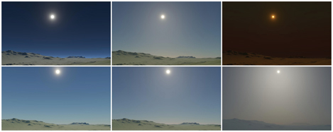
Figure 14.22. The two different types of atmospheric light scattering: Rayleigh only at the top and Mie with regular Rayleigh scattering at the bottom. From left to right: density of 0, regular density as described in [203], and exaggerated density. (Image courtesy of Frostbite, ©2018 Electronic Arts Inc. [743].)

The first physically based atmosphere model [1285] rendered the earth and its atmosphere from space, simulating single scattering. Similar results can by achieved using the method proposed by O’Neil [1333]. The earth can be rendered from ground to space using ray marching in a single-pass shader. Expensive ray marching to integrate Mie and Rayleigh scattering is done per vertex when rendering the sky dome. The visually high-frequency phase function is, however, evaluated in the pixel shader. This makes the appearance smooth and avoids revealing the sky geometry due to interpolation. It is also possible to achieve the same result by storing the scattering in a texture and to distribute the evaluation over several frames, accepting update latency for better performance [1871].

Analytical techniques use fitted mathematical models on measured sky radiance [1443] or reference images generated using expensive path tracing of light scattering in the atmosphere [778]. The set of input parameters is generally limited compared to those for a participating media material. For example, turbidity represents the contribution of particles resulting in Mie scattering, instead of σs $σ_{s}$ and σt $σ_{t}$ coefficients. Such a model presented by Preetham et al. [1443] evaluates the sky radiance in any direction using turbidity and sun elevation. It has been improved by adding support for spectral output, better directionality to the scattered radiance around the sun, and a new ground albedo input parameter [778]. Analytical sky models are fast to evaluate. They are, however, limited to ground views, and atmosphere parameters cannot be changed to simulate extra-terrestrial planets or achieve specific art-driven visuals.

Figure 14.23. Real-time rendering of the earth’s atmosphere from the ground (left) and from space (right) using a lookup table. (Image courtesy of Bruneton and Neyret [203].)

Another approach to rendering skies is to assume that the earth is perfectly spherical, with a layer of atmosphere around it composed of heterogeneous participating media. Extensive descriptions of the atmosphere’s composition are given by Bruneton and Neyret [203] as well as Hillaire [743]. Leveraging these facts, precomputed tables can be used to stored transmittance and scattering according to the current view altitude r, the cosine of the view vector angle relative to the zenith μv $μ_{v}$ , the cosine of the sun direction angle relative to the zenith μs $μ_{s}$ , and the cosine of the view vector angle relative to the sun direction in the azimuthal plane ν $ν$ . For instance, transmittance from the viewpoint to the atmosphere’s boundary can be parameterized by two parameters, r and μv $μ_{v}$ . During a precompute step, the transmittance can be integrated in the atmosphere and stored in a two-dimensional lookup table (LUT) texture Tlut $T_{} lut$ that can be sampled at runtime using the same parameterization. This texture can be used to apply atmosphere transmittance to sky elements such as the sun, stars, or other celestial bodies.

Considering scattering, Bruneton and Neyret [203] describe a way to store it in a four-dimensional LUT Slut $S_{} lut$ parameterized by all the parameters in the preceding paragraph. They also provide a way to evaluate multiple scattering of order n by iterating n times: (i) Evaluate the single-scattering table Slut $S_{} lut$ , (ii) evaluate Snlut $S_{}^{n} lut$ using Sn−1lut $S_{}^{n - 1} lut$ , and (iii) add the result to Slut $S_{} lut$ . Do (ii) and (iii) n−1 $n - 1$ times.

More details about the process, as well as source code, are provided by Bruneton and Neyret [203]. See Figure 14.23 for examples of the result. Bruneton and Neyret’s parameterization can sometimes exhibit visual artifacts at the horizon. Yusov [1957] has proposed an improved transformation. It is also possible to use an only three-dimensional LUT by ignoring ν $ν$ [419]. Using this scheme, the earth will not cast shadows in the atmosphere, which can be an acceptable trade-off. The advantage is that this LUT will be much smaller and less expensive to update and sample.

This last three-dimensional LUT approach is used by many Electronic Arts Frostbite real-time games, such as Need for Speed, Mirror’s Edge Catalyst, and FIFA [743]. In this case, artists can drive the physically based atmosphere parameters to reach a target sky visual and even simulate extra-terrestrial atmosphere. See Figure 14.24. The LUT has to be recomputed when atmosphere parameters are changed. To update these LUTs more efficiently, it is also possible to use a function that approximates the integral of the material in the atmosphere instead of ray-marching through it [1587]. The cost of updating the LUTs can be amortized down to 6% of the original by temporally distributing the evaluation of the LUTs and multiple scattering. This is achievable by updating only a sub-part of Snlut $S_{}^{n} lut$ for a given scattering order n, while interpolating the last two solved LUTs, accepting a few frames of latency. As another optimization, to avoid sampling the different LUTs multiple times per pixel, Mie and Rayleigh scattering are baked in voxels of a camera-frustum-mapped low-resolution volume texture. The visually high-frequency phase function is evaluated in the pixel shader in order to produce smooth scattering halos around the sun. Using this type of volume texture also permits applying aerial perspective per vertex on any transparent objects in the scene.

Figure 14.24. Real-time rendering using a fully parameterized model enables the simulation of the earth’s atmosphere (top) and the atmosphere of other planets, such as Mars’s blue sunset (bottom). (Top images courtesy of Bruneton and Neyret [203] and bottom images courtesy of Frostbite, ©2018 Electronic Arts Inc. [743].)

14.4.2. Clouds

Clouds are complex elements in the sky. They can look menacing when representing an incoming storm, or alternately appear discreet, epic, thin, or massive. Clouds change slowly, with both their large-scale shapes and small-scale details evolving over time. Large open-world games with weather and time-of-day changes are more complex cases that require dynamic cloud-rendering solutions. Different techniques can be used depending on the target performance and visual quality.

Figure 14.25. Different types of clouds on the earth. (Image courtesy of Valentin de Bruyn.)

Clouds are made of water droplets, featuring high-scattering coefficients and complex phase functions that result in a specific look. They are often simulated using participating media, as described in Section 14.1, and their materials have been measured as having a high single-scattering albedo ρ=1 $ρ = 1$ and extinction coefficients σt $σ_{t}$ in the range [0.04, 0.06] for stratus (low-level horizontal cloud layers) and [0.05, 0.12] for cumulus [743] (isolated low-level cotton-like fluffy clouds). See Figure 14.25. Given the fact that ρ $ρ$ is close to 1, σs=σt $σ_{s} = σ_{t}$ can be assumed.

A classic approach to cloud rendering is to use a single panoramic texture composited over the sky using alpha blending. This is convenient when rendering a static sky. Guerrette [620] presents a visual flow technique that gives the illusion of cloud motion in the sky affected by a global wind direction. This is an efficient method that improves over the use of a static set of panoramic cloud textures. However, it will not be able to represent any change to the cloud shapes and lighting.

Clouds as Particles

Harris renders clouds as volumes of particles and impostors [670]. See Section 13.6.2 and Figure 13.9 on page 557.

Another particle-based cloud rendering method is presented by Yusov [1959]. He uses rendering primitives that are called volume particles. Each of these is represented by a four-dimensional LUT, allowing retrieval of scattered light and transmittance on the view-facing quad particle as a function of the sun light and view directions. See Figure 14.26.

This approach is well suited to render stratocumulus clouds. See Figure 14.25.

When rendering clouds as particles, discretization and popping artifacts can often be seen, especially when rotating around clouds. These problems can be avoided by using volume-aware blending. This ability is made possible by using a GPU feature called rasterizer order views (Section ). Volume-aware blending enables the synchronization of pixel shader operations on resources per primitive, allowing deterministic custom blending operations. The closest n particles’ depth layers are kept in a buffer at the same resolution as the render target into which we render. This buffer is read and used to blend the currently rendered particle by taking into account intersection depth, then finally written out again for the next particle to be rendered. The result is visible in Figure 14.27.

Figure 14.26. Clouds rendered as volumes of particles. (Image courtesy of Egor Yusov [1959].)

Clouds as Participating Media

Considering clouds as isolated elements, Bouthors et al. [184] represent a cloud with two components: a mesh, showing its overall shape, and a hypertexture [1371], adding high-frequency details under the mesh surface up to a certain depth inside the cloud. Using this representation, a cloud edge can be finely ray-marched in order to gather details, while the inner part can be considered homogeneous. Radiance is integrated while ray marching the cloud structure, and different algorithms are used to gather scattered radiance according to scattering order. Single scattering is integrated using an analytical approach described in Section 14.1. Multiple scattering evaluation is accelerated using offline precomputed transfer tables from disk-shaped light collectors positioned at the cloud’s surface. The final result is of high visual quality, as shown in Figure 14.28.

Figure 14.27. On the left, cloud particles rendered the usual way. On the right, particles rendered with volume-aware blending. (Images courtesy of Egor Yusov [1959].)

Figure 14.28. Clouds rendered using meshes and hypertextures. (Image courtesy of Bouthors et al. [184].)

Instead of rendering clouds as isolated elements, it is possible to model them as a layer of participating media in the atmosphere. Relying on ray marching, Schneider and Vos presented an efficient method to render clouds in this way [1572].

With only a few parameters, it is possible to render complex, animated, and detailed cloud shapes under dynamic time-of-day lighting conditions, as seen in Figure 14.29. The layer is built using two levels of procedural noise. The first level gives the cloud its base shape. The second level adds details by eroding this shape. In this case, a mix of Perlin [1373] and Worley [1907] noise is reported to be a good representation of the cauliflower-like shape of cumulus and similar clouds. Source code and tools to generate such textures have been shared publicly [743,1572]. Lighting is achieved by integrating scattered light from the sun using samples distributed in the cloud layer along the view ray.

Figure 14.29. Clouds rendered using a ray-marched cloud layer using Perlin-Worley noise, and featuring dynamic volumetric lighting and shadowing. (Results by Schneider and Vos [1572], copyright ©2017 Guerrilla Games.)

Volumetric shadowing can be achieved by evaluating the transmittance for a few samples within the layer, testing toward the sun [743,1572] as a secondary ray marching. It is possible to sample the lower mipmap levels of the noise textures for these shadow samples in order to achieve better performance and to smooth out artifacts that can become visible when using only a few samples. An alternative approach to avoid secondary ray marching per sample is to encode the transmittance curve from the sun once per frame in textures, using one of the many techniques available ( ). For instance, the game Final Fantasy XV [416] uses transmittance function mapping [341].

Rendering clouds at high resolution with ray marching can become expensive if we want to capture every little detail. To achieve better performance, it is possible to render clouds at a low resolution. One approach is to update only a single pixel within each 4×4 $4 \times 4$ block and reproject the previous frame data to fill up the rest [1572]. Hillaire [743] proposes a variation that always renders at a fixed lower resolution and adds noise on the view ray marching start position. The previous frame result can be reprojected and combined with the new frame using an exponential moving average [862]. This approach renders at lower resolution but can converge faster.

Figure 14.30. Clouds rendered using a ray-marched cloud layer with dynamic lighting and shadowing using a physically based representation of participating media as described by Hillaire [743]. (Images courtesy of Sören Hesse (top) and Ben McGrath (bottom) from BioWare, ©2018 Electronic Arts Inc.)

Clouds’ phase functions are complex [184]. Here we present two methods that can be used to evaluate them in real time. It is possible to encode the function as a texture and sample it based on θ $θ$ . If doing so requires too much memory bandwidth, it is possible to approximate the function by combining two Henyey-Greenstein phase functions from Section 14.1.6 [743] as

(14.17)

p dual (θ, g 0, g 1, w) = p dual 0 + w (p dual 1 - p dual 0),

$\begin{matrix} p_{} dual (θ, g_{0}, g_{1}, w) = p_{{dual}_{0}} + w (p_{{dual}_{1}} - p_{{dual}_{0}}), \end{matrix}$

where the two main scattering eccentricities g0 $g_{0}$ and g1 $g_{1}$ , as well as the blend factor w, can be authored by an artist. This is important in representing both the main forward and backward scattering directions, revealing details in clouds when looking both away from and toward the light source, e.g., the sun or moon. See Figure 14.30.

There are different ways to approximate scattered light from ambient lighting in clouds. A straightforward solution is to use a single radiance input uniformly integrated from a render of the sky into a cube map texture. A bottom-up, dark-to-light gradient can also be used to scale the ambient lighting to approximate occlusion from clouds themselves. It is also possible to separate this input radiance as bottom and top, e.g., ground and sky [416]. Then ambient scattering can analytically be integrated for both contributions, assuming constant media density within thecloud layer [1149].

Multiple Scattering Approximation

Clouds’ bright and white look is the result of light scattering multiple times within them. Without multiple scattering, thick clouds would mostly be lit at the edge of their volumes, and they would appear dark everywhere else. Multiple scattering is a key component for clouds to not look smoky or murky. It is excessively expensive to evaluate multiple scattering using path tracing. A way to approximate this phenomenon when ray marching has been proposed by Wrenninge [1909]. It integrates o octaves of scattering and sums them as

(14.18)

L m u l t i s c a t (x, v) = \sum o - 1 n = 0 L scat (x, v),

$\begin{matrix} L_{m u l t i s c a t} (x, v) = \sum_{n = 0}^{o - 1} L_{scat} (x, v), \end{matrix}$

where the following substitutions are made when evaluating Lscat $L_{scat}$ (for instance, using σ′s $σ_{s}^{'}$ instead of σs $σ_{s}$ ): σ′s=σsan $σ_{s}^{'} = σ_{s} a^{n}$ , σ′e=σebn $σ_{e}^{'} = σ_{e} b^{n}$ , and p′(θ)=p(θcn) $p^{'} (θ) = p (θ c^{n})$ ,

where a, b, and c are user-control parameters in [0, 1] that will let the light punch through the participating media. Clouds look softer when these values are closer to 0. In order to make sure this technique is energy-conserving when evaluating Lmultiscat(x,v) $L_{m u l t i s c a t} (x, v)$ , we must ensure that a≤b $a \leq b$ . Otherwise, more light can scatter, because the equation σt=σa+σs $σ_{t} = σ_{a} + σ_{s}$ would not be respected, as σs $σ_{s}$ could end up being larger than σt $σ_{t}$ . The advantage of this solution is that it can integrate the scattered light for each of the different octaves on the fly while ray marching. The visual improvement is presented in Figure 14.31. The drawback is that it does a poor job at complex multiple scattering behavior when light could scatter in any direction. However, the look of the clouds is improved, and this method allows lighting artists to easily control the visuals with a few parameters and express their vision, thanks to a wider range of achievable results. With this approach, light can punch through the medium and reveal more internal details.

Figure 14.31. Clouds rendered using Equation 14.18 as an approximation to multiple scattering. From left to right, n is set to 1, 2, and 3. This enable the sun light to punch through the clouds in a believable fashion. (Image courtesy of Frostbite, ©2018 Electronic Arts Inc. [743].)

Clouds and Atmosphere Interactions

When rendering a scene with clouds, it is important to take into account interactions with atmospheric scattering for the sake of visual coherency. See Figure 14.32.

Since clouds are large-scale elements, atmospheric scattering should be applied to them. It is possible to evaluate the atmospheric scattering presented in Section 14.4.1 for each sample taken through the cloud layer, but doing so quickly becomes expensive. Instead it is possible to apply the atmospheric scattering on the cloud according to a single depth representing the mean cloud depth and transmittance [743].

Figure 14.32. Clouds entirely covering the sky are rendered by taking into account the atmosphere [743]. Left: without atmospheric scattering applied on the clouds, leading to incoherent visuals. Middle: with atmospheric scattering, but the environment appears too bright without shadowing. Right: with clouds occluding the sky, thus affecting the light scattering in the atmosphere and resulting in coherent visuals. (Image courtesy of Frostbite, ©2018 Electronic Arts Inc. [743].)

If cloud coverage is increased to simulate rainy weather, sunlight scattering in the atmosphere should be reduced under the cloud layer. Only light scattered through the clouds should scatter in the atmosphere under them. The illumination can be modified by reducing the sky’s lighting contribution to the aerial perspective and adding scattered light back into the atmosphere [743]. The visual improvement is shown in Figure 14.32.

To conclude, cloud rendering can be achieved with advanced physically based material representation and lighting. Realistic cloud shapes and details can be achieved by using procedural noise. Finally, as presented in this section, it is also important to keep in mind the big picture, such as interactions of clouds with the sky, in order to achieve coherent visual results.

14.5 Translucent Surfaces

Translucent surfaces typically refer to materials having a high absorption together with low scattering coefficients. Such materials include glass, water, or the wine shown in Figure 14.2 on page 592. In addition, this section will also discuss translucent glass with a rough surface. These topics are also covered in detail in many publications [1182,1185,1413].

14.5.1. Coverage and Transmittance

As discussed in Section 5.5, a transparent surface can be treated as having a coverage represented by α $α$ , e.g., opaque fabric or tissue fibers hiding a percentage of what lies behind. For glass and other materials, we want to compute the translucency, where a solid volume lets a percentage of each light wavelength pass through, acting as a filter over the background as a function of transmittance Tr $T_{r}$ (Section 14.1.2). With the output color co $c_{o}$ , the surface radiance cs $c_{s}$ , and the background color cb $c_{b}$ , the blending operation for a transparency-as-coverage surface is

(14.19)

c o = α c s + (1 - α) c b .

$\begin{matrix} c_{o} = α c_{s} + (1 - α) c_{b} . \end{matrix}$

In the case of a translucent surface, the blending operation will be

(14.20)

c o = c s + T r c b,

$\begin{matrix} c_{o} = c_{s} + T_{r} c_{b}, \end{matrix}$

where cs $c_{s}$ contains the specular reflection of the solid surface, i.e., glass or a gel. Note that Tr $T_{r}$ is a three-valued transmittance color vector. To achieve colored translucency, one can use the dual-source color blending feature of any modern graphics API in order to specify these two output colors to blend with the target buffer color cb $c_{b}$ . Drobot [386] presents the different blending operations that can be used depending on whether, for a given surface, reflection and transmittance are colored or not.

In the general case, it is possible to use a common blending operation for coverage and translucency specified together [1185]. The blend function to use in this case is

(14.21)

c o = α (c s + T r c b) + (1 - α) c b .

$\begin{matrix} c_{o} = α (c_{s} + T_{r} c_{b}) + (1 - α) c_{b} . \end{matrix}$

When the thickness varies, the amount of light transmitted can be computed using Equation 14.3, which can be simplified to

(14.22)

T r = e - σ t d,

$\begin{matrix} T_{r} = e^{- σ_{t} d}, \end{matrix}$

where d is the distance traveled through the material volume. The physical extinction parameter σt $σ_{t}$ represents the rate at which light drops off as it travels through the medium. For intuitive authoring by artists, Bavoil [115] sets the target color tc $t_{c}$ to be the amount of transmittance at some given distance d. Then extinction σt $σ_{t}$ can be recovered as

(14.23)

σ t = - log ( t c ) d .

$\begin{matrix} σ_{t} = \frac{- log (t_{c})}{d} . \end{matrix}$

For example, with target transmittance color tc=(0.3,0.7,0.1) $t_{c} = (0.3, 0.7, 0.1)$ and distance d=4.0 $d = 4.0$ meters, we recover

(14.24)

σ t = 1 4 (- log 0.3, - log 0.7, - log 0.1) = (0.3010, 0.0892, 0.5756) .

$\begin{matrix} σ_{t} = \frac{1}{4} (- log 0.3, - log 0.7, - log 0.1) = (0.3010, 0.0892, 0.5756) . \end{matrix}$

Note that a transmittance of 0 needs to be handled as a special case. A solution is to subtract a small epsilon, e.g., 0.000001, from each component of Tr $T_{r}$ . The effect of color filtering is shown in Figure 14.33.

Figure 14.33. Translucency with different absorption factors through multiple layers of a mesh [115]. (Images courtesy of Louis Bavoil [115].)

In the case of an empty shell mesh whose surface consists of a single thin layer of translucent material, the background color should be occluded as a function of the path length d that the light has traveled within the medium. So, viewing such as surface along its normal or tangentially will result in a different amount of background occlusion as a function of its thickness t, because the path length changes with angle. Drobot [386] proposes such an approach where the transmittance Tr $T_{r}$ is evaluated as

(14.25)

T r = e - σ t d, where d = t max ( 0.001 , n \cdot v ) .

$\begin{matrix} T_{r} = e^{- σ_{t} d}, where d = \frac{t}{max (0.001, n \cdot v)} . \end{matrix}$

Figure 14.34 shows the result. See Section for more details about thin-film and multi-layer surfaces.

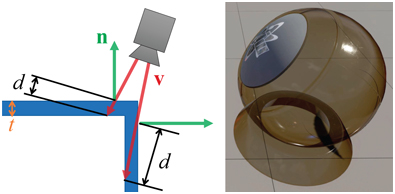
Figure 14.34. Colored transmittance computed from the distance d a view ray v $v$ has traveled within a transparent surface of thickness t. (Right image courtesy of Activision Publishing, Inc. 2018.)

In the case of solid translucent meshes, computing the actual distance that a ray travels through a transmitting medium can be done in many ways. A common method is to first render the surface where the view ray exits the volume. This surface could be the backface of a crystal ball, or could be the sea floor (i.e., where the water ends). The depth or location of this surface is stored. Then the volume’s surface is rendered. The stored exit depth is accessed in the shader, and the distance between it and the current pixel surface is computed. This distance is then used to compute the transmittance to apply over the background.

This method works if it is guaranteed that the volume is closed and convex, i.e., it has one entry and one exit point per pixel, as with a crystal ball. Our seabed example also works because once we exit the water we encounter an opaque surface, so further transmittance will not occur. For more elaborate models, e.g., a glass sculpture or other object with concavities, two or more separate spans may absorb incoming light. Using depth peeling, as discussed in Section 5.5, we can render the volume surfaces in precise back-to-front order. As each frontface is rendered, the distance through the volume is computed and used to compute transmittance. Applying each of these in turn gives the proper final transmittance. Note that if all volumes are made of the same material at the same concentration, the transmittance could be computed once at the end using the summed distances, if the surface has no reflective component. A-buffer or K-buffer methods directly storing object fragments in a single pass can also be used for more efficiency on recent GPUs [115,230]. Such an example of multi-layer transmittance is shown in Figure 14.33.

In the case of large-scale sea water, the scene depth buffer can be directly used as a representation of the backface seabed. When rendering transparent surfaces, one must consider the Fresnel effect, as described in Section 9.5. Most transmitting media have an index of refraction significantly higher than that of air. At glancing angles, all the light will bounce back from the interface, and none will be transmitted. Figure 14.35 shows this effect, where underwater objects are visible when looking directly into the water, but looking farther out, at a grazing angle, the water surface mostly hides what is beneath the waves. Several articles explain handling reflection, absorption, and refraction for large bodies of water [261,977].

Figure 14.35. Water rendered taking into account the transmittance and reflectance effects. Looking down, we can see into the water with a light blue tint since transmittance is high and blue. Near the horizon the seabed becomes less visible due to a lower transmittance (because light has to travel far into the water volume) and reflection increasing at the expense of transmission, due to the Fresnel effect. (Image from “Crysis,” courtesy of Crytek.)

14.5.2. Refraction

For transmittance we assume that the incoming light comes from directly beyond the mesh volume, in a straight line. This is a reasonable assumption when the front and back surfaces of the mesh are parallel and the thickness is not great, e.g., for a pane of glass. For other transparent media, the index of refraction plays an important role. Snell’s law, which describes how light changes direction when a mesh’s surface is encountered, is described in Section 9.5.

Figure 14.36. Refracted and transmitted radiance as a function of incident angle θi $θ_{i}$ and transmission angle θt $θ_{t}$ .

Due to conservation of energy, any light not reflected is transmitted, so the proportion of transmitted flux to incoming flux is 1−f $1 - f$ , where f is the amount of reflected light. The proportion of transmitted-to-incident radiance, however, is different. Due to differences in projected area and solid angle between the incident and transmitted rays, the radiance relationship is

(14.26)

L t = (1 - F (θ i)) sin 2 θ i sin 2 θ t L i .

$\begin{matrix} L_{t} = (1 - F (θ_{i})) \frac{{sin}^{2} θ_{i}}{{sin}^{2} θ_{t}} L_{i} . \end{matrix}$

This behavior is illustrated in Figure 14.36. Snell’s law combined with Equation 14.26 yields a different form for transmitted radiance:

(14.27)

L t = (1 - F (θ i)) n 2 2 n 2 1 L i .

$\begin{matrix} L_{t} = (1 - F (θ_{i})) \frac{n_{2}^{2}}{n_{1}^{2}} L_{i} . \end{matrix}$

Bec [123] presents an efficient method to compute the refraction vector. For readability (because n is traditionally used for the index of refraction in Snell’s equation), we define N $N$ as the surface normal and l $l$ as the direction to the light:

(14.28)

t = (w - k) N - n l,

$\begin{matrix} t = (w - k) N - n l, \end{matrix}$

where n=n1/n2 $n = n_{1} / n_{2}$ is the relative index of refraction, and

(14.29)

w k = n (l \cdot N), = 1 + (w - n) (w + n) - - - - - - - - - - - - - - - - \sqrt .

$\begin{matrix} \begin{matrix} w & = n (l \cdot N), \\ k & = \sqrt{1 + (w - n) (w + n)} . \end{matrix} \end{matrix}$

The resulting refraction vector t $t$ is returned normalized. Water has an index of refraction of approximately 1.33, glass typically around 1.5, and air effectively 1.0.

The index of refraction varies with wavelength. That is, a transparent medium will bend each color of light at a different angle. This phenomenon is called dispersion, and explains why prisms spread out white light into a rainbow-colored light cone and why rainbows occur. Dispersion can cause a problem in lenses, termed chromatic aberration. In photography, this phenomenon is called purple fringing, and can be particularly noticeable along high contrast edges in daylight. In computer graphics we normally ignore this effect, as it is usually an artifact to be avoided. Additional computation is needed to properly simulate the effect, as each light ray entering a transparent surface generates a set of light rays that must then be tracked. As such, normally a single refracted ray is used. It is worthwhile to note that some virtual reality renderers apply an inverse chromatic aberration transform, to compensate for the headset’s lenses [1423,1823].

A general way to give an impression of refraction is to generate a cubic environment map (EM) from the refracting object’s position.

When this object is then rendered, the EM can be accessed by using the refraction direction computed for the frontfacing surfaces. An example is shown in Figure 14.37.

Figure 14.37. Left: refraction by glass angels of a cubic environment map, with the map itself used as a skybox background. Right: reflection and refraction by a glass ball with chromatic aberration. (Left image from the three.js example webgl_materials_cube map_refraction [218], Lucy model from the Stanford 3D scanning repository, texture by Humus. Right image courtesy of Lee Stemkoski [1696].)

Instead of using an EM, Sousa [1675] proposes a screen-space approach. First, the scene is rendered as usual without any refractive objects into a scene texture s $s$ . Second, refractive objects are rendered into the alpha channel of s $s$ that was first cleared to 1. If pixels pass the depth test, a value of 0 is written. Finally, refractive objects are rendered fully, and in the pixel shader s $s$ is sampled according to pixel position on the screen with a perturbed offset coming from, for instance, the scaled surface normal tangent xy-components, simulating refraction. In this context, the color of the perturbed samples is taken into account only if α=0 $α = 0$ . This test is done to avoid using samples from surfaces that are in front of the refractive object and so having their colors pulled in as if they were behind it. Note that instead of setting α=0 $α = 0$ , the scene depth map could be used to compare the pixel shader depth against the perturbed scene sample’s depth [294]. If the center pixel is farther away, the offset sample is closer; it is then ignored and replaced by the regular scene sample as if there was no refraction.

These techniques give the impression of refraction, but bear little resemblance to physical reality. The ray gets redirected when it enters the transparent solid, but the ray is never bent a second time, when it is supposed to leave the object. This exit interface never comes into play. This flaw sometimes does not matter, because human eyes are forgiving for what the correct appearance should be [1185].

Figure 14.38. Transparent glasses at the bottom of the image features roughness-based background scattering. Elements behind the glass appear more or less blurred, simulating the spreading of refracted rays. (Image courtesy of Frostbite, ©2018 Electronic Arts Inc.)

Many games feature refraction through a single layer. For rough refractive surfaces, it is important to blur the background according to material roughness, to simulate the spreading of refracted ray directions caused by the distribution of microgeometry normals. In the game DOOM (2016) [1682], the scene is first rendered as usual. It is then downsampled to half resolution and further down to four mipmap levels. Each mipmap level is downsampled according to a Gaussian blur mimicking a GGX BRDF lobe. In the final step, refracting meshes are rendered over the full-resolution scene [294]. The background is composited behind the surfaces by sampling the scene’s mipmapped texture and mapping the material roughness to the mipmap level. The rougher the surface, the blurrier the background. Using a general material representation, the same approach is proposed by Drobot [386]. A similar technique is also used within a unified transparency framework from McGuire and Mara [1185]. In this case, a Gaussian point-spread function is used to sample the background in a single pass. See Figure 14.38.

It is also possible to handle the more complex case of refraction through multiple layers. Each layer can be rendered with the depths and normals stored in textures. A procedure in the spirit of relief mapping (Section 6.8.1) can then be used to trace rays through the layers. Stored depths are treated as a heightfield that each ray walks until an intersection is found. Oliveira and Brauwers [1326] present such a framework to handle refraction through backfaces of meshes. Furthermore, nearby opaque objects can be converted into color and depth maps, providing a last opaque layer [1927]. A limitation of all these image-space refraction schemes is that what is outside of the screen’s boundaries cannot refract or be refracted.

14.5.3. Caustics and Shadows

Evaluating shadows and caustics resulting from refracted and attenuated light is a complex task. In a non-real-time context, multiple methods, such as bidirectional path tracing or photon mapping [822,1413], are available to achieve this goal. Luckily, many methods offer approximations of such phenomenon in real time.

Figure 14.39. Real-world caustics from reflection and refraction.

Caustics are the visual result of light being diverged from its straight path, for instance by a glass or water surface. The result is that the light will be defocused from some areas, creating shadows, and focused in some others, where ray paths become more dense, resulting in stronger incident lighting. Such paths depend on the curved surface that the light encounters. A classic example for reflection is the cardioid caustic seen inside a coffee mug. Refractive caustics are more noticeable, e.g., light focused through a crystal ornament, a lens, or a glass of water. See Figure 14.39. Caustics can also be created due to light being reflected and refracted by a curved water surface, both above and below. When converging, light will concentrate on opaque surfaces and generate caustics. When under the water surface, converging light paths will become visible within the water volume. This will result in well-known light shafts from photons scattering through water particles. Caustics are a separate factor beyond the light reduction coming from Fresnel interaction at the volume’s boundary and the transmittance when traveling through it.

Figure 14.40. Demo of caustic effects in water. (Image from WebGL Water demo courtesy of Evan Wallace [1831].)

In order to generate caustics from water surfaces, one may apply an animated texture of caustics generated offline as a light map applied on a surface, potentially added on top of the usual light map. Many games have taken advantage of such an approach, such as Crysis 3 running on CryEngine [1591]. Water areas in a level are authored using water volumes. The top surface of the volume can be animated using a bump map texture animation or a physical simulation. The normal resulting from the bump map can be used, when vertically projected above and under the water surface, to generate caustics from their orientation mapped to a radiance contribution. Distance attenuation is controlled using an artist-authored height-based maximum influence distance. The water surface can also be simulated, reacting to object motion in the world and thus generating caustic events matching what is occurring in the environment. An example is shown in Figure 14.40.

When underwater, the same animated water surface can also be used for caustics within the water medium. Lanza [977] propose a two-step method to generate light shafts. First, light positions and refraction directions are rendered from the light’s point of view and saved into a texture. Lines can then be rasterized starting from the water surface and extending in the refraction direction in the view. They are accumulated with additive blending, and a final post-process blur can be used to blur out the result in order to mask the low number of lines.

Wyman [1928,1929] presents an image-space technique for caustic rendering. It works by first evaluating photon positions and incident directions after refraction through transparent objects’ front- and backfaces. This is achieved by using the background refraction technique [1927] presented in Section 14.5.2. However, instead of storing refracted radiance, textures are used to store the scene intersection position, post-refraction incident direction, and transmittance due to the Fresnel effect. Each texel stores a photon that can then be splatted with the correct intensity back into the view. To achieve this goal there are two possibilities: Splat photons as quads in view space or in light space, with Gaussian attenuation. One result is shown in Figure 14.41. McGuire and Mara [1185] proposed a simpler approach to caustic-like shadows by varying transmittance based on the transparent surface’s normal, transmitting more if perpendicular to the incident surface and less otherwise, due to the Fresnel effect. Other volumetric shadow techniques are described in Section 7.8.

Figure 14.41. On the left, the Buddha refracts both nearby objects and the surrounding skybox [1927]. On the right, caustics are generated via hierarchical maps similar in nature to shadow maps [1929]. (Images courtesy of Chris Wyman, University of Iowa.)

14.6 Subsurface Scattering

Subsurface scattering is a complex phenomenon found in solid materials having high scattering coefficients (see Section 9.1.4 for more details). Such materials include wax, human skin, and milk, as seen in Figure 14.2 on page 592.

General light scattering theory has been explained in Section 14.1. In some cases, the scale of scattering is relatively small, as for media with a high optical depth, such as human skin. Scattered light is re-emitted from the surface close to its original point of entry. This shift in location means that subsurface scattering cannot be modeled with a BRDF (Section 9.9). That is, when the scattering occurs over a distance larger than a pixel, its more global nature is apparent. Special methods must be used to render such effects.

Figure 14.42. Light scattering through an object. Initially the light transmitted into the object travels in the refraction direction, but scattering causes it to change direction repeatedly until it leaves the material. The length of each path through the material determines the percentage of light lost to absorption.

Figure 14.42 shows light being scattered through an object. Scattering causes incoming light to take many different paths. Since it is impractical to simulate each photon separately (even for offline rendering), the problem must be solved probabilistically, by integrating over possible paths or by approximating such an integral. Besides scattering, light traveling through the material also undergoes absorption.

One important factor that distinguishes the various light paths shown in Figure 14.42 is the number of scattering events. For some paths, the light leaves the material after being scattered once; for others, the light is scattered twice, three times, or more. Scattering paths are commonly grouped as single scattering and multiple scattering. Different rendering techniques are often used for each group. For some materials, single scattering is a relatively weak part of the total effect, and multiple scattering predominates, e.g., skin. For these reasons, many subsurface scattering rendering techniques focus on simulating multiple scattering. In this section we present several techniques to approximate subsurface scattering.

14.6.1. Wrap Lighting

Perhaps the simplest of the subsurface scattering methods is wrap lighting [193]. This technique was discussed on page 382 as an approximation of area light sources. When used to approximate subsurface scattering, we can add a color shift [586]. This accounts for the partial absorption of light traveling through the material. For example, when rendering skin, a red color shift could be applied.

When used in this way, wrap lighting attempts to model the effect of multiple scattering on the shading of curved surfaces. The “leakage” of light from adjacent points into the currently shaded point softens the transition area from light to dark where the surface curves away from the light source. Kolchin [922] points out that this effect depends on surface curvature, and he derives a physically based version. Although the derived expression is somewhat expensive to evaluate, the ideas behind it are useful.

14.6.2. Normal Blurring

Stam [1686] points out that multiple scattering can be modeled as a diffusion process. Jensen et al. [823] further develop this idea to derive an analytical bidirectional surface scattering distribution function (BSSRDF) model. The BSSRDF is a generalization of the BRDF for the case of global subsurface scattering [1277]. The diffusion process has a spatial blurring effect on the outgoing radiance.

This blurring is applied to only the diffuse reflectance. Specular reflectance occurs at the material surface and is unaffected by subsurface scattering. Since normal maps often encode small-scale variation, a useful trick for subsurface scattering is to apply normal maps to only the specular reflectance [569]. The smooth, unperturbed normal is used for the diffuse reflectance. Since there is no added cost, it is often worthwhile to apply this technique when using other subsurface scattering methods.

For many materials, multiple scattering occurs over a relatively small distance. Skin is an important example, where most scattering takes place over a distance of a few millimeters. For such materials, the technique of not perturbing the diffuse shading normal may be sufficient by itself. Ma et al. [1095] extend this method, based on measured data. They determined the reflected light from scattering objects and found that, while the specular reflectance is based on the geometric surface normals, subsurface scattering makes diffuse reflectance behave as if it uses blurred surface normals. Furthermore, the amount of blurring can vary over the visible spectrum. They propose a real-time shading technique using independently acquired normal maps for the specular reflectance and for the R, G, and B channels of the diffuse reflectance [245]. Using different normal maps for each channel will then result in color bleeding. Since these diffuse normal maps typically resemble blurred versions of the specular map, it is straightforward to modify this technique to use a single normal map, while adjusting the mipmap level, but at the cost of losing the color shift since the normal is the same for each channel.

14.6.3. Pre-Integrated Skin Shading

Combining the idea of wrap lighting and normal blurring, Penner [1369] proposes a pre-integrated skin shading solution.

Scattering and transmittance are integrated and stored in a two-dimensional lookup table. The LUT’s first axis is indexed based on n⋅l $n \cdot l$ . The second axis is indexed based on 1/r=||∂n/∂p|| $1 / r = ||\partial n / \partial p||$ , representing the surface curvature. The higher the curvature, the greater the impact on the transmitted and scattered color. Because curvature is constant per triangle, these values must be baked and smoothed offline.

To handle the effect of subsurface scattering on small surface details, Penner modifies the technique by Ma et al. [1095], which was discussed in the previous section. Instead of acquiring separate normal maps for the R, G, and B diffuse reflectance, Penner generates them by blurring the original normal map according to the diffusion profile of the subsurface material for each color channel. Since using four separate normal maps is memory intensive, as an optimization he uses a single smoothed normal map that is blended with the vertex normal for each color channel.

This technique will ignore light diffusion across shadow boundaries, since by default it only relies on curvature. To get the scattering profile to span through shadow boundaries, the shadow penumbra profile can be used to bias the LUT coordinates. Thus, this fast technique is able to approximate the high-quality method presented in the next section [345].

14.6.4. Texture-Space Diffusion

Blurring the diffuse normals accounts for some visual effects of multiple scattering, but not for others, such as softened shadow edges. The concept of texture-space diffusion can be used to address these limitations. This idea was introduced by Lensch et al. [1032] as part of a different technique, but the version presented by Borshukov and Lewis [178,179] has been the most influential. They formalize the idea of multiple scattering as a blurring process. First, the surface irradiance (diffuse lighting) is rendered into a texture. This is done by using texture coordinates as positions for rasterization. The real positions are interpolated separately for use in shading. This texture is blurred and then used for diffuse shading when rendering. The shape and size of the filter depends on the material and on the wavelength. For example, for skin, the R channel is filtered with a wider filter than G or B, causing reddening near shadow edges. The correct filter for simulating subsurface scattering in most materials has a narrow spike in the center and a wide, shallow base. This technique was first presented for use in offline rendering, but real-time GPU implementations were soon proposed by researchers at NVIDIA [345,586] and ATI [568,569,803,1541].

The presentation by d’Eon and Luebke [345] represents one of the most complete treatments of this technique, including support for complex filters mimicking the effect of multi-layer subsurface structure. Donner and Jensen [369] show that such structures produce the most realistic skin renderings. The full NVIDIA skin rendering system presented by d’Eon and Luebke produces excellent results (see Figure 14.43 for an example), but is quite expensive, requiring a large number of blurring passes. However, it can easily be scaled back to increase performance.

Figure 14.43. Texture-space multi-layer diffusion. Six different blurs are combined using RGB weights. The final image is the result of this linear combination, plus a specular term. (Images courtesy of NVIDIA Corporation [345].)

Instead of applying multiple Gaussian passes, Hable [631] presents a single 12-sample kernel. The filter can be applied either in texture space as a preprocess or in the pixel shader when rasterizing the mesh on screen. This makes face rendering much faster at the cost of some realism. When close up, the low amount of sampling can become visible as bands of color. However, from a moderate distance, the difference in quality is not noticeable.

14.6.5. Screen-Space Diffusion

Rendering a light map and blurring it for all the meshes in a scene can quickly become expensive, both computationally and memory-wise. Furthermore, the meshes need to be rendered twice, once in the light map and once in the view, and the light map needs to have a reasonable resolution to be able to represent subsurface scattering from small-scale details.

To counter these issues, Jimenez proposed a screen-space approach [831]. First, the scene is rendered as usual and meshes requiring subsurface scattering, e.g., human faces, will be noted in the stencil buffer. Then a two-pass screen-space process is applied on the stored radiance to simulate subsurface scattering, using the stencil test to apply the expensive algorithm only where it is needed, in pixels containing translucent material. The additional passes apply the two one-dimensional and bilateral blur kernels, horizontally and vertically. The colored blur kernel is separable, but it cannot be applied in a fully separable fashion for two reasons. First, linear view depth must be taken into account to stretch the blur to a correct width, according to surface distance. Second, bilateral filtering avoids light leaking from materials at different depths, i.e., between surfaces that should not interact. In addition, the normal orientation must be taken into account for the blur filter to be applied not only in screen space but tangentially to the surface. In the end, this makes the separability of the blur kernel an approximation, but still a high-quality one. Later, an improved separable filter was proposed [833]. Being dependent on the material area on screen, this algorithm is expensive for close-ups on faces. However, this cost is justifiable, since high quality in these areas is just what is desired. This algorithm is especially valuable when a scene is composed of many characters, since they will all be processed at the same time. See Figure 14.44.

Figure 14.44. High-quality render of scanned model faces. Screen-space subsurface scattering makes it possible to render realistic human skin material on many characters with a single post-process. (Left image: render courtesy of Jorge Jimenez and Diego Gutierrez, Universidad de Zaragoza. Scan courtesy of XYZRGB Inc. Right image: render courtesy of Jorge Jimenez et al., Activision Publishing, Inc., 2013 and Universidad de Zaragoza. Scan courtesy of Lee Perry-Smith, Infinite-Realities [831].)

To further optimize the process, the linear depth can be stored in the alpha channel of the scene texture. The one-dimensional blur relies on a low number of samples, so undersampling can be visible on faces close up. To avoid this issue, the kernel can be rotated per pixel, which will hide ghosting artifacts with noise [833]. The visibility of this noise can be significantly reduced by using temporal antialiasing (Section ).

When implementing screen-space diffusion, care must be taken to blur only irradiance and not the diffuse albedo or specular lighting. One way to achieve this goal is to render irradiance and specular lighting into separate screen-space buffers. If deferred shading (Section ) is used, then a buffer with diffuse albedo is already available. To reduce memory bandwidth, Gallagher and Mittring [512] propose storing irradiance and specular lighting in a single buffer, using a checkerboard pattern. After the irradiance has been blurred, the final image is composited by multiplying the diffuse albedo with the blurred irradiance and adding the specular lighting on top.

Within this screen-space framework, it is also possible to render large-scale subsurface scattering phenomena, such as the light traveling through the nose or ears. When rendering the mesh diffuse lighting, the technique presented by Jimenez et al. [827] also adds the subsurface transmission from backface contributions by sampling the incoming light from the opposite side using the negated surface normal −n $- n$ . The result is modulated by a transmittance value estimated using the depth recovered by sampling a traditional shadow map rendered from the light’s point of view, similarly to the method by Dachsbacher and Stamminger [320] described in the next section. To represent forward scattering in a cone, the shadow map can be sampled multiple times. In order to use a low sample count per pixel to reduce the cost of rendering, it is possible to take two shadow samples with a randomized offset or rotation per pixel. Doing so will result in much unwanted visual noise. Thankfully, this noise can automatically be filtered out for free by the screen-space subsurface blur kernel required to achieve the translucent subsurface light diffusion. It is thus possible to render high-quality translucency effects simulating forward light scattering in a cone through the thin parts of a face with only one extra depth-map sample per light source.

14.6.6. Depth-Map Techniques

The techniques discussed so far model light scattering over relatively small distances, e.g., skin. Other techniques are needed for materials exhibiting large-scale scattering, such as light traveling through a hand. Many of these focus on single scattering, which is easier to model than multiple scattering.

The ideal simulation for large-scale single scattering can be seen on the left in Figure 14.45. The light paths change direction on entering and exiting the object, due to refraction. The effects of all the paths need to be summed to shade a single surface point. Absorption also needs to be taken into account—the amount of absorption in a path depends on its length inside the material. Computing all these refracted rays for a single shaded point is expensive even for offline renderers, so the refraction on entering the material is usually ignored, and only the change in direction on exiting the material is taken into account [823]. Since the rays cast are always in the direction of the light, Hery [729,730] points out that light-space depth maps, typically used for shadowing, can be accessed instead of performing ray casting. See the middle of Figure 14.45. For media that scatter light according to a phase function, the scattering angle also affects the amount of scattered light.

Figure 14.45. On the left, the ideal situation, in which light refracts when entering and exiting the object; all scattering contributions that would properly refract upon leaving the object are correctly gathered via ray marching within the material. The length of each path will be accounted for when evaluating extinction σt $σ_{t}$ . This is achievable using path tracing or a few real-time approximations [320]. The middle image shows a computationally simpler situation, in which the rays refract only on exit. This is the usual approximation done in real-time rendering because finding the entry points (in red) from sample points (in yellow) with respect to refraction is not straightforward. The right image shows an approximation, which is therefore faster, where only a single ray is considered instead of multiple samples along the refracted ray [586].

Performing depth-map lookups is faster than ray casting, but the multiple samples required makes Hery’s method too slow for most real-time rendering applications. Green [586] proposes a faster approximation, shown on the right in Figure 14.45. Although this method is less physically based, its results can be convincing. One problem is that details on the back side of the object can show through, since every change in object thickness will directly affect the shaded color. Despite this, Green’s approximation is effective enough to be used by Pixar for films such as Ratatouille [609]. Pixar refers to this technique as gummi lights. Another problem with Hery’s implementation is that the depth map should not contain multiple objects, or highly non-convex objects. This is because it is assumed that the entire path between the shaded (blue) point and the intersection (red) point lies within the object. Pixar gets around this problem by using a type of deep shadow map [1066].

Modeling large-scale multiple scattering in real time is quite difficult, since each surface point can be influenced by light coming from any other surface point. Dachsbacher and Stamminger [320] propose an extension of shadow mapping, called translucent shadow mapping, for modeling multiple scattering. Additional information, such as irradiance and the surface normal, is stored in light-space textures. Several samples are taken from these textures, including the depth map, and combined to form an estimation of the scattered radiance. A modification of this technique is used in NVIDIA’s skin rendering system [345]. Mertens et al. [1201] propose a similar method, but use a texture in screen space rather than light space.

Leaves in trees also exhibit a strong subsurface scattering effect, appearing as a bright green color when light is coming in from behind. In addition to the albedo and normal textures, a texture representing transmittance Tr $T_{r}$ through the leaf volume can be mapped onto the surface [1676]. Then, an ad hoc model can be used to approximate the additional subsurface contribution from lights. Since leaves are thin elements, a negated normal can be used as an approximation to the opposite side normal n $n$ . The backlit contribution can be evaluated as (l⋅−n)+⋅(−v⋅l)+ ${(l \cdot - n)}^{+} \cdot {(- v \cdot l)}^{+}$ , where l $l$ is the light direction and v $v$ is the view direction. It can then be multiplied with the surface albedo and added on top of the direct light contributions.

Figure 14.46. On the left, a local thickness texture generated for a statue of Hebe. In the middle, the subsurface light scattering effect that can be achieved with it. On the right, another scene with translucent cubes rendered using the same technique. (Images courtesy of Colin Barré-Brisebois and Marc Bouchard [105].)

In a similar fashion, Barré-Brisebois and Bouchard [105] present an inexpensive ad hoc approximation to large-scale subsurface scattering on meshes. First, for each mesh they generate a grayscale texture storing an averaged local thickness, which is one minus the ambient occlusion computed from the inward-facing normal −n $- n$ . This texture, called tss $t_{} ss$ , is considered an approximation to the transmittance that can be applied to light coming from the opposite side of the surface. The subsurface scattering added to the regular surface lighting is evaluated as

(14.30)

t ss c ss ((v \cdot - l) +) p,

$\begin{matrix} t_{} ss c_{} ss ({(v \cdot - l)}^{+})^{p}, \end{matrix}$

where $l$ and $v$ are the normalized light and view vectors, respectively, p is an exponent approximating a phase function (as shown in Figure 14.10 on page 599), and $c_{} ss$ is the subsurface albedo. This expression is then multiplied with the light color, intensity, and distance attenuation. This model is not physically based or energy conserving, but it is able to rapidly render plausible subsurface lighting effects in a single pass. See Figure 14.46.

14.7 Hair and Fur

Hairs are protein filaments that grow out of the dermis layer of mammals. In the case of humans, hair is scattered in different areas of the body, and different types include top-of-head, beard, eyebrows, and eyelashes. Other mammals are often covered with fur (dense, limited-length hair), and fur’s properties tend to vary in different locations on an animal’s body. Hairs can be straight, wavy, or curly, each with a different strength and roughness. Hair strands can naturally be black, brown, red, blond, gray, or white, and can be dyed (with varying success) all the colors of the rainbow.

Figure 14.47. Longitudinal cut of a hair strand presenting the different materials composing it, along with lighting components resulting from incoming light along direction $ω_{i}$ .

Hair and fur structure is fundamentally the same. It consists of three layers [1052,1128], as shown in Figure 14.47:

Outside is the cuticle, which represents the surface of the fiber. This surface is not smooth but is composed of overlapping scales tilted by approximately $α = 3^{\circ}$ compared to the hair’s direction, which tilts the normal toward the root.
In the middle is the cortex, containing melanin that gives the fiber its color [346]. One such pigment is eumelanin, responsible for brown color with $σ_{a, e} = (0.419, 0.697, 1.37)$ , and another is pheomelanin, responsible for red hair with $σ_{a, p} = (0.187, 0.4, 1.05)$ .
The inner part is the medulla. It is small and often ignored when modeling human hair [1128]. However, it takes up a larger portion of the hair volume for animal fur, where it has greater significance [1052].

It is possible to see hair fibers as analogous to particles, as discretization of a volume, but with curves instead of points. Hair fiber lighting interaction is described using a bidirectional scattering distribution function (BSDF). This corresponds to a BRDF but with light integrated over a sphere, instead of just a hemisphere. A BSDF aggregates all the interactions happening within hair fibers through the different layers. It is described in detail in Section 14.7.2. Light scatters within fibers but also bounces off many of them, resulting in complex colored radiance from multiple-scattering phenomena. Furthermore, because fibers absorb light as a function of their material and pigments, it is also important to represent volumetric self-shadows that occur within the hair volume. In this section we describe how recent techniques allow us to render short hairs, such as beard hair, head hair, and, finally, fur.

14.7.1. Geometry and Alpha

Hair strands can be rendered as extruded hair quads using vertex shader code around hair guide curves painted by an artist, producing a ribbon of quads following the guides. Each quad ribbon follows its matching hair guide curve according to a specified orientation following the skin and representing a clump of hair [863,1228,1560]. This approach is well suited for beard or short and mostly static hairs. It is also efficient, because large quads can result in more visual coverage, and thus less ribbons will be needed to cover a head, which in turn improves performance. If more detail is needed, for instance in the case of thin, long hair animated by a physical simulation, it is possible to use thinner quad ribbons and render thousands of them. In this case, it is better to also orient the generated quads toward the view using a cylinder constraint along the hair curve tangent [36]. Even if a hair simulation is done with just a few hair guides, new strands can be instantiated by interpolating the properties of surrounding hair guides [1954].

All these elements can be rendered as alpha-blended geometry. If used, the rendering order of head hairs will need to be correct to avoid transparency artifacts (Section ). To mitigate this issue, it is possible to use a pre-sorted index buffer, rendering hair strands close to the head first and outer ones last. This work well for short and non-animated hair but not for long interleaved and animated hair strands. Fixing ordering issues by relying on the depth test is possible using alpha testing. However, this can lead to serious aliasing problems for high-frequency geometry and textures. It is possible to use MSAA with alpha testing being done per sample [1228], at the cost of extra samples and memory bandwidth. Alternately, any order-independent transparency method can be used, such as the ones discussed in Section 5.5. For example, TressFX [36] stores the $k = 8$ closest fragments, updated in the pixel shader to keep only the first seven layers ordered, so achieving multi-layer alpha blending [1532].

Another issue is alpha-testing artifacts resulting from mipmapped alpha minification (Section 6.6). Two solutions to this problem are to perform smarter alpha mipmap generation or to use a more advanced hashed alpha test [1933]. When rendering thin long hair strands, it is also possible to modify the hair opacity according to its pixel coverage [36].

Small-scale hairs such as beards, eyelashes, and eyebrows are simpler to render than a head’s full volume of hair. Eyelashes and eyebrows can even be geometry skinned to match head and eyelid movements. The hair surface on these small elements can be lit using an opaque BRDF material. It is also possible to shade hair strands by using a BSDF, as presented in the next section.

14.7.2. Hair

Kajiya and Kay [847] developed a BRDF model to render volumes consisting of organized and infinitely small cylinder fibers. This model, discussed in Section 9.10.3, was first developed to render furry elements by ray marching through a volume texture representing density above a surface. The BRDF is used to represent the specular and diffuse light response with the volume, and can also be used on hairs.

The seminal work from Marschner et al. [1128] measures light scattering in human hair fibers and presents a model based on these observations. Different components of scattering in a single hair strand have been observed. These are all depicted in Figure 14.47. First, an R component represents reflection of light at the air/fiber interface on the cuticle, which results in a shifted white specular peak toward the root. Second, the TT component represents light traveling through the hair fiber by being transmitted once from air to hair material, and a second time from hair to air. Finally, a third TRT component represents light traveling in the hair fiber by being transmitted, reflected by the opposite side of the fiber, and then transmitted back outside the hair material. The “R” in the variable name represents one internal reflection. The TRT component is perceived as a secondary specular highlight, shifted compared to R, and is colored since light has been absorbed while traveling through the fiber material.

Visually, the R component is perceived as a colorless specular reflection on the hair. The TT component is perceived as a bright highlight when a volume of hair is lit from behind. The TRT component is crucial to rendering realistic hairs since it will result in glints on strands with eccentricity, i.e., in real-life, a hair’s cross section is not a perfect circle but rather an oval. Glints are important for believability, as these keep hairs from looking uniform. See Figure 14.48.

Figure 14.48. Path-traced reference of blond (left) and brown (right) hairs rendered with specular glints resulting from fiber eccentricity. (Image courtesy of d’Eon et al. [346].)

Marschner et al. [1128] propose functions modeling the R, TT, and TRT components as part of the hair BSDF that represents the response of a hair fiber to light. The model properly takes into account the Fresnel effect at transmission and reflection events but ignores the other more-involved light paths such as TRRT, TRRRT, and longer.

This original model is, however, not energy conserving. This has been studied and fixed in the work of d’Eon et al. [346]. The BSDF components have been reformulated and made energy conserving by better taking into account roughness and the contraction of specular cones. The components have also been extended to include longer paths such as TR*T. Transmittance is also controlled using measured melanin extinction coefficients. Similarly to the work by Marschner et al. [1128], their model is able to faithfully render glints on strands with eccentricity. Another energy-conserving model is presented by Chiang et al. [262]. This model gives a parameterization for roughness and multiple scattering color that is more intuitive to author by artists, instead of having them tweak Gaussian variance or melanin concentration coefficients.

Artists may want to author a particular look for the specular term on hair on a character, by changing the roughness parameter, for example. With a physically based energy-conserving and energy-preserving model, the scattered light deep within the hair volume will also change. To give more artistic control, it is possible to separate the first few scattering paths (R, TT, TRT) and the multiple scattering parts [1525]. This is achieved by maintaining a second set of BSDF parameters, used only for the multiple scattering paths. In addition, the BSDF R, TT, and TRT components can then be represented with simple mathematical shapes that can be understood and tweaked by artists to further refine the look. The full set is still made energy conserving by normalizing the BSDF according to the in and out directions.

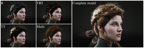
Figure 14.49. Real-time hair rendering with the R, TT, and TRT, as well as a multiple scattering component. (Image courtesy of Epic Games, Inc. [863,1802].)

Each BSDF model presented above is complex, expensive to evaluate, and mostly used in movie production path-tracing environments. Thankfully, real-time versions exist. Scheuermann proposes an ad hoc BSDF model that is easy to implement, fast to render, and looks convincing on hair rendered as large quad ribbons [1560]. Going further, it is possible to use the Marschner model [1128] in real time by storing the BSDF in LUT textures indexed by the in and out directions as parameters [1274]. However, this method can make it hard to render a hair with a spatially varying appearance. To avoid this issue, a recent physically based real-time model [863] approximates components from previous work with simplified mathematics to achieve convincing results. See Figure 14.49. However, there is a gap in quality with all these real-time hair rendering models as compared to offline results. The simplified algorithms usually do not feature advanced volumetric shadowing or multiple scattering. Such effects are particularly important for hair with low absorption, e.g., blond hair.

Figure 14.50. Left: using a depth difference from the first occluder with constant extinction coefficients results in too smooth volumetric shadows. Middle: using deep shadow maps [1953] makes it possible to achieve more transmittance variations matching the way hairs are clumped together within the hair volume. Right: combining deep shadow maps with PCSS achieves smoother volumetric shadows based on the distance to the first occluder (see Section for more details). (Image rendered using a hair model courtesy of USC-HairSalon [781].)

In the case of volumetric shadows, recent solutions [36,863] rely on a transmittance value computed using d as the distance along the light’s direction from the first hair encountered to the current fiber according to a constant absorption $σ_{a}$ . This approach is practical and straightforward since it relies on the usual shadow map available in any engine. However, it cannot represent local density variations resulting from clumped hair strands, which is especially important for brightly lit hair. See Figure 14.50. To address this, a volumetric shadow representation can be used (Section ).

Multiple scattering is an expensive term to evaluate when rendering hair. There are not many solutions suitable for real-time implementation. Karis [863] proposes a way to approximate multiple scattering. This ad hoc model uses fake normals (similar to bent normals), wrapped diffuse lighting, and the hairs’ base color raised to a depth-dependent power before it is multiplied with lighting, approximating color saturation after light has scattered through many strands.

A more advanced dual-scattering technique has been presented by Zinke et al. [1972]. See Figure 14.51. It is dual because it evaluates the amount of scattered light according to two factors. First, a global transmittance factor $Ψ^{G}$ is evaluated by combining the BSDF of each hair strand encountered between the shaded pixel and the light’s position. Thus, $Ψ^{G}$ gives the amount of transmittance to apply to the incoming radiance at the shaded position. This value can be evaluated on the GPU by counting the number of hairs and calculating the mean strand orientation on a light path, the latter influencing the BSDF and so also the transmittance. Accumulating these data can be achieved using deep opacity mapping [1953] or occupancy maps [1646]. Second, a local scattering component $Ψ^{L}$ approximates the fact that the transmitted radiance at the shaded position will scatter in the hair fibers around the current one and contribute to the radiance. Both these terms are added as $Ψ^{G} + Ψ^{G} Ψ^{L}$ and fed through the pixel strand BSDF to accumulate the light source contribution. This technique is more expensive, but it is an accurate real-time approximation to the light multiple scattering phenomenon within hair volumes. It can also be used with any of the BSDFs presented in this chapter.

Figure 14.51. The first two images present hair rendered using path tracing as a reference for the three hair scattering components (R, TT, TRT) in isolation and then with multiple scattering added. The last two images present results using the dual-scattering approximation: path-traced and then rendered in real time on the GPU. (Images courtesy of Arno Zinke and Cem Yuksel [1953].)

Environment lighting is another input that is complex to evaluate for animated translucent materials. It is common to simply sample the irradiance from spherical harmonics. The lighting can also be weighted by non-directional pre-integrated ambient occlusion computed from the hair at its rest position [1560]. Using the same fake normal as for multiple scattering, Karis proposes an ad hoc model for environment lighting [863].

For more information, a comprehensive real-time hair rendering course is available online from Yuksel and Tariq [1954]. Before reading research papers and learning more details, this course will teach you all about the many areas of hair rendering such as simulation, collision, geometry, BSDF, multiple scattering, and volumetric shadows. Hair can look convincing in real-time applications. However, much research is still needed to be able to better approximate physically based environment lighting and multiple scattering in hair.

14.7.3. Fur

As opposed to hair, fur is usually seen as short and semi-organized strands typically found on animals. A concept related to the method of using layers of textures for volumetric rendering is volumetric textures, which are volume descriptions that are represented by layers of two-dimensional, semitransparent textures [1203].

For example, Lengyel et al. [1031] use a set of eight textures to represent fur on a surface. Each texture represents a slice through a set of hairs at a given distance from the surface. The model is rendered eight times, with a vertex shader program moving each triangle slightly outward along its vertex normals each time. In this way, each successive model depicts a different height above the surface. Nested models created this way are called shells. This rendering technique falls apart along object silhouette edges, as the hairs break up into dots as the layers spread out. To hide this artifact, the fur is also represented by a different hair texture applied on fins generated along the silhouette edges. See Figure 14.52

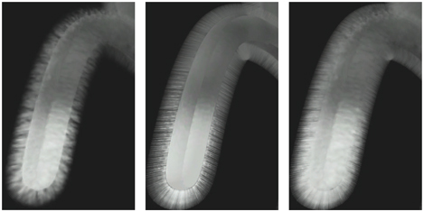
Figure 14.52. Fur using volumetric texturing. The model is rendered eight times, with the surface expanding outward a small amount each pass. On the left is the result of the eight passes. Note the hair breakup along the silhouettes. In the middle, fin rendering is shown. On the right is the final rendering, using both fins and shells. (Images from NVIDIA SDK 10 [1300] sample “Fur—Shells and Fins,” courtesy of NVIDIA Corporation.)

and Figure on page 855. The idea of silhouette fin extrusion can be used to create visual complexity for other types of models. For example, Kharlamov et al. [887] use fins and relief mapping to provide tree meshes with complex silhouettes.

The introduction of the geometry shader made it possible to actually extrude polyline hairs for surfaces with fur. This technique was used in Lost Planet [1428]. A surface is rendered and values are saved at each pixel: fur color, length, and angle. The geometry shader then processes this image, turning each pixel into a semitransparent polyline. By creating one hair per pixel covered, level of detail is automatically maintained. The fur is rendered in two passes. Fur pointing downward in screen space is rendered first, sorted from the bottom to the top of the screen. In this way, blending is performed correctly, back to front. In the second pass, the rest of the fur pointing up is rendered top to bottom, again blending correctly. As the GPU evolves, new techniques become possible and profitable.

It is possible to also use the techniques presented in the previous sections. Strands can be rendered as quads extruded as geometry from a skinned surface such as for Chewbacca in the Star Wars Battlefront games or for the TressFX Rat demo [36]. When rendering hair strands as thin filaments, Ling-Qi et al. [1052] have proven that it is not enough to simulate hair as a uniform cylinder. For animal fur, the medulla is much darker and larger relative to the hair radius. This reduces the impact of light scattering. As such, a double-cylinder fiber BSDF model is presented that simulates a wider range of hair and fur [1052]. It considers more detailed paths such as TttT, TrRrT, TttRttT, and more, where lowercase letters represent interactions with the medulla. This complex approach results in more realistic visuals, especially for simulation of rougher fur and elaborate scattering effects. Such fur rendering techniques involve the rasterization of many strand instances, and anything that can help to reduce the render time is welcome. Ryu [1523] proposes to decimate the number of strand instances rendered as a level of detail scheme dependent on motion magnitude and distance. This method was used for offline movie rendering and appears to be straightforward to apply in real-time applications.

14.8 Unified Approaches

We have reached a point where volumetric rendering has become affordable in real-time applications. What may be possible to achieve in the future?

At the beginning of this chapter we stated that “everything is scattering.” Looking at participating media materials, it is possible to use a high scattering coefficient $σ_{s}$ in order to achieve a opaque medium. This, together with a complex anisotropic phase function driving diffuse and specular responses, would result in an opaque surface material. In light of that, would there be a way to unify solid and volumetric material representations?

As of today, volumetric and opaque material rendering are separated because the current computational capabilities of GPUs force us to use specific approaches that are efficient for some use cases. We use meshes for opaque surfaces, alpha-blended meshes for transparent materials, particle billboards for smoke volumes, and ray marching for some of the volumetric lighting effects within participating media.

As hinted at by Dupuy et al. [397], it may be possible to represent solid and participating media using a unified representation. One possible representation is to use symmetrical GGX [710] (SGGX), an extension of the GGX normal distribution function presented in Section 9.8.1. In this case, the microflake theory representing oriented flake particles within a volume replaces the microfacet theory used for surface normal distribution representation. In a sense, level of detail would become more practical, as compared to meshes, because it can simply become a volume filtering over the material properties. That could lead to more coherent lighting and representation of large detailed worlds while maintaining lighting, shape, occlusion, or transmittance applied over the background. For example, as shown in Figure 14.53, rendering a forest with a volume filtered tree representation would remove visible tree mesh LOD switching, providing a smooth filtering of thin geometry and avoiding aliasing caused by branches, while also providing the correct occlusion value over the background considering the underlying tree geometry within each voxel.

Figure 14.53. A forest rendered using SGGX at the top, with decreasing levels of detail from left to right. The bottom part shows the raw unfiltered voxels. (Images courtesy of Eric Heitz et al. [710].)

Table of Contents for 14 Volumetric and Translucency Rendering

Create new playlist

Sign In

Sign Up