
Chapter 9
Physically Based Shading
“Let the form of an object be what it may,—light, shade, and perspective will always make it beautiful.”
—John Constable
In this chapter we cover the various aspects of physically based shading. We start with a description of the physics of light-matter interaction in Section 9.1, and in Sections 9.2 to 9.4 we show how these physics connect to the shading process. Sections 9.5 to 9.7 are dedicated to the building blocks used to construct physically based shading models, and the models themselves—covering a broad variety of material types—are discussed in Sections 9.8 to 9.12. Finally, in Section 9.13 we describe how materials are blended together, and we cover filtering methods for avoiding aliasing and preserving surface appearance.
9.1 Physics of Light
The interactions of light and matter form the foundation of physically based shading. To understand these interactions, it helps to have a basic understanding of the nature of light.

Figure 9.1. Light, an electromagnetic transverse wave. The electric and magnetic field vectors oscillate at 90∘
In physical optics, light is modeled as an electromagnetic transverse wave, a wave that oscillates the electric and magnetic fields perpendicularly to the direction of its propagation. The oscillations of the two fields are coupled. The magnetic and electric field vectors are perpendicular to each other and the ratio of their lengths is fixed. This ratio is equal to the phase velocity, which we will discuss later.
In Figure 9.1 we see a simple light wave. It is, in fact, the simplest possible—a perfect sine function. This wave has a single wavelength, denoted with the Greek letter λ
The light wave in Figure 9.1 is unusually simple in another respect. It is linearly polarized. This means that for a fixed point in space, the electric and magnetic fields each move back and forth along a line. In contrast, in this book we focus on unpolarized light, which is much more prevalent. In unpolarized light the field oscillations are spread equally over all directions perpendicular to the propagation axis. Despite their simplicity, it is useful to understand the behavior of monochromatic, linearly polarized waves, since any light wave can be factored into a combination of such waves.
If we track a point on the wave with a given phase (for example, an amplitude peak) over time, we will see it move through space at a constant speed, which is the wave’s phase velocity. For a light wave traveling through a vacuum, the phase velocity is c, commonly referred to as the speed of light, about 300,000 kilometers per second.
In Section 8.1.1 we discussed the fact that for visible light, the size of a single wavelength is in the range of approximately 400–700 nanometers. To give some intuition for this length, it is about a half to a third of the width of a single thread of spider silk, which is itself less than a fiftieth of the width of a human hair. See Figure 9.2. In optics it is often useful to talk about the size of features relative to light wavelength. In this case we would say that the width of a spider silk thread is about 2λ

Figure 9.2. On the left visible light wavelengths are shown relative to a single thread of spider silk, which is a bit over 1 micron in width. On the right a similar thread of spider silk is shown next to a human hair, to give some additional context. (Images courtesy of URnano/University of Rochester.)
Light waves carry energy. The density of energy flow is equal to the product of the magnitudes of the electric and magnetic fields, which is—since the magnitudes are proportional to each other—proportional to the squared magnitude of the electric field. We focus on the electric field since it affects matter much more strongly than the magnetic field. In rendering, we are concerned with the average energy flow over time, which is proportional to the squared wave amplitude. This average energy flow density is the irradiance, denoted with the letter E. Irradiance and its relation to other light quantities were discussed in Section 8.1.1.
Light waves combine linearly. The total wave is the sum of the component waves. However, since irradiance is proportional to the square of the amplitudes, this would seem to lead to a paradox. For example, would summing two equal waves not lead to a “ 1+1=4

Figure 9.3. Three scenarios where n monochromatic waves with the same frequency, polarization, and amplitude are added together. From left to right: constructive interference, destructive interference, and incoherent addition. In each case the amplitude and irradiance of the combined wave (bottom) is shown relative to the n original waves (top).
To illustrate, we will look at a simple case: the addition of n monochromatic waves, identical except for phase. The amplitude of each of the n waves is a. As mentioned earlier, the irradiance E1
Figure 9.3 shows three example scenarios for this case. On the left, the waves all line up with the same phase and reinforce each other. The combined wave irradiance is n2
Constructive and destructive interference are two special cases of coherent addition, where the peaks and troughs of the waves line up in some consistent way. Depending on the relative phase relationships, coherent addition of n identical waves can result in a wave with irradiance anywhere between 0 and n2
However, most often when waves are added up they are mutually incoherent, which means that their phases are relatively random. This is illustrated on the right in Figure 9.3. In this scenario, the amplitude of the combined wave is √na

Figure 9.4. Monochromatic waves spreading out from two point sources, with the same frequency. The waves interfere constructively and destructively in different regions of space.
It would seem that destructive and constructive interference violate the conservation of energy. But Figure 9.3 does not show the full picture—it shows the wave interaction at only one location. As waves propagate through space, the phase relationship between them changes from one location to another, as shown in Figure 9.4. In some locations the waves interfere constructively, and the irradiance of the combined wave is greater than the sum of the irradiance values of the individual waves. In other locations they interfere destructively, causing the combined irradiance to be less than the sum of the individual wave irradiance values. This does not violate the law of conservation of energy, since the energy gained via constructive interference and the energy lost via destructive interference always cancel out.
Light waves are emitted when the electric charges in an object oscillate. Part of the energy that caused the oscillations—heat, electrical energy, chemical energy—is converted to light energy, which is radiated away from the object. In rendering, such objects are treated as light sources. We first discussed light sources in Section 5.2, and they will be described from a more physically based standpoint in Chapter .
After light waves have been emitted, they travel through space until they encounter some bit of matter with which to interact. The core phenomenon underlying the majority of light-matter interactions is simple, and quite similar to the emission case discussed above. The oscillating electrical field pushes and pulls at the electrical charges in the matter, causing them to oscillate in turn. The oscillating charges emit new light waves, which redirect some of the energy of the incoming light wave in new directions. This reaction, called scattering, is the basis of a wide variety of optical phenomena.
A scattered light wave has the same frequency as the original wave. When, as is usually the case, the original wave contains multiple frequencies of light, each one interacts with matter separately. Incoming light energy at one frequency does not contribute to emitted light energy at a different frequency, except for specific—and relatively rare—cases such as fluorescence and phosphorescence, which we will not describe in this book.
An isolated molecule scatters light in all directions, with some directional variation in intensity. More light is scattered in directions close to the original axis of propagation, both forward and backward. The molecule’s effectiveness as a scatterer—the chance that a light wave in its vicinity will be scattered at all—varies strongly by wavelength. Short-wavelength light is scattered much more effectively than longer-wavelength light.
In rendering we are concerned with collections of many molecules. Light interactions with such aggregates will not necessarily resemble interactions with isolated molecules. Waves scattered from nearby molecules are often mutually coherent, and thus exhibit interference, since they originate from the same incoming wave. The rest of this section is devoted to several important special cases of light scattering from multiple molecules.
9.1.1. Particles
In an ideal gas, molecules do not affect each other and thus their relative positions are completely random and uncorrelated. Although this is an abstraction, it is a reasonably good model for air at normal atmospheric pressure. In this case, the phase differences between waves scattered from different molecules are random and constantly changing. As a result, the scattered waves are incoherent and their energy adds linearly, as in the right part of Figure 9.3. In other words, the aggregate light energy scattered from n molecules is n times the light scattered from a single molecule.
In contrast, if the molecules are tightly packed into clusters much smaller than a light wavelength, the scattered light waves in each cluster are in phase and interfere constructively. This causes the scattered wave energy to add up quadratically, as illustrated in the left part of Figure 9.3. Thus the intensity of light scattered from a small cluster of n molecules is n2
This process explains why clouds and fog scatter light so strongly. They are both created by condensation, which is the process of water molecules in the air clumping together into increasingly large clusters. This significantly increases light scattering, even though the overall density of water molecules is unchanged. Cloud rendering is discussed in Section 14.4.2.
When discussing light scattering, the term particles is used to refer to both isolated molecules and multi-molecule clusters. Since scattering from multi-molecule particles with diameters smaller than a wavelength is an amplified (via constructive interference) version of scattering from isolated molecules, it exhibits the same directional variation and wavelength dependence. This type of scattering is called Rayleigh scattering in the case of atmospheric particles and Tyndall scattering in the case of particles embedded in solids.
As particle size increases beyond a wavelength, the fact that the scattered waves are no longer in phase over the entire particle changes the characteristics of the scattering. The scattering increasingly favors the forward direction, and the wavelength dependency decreases until light of all visible wavelengths is scattered equally. This type of scattering is called Mie scattering. Rayleigh and Mie scattering are covered in more detail in Section 14.1.
9.1.2. Media
Another important case is light propagating through a homogeneous medium, which is a volume filled with uniformly spaced identical molecules. The molecular spacing does not have to be perfectly regular, as in a crystal. Liquids and non-crystalline solids can be optically homogeneous if their composition is pure (all molecules are the same) and they have no gaps or bubbles.
In a homogeneous medium, the scattered waves are lined up so that they interfere destructively in all directions except for the original direction of propagation. After the original wave is combined with all the waves scattered from individual molecules, the final result is the same as the original wave, except for its phase velocity and (in some cases) amplitude. The final wave does not exhibit any scattering—it has effectively been suppressed by destructive interference.
The ratio of the phase velocities of the original and new waves defines an optical property of the medium called the index of refraction (IOR) or refractive index, denoted by the letter n. Some media are absorptive. They convert part of the light energy to heat, causing the wave amplitude to decrease exponentially with distance. The rate of decrease is defined by the attenuation index, denoted by the Greek letter κ

Figure 9.5. Four small containers of liquid with different absorption properties. From left to right: clean water, water with grenadine, tea, and coffee.
While the phase velocity of light does not directly affect appearance, changes in velocity do, as we will explain later. On the other hand, light absorption has a direct impact on visuals, since it reduces the intensity of light and can (if varying by wavelength) also change its color. Figure 9.5 shows some examples of light absorption.

Figure 9.6. From left to right: water, water with a few drops of milk, water with about 10% milk, whole milk, and opalescent glass. Most of milk’s scattering particles are larger than visible light wavelengths, so its scattering is primarily colorless, with a faint blue tint apparent in the middle image. The scattering particles in the opalescent glass are all smaller than visible light wavelengths and thus scatter blue light more strongly than red light. Due to the split light and dark background, transmitted light is more visible on the left and scattered light is more visible on the right.
Nonhomogeneous media can often be modeled as homogeneous media with embedded scattering particles. The destructive interference that suppresses scattering in homogeneous media is caused by the uniform alignment of molecules, and thus of the scattered waves they produce. Any localized change in the distribution of molecules will break this pattern of destructive interference, allowing scattered light waves to propagate. Such a localized change can be a cluster of a different molecule type, an air gap, a bubble, or density variation. In any case, it will scatter light like the particles discussed earlier, with scattering properties similarly dependent on the cluster’s size. Even gases can be modeled in this way. For these, the “scattering particles” are transient density fluctuations caused by the constant motion of the molecules. This model enables establishing a meaningful value of n for gases, which is useful for understanding their optical properties. Figure 9.6 shows some examples of light scattering.

Figure 9.7. The left image shows that, over a distance of multiple meters, water absorbs light, especially red light, quite strongly. The right image shows noticeable light scattering over multiple miles of air, even in the absence of heavy pollution or fog.
Scattering and absorption are both scale-dependent. A medium that does not produce any apparent scattering in a small scene may have quite noticeable scattering at larger scales. For example, light scattering in air and absorption in water are not visible when observing a glass of water in a room. However, in extended environments both effects can be significant, as shown in Figure 9.7.
In the general case, a medium’s appearance is caused by some combination of scattering and absorption, as shown in Figure 9.8. The degree of scattering determines cloudiness, with high scattering creating an opaque appearance. With somewhat rare exceptions, such as the opalescent glass in Figure 9.6, particles in solid and liquid media tend to be larger than a light wavelength, and tend to scatter light of all visible wavelengths equally. Thus any color tint is usually caused by the wavelength dependence of the absorption. The lightness of the medium is a result of both phenomena. A white color in particular is the result of a combination of high scattering and low absorption. This is discussed in more detail in Section 14.1.

Figure 9.8. Containers of liquids that exhibit varying combinations of absorption and scattering.
9.1.3. Surfaces
From an optical perspective, an object surface is a two-dimensional interface separating volumes with different index of refraction values. In typical rendering situations, the outer volume contains air, with a refractive index of about 1.003, often assumed to be 1 for simplicity. The refractive index of the inner volume depends on the substance from which the object is made.
When a light wave strikes a surface, two aspects of that surface have important effects on the result: the substances on either side, and the surface geometry. We will start by focusing on the substance aspect, assuming the simplest-possible surface geometry, a perfectly flat plane. We denote the index of refraction on the “outside” (the side where the incoming, or incident, wave originates) as n1
We have seen in the previous section that light waves scatter when they encounter a discontinuity in material composition or density, i.e., in the index of refraction. A planar surface separating different indices of refraction is a special type of discontinuity that scatters light in a specific way. The boundary conditions require that the electrical field component parallel to the surface is continuous. In other words, the projection of the electric field vector to the surface plane must match on either side of the surface. This has several implications:
- At the surface, any scattered waves must be either in phase, or 180∘
180∘ out of phase, with the incident wave. Thus at the surface, the peaks of the scattered waves must line up either with the peaks or the troughs of the incident wave. This restricts the scattered waves to go in only two possible directions, one continuing forward into the surface and one retreating away from it. The first of these is the transmitted wave, and the second is the reflected wave. - The scattered waves must have the same frequency as the incident wave. We assume a monochromatic wave here, but the principles we discuss can be applied to any general wave by first decomposing it into monochromatic components.
- As a light wave moves from one medium to another, the phase velocity—the speed the wave travels through the medium—changes proportionally to the relative index of refraction (n1/n2)
(n1/n2) . Since the frequency is fixed, the wavelength also changes proportionally to (n1/n2)(n1/n2) .
The final result is shown in Figure 9.9. The reflected and incident wave directions have the same angle θi
(9.1)
sin(θt)=n1n2sin(θi).This equation for refraction is known as Snell’s law. It is used in global refraction effects, which will be discussed further in Section 14.5.2.

Figure 9.9. A light wave striking a planar surface separating indices of refraction n1
Although refraction is often associated with clear materials such as glass and crystal, it happens at the surface of opaque objects as well. When refraction occurs with opaque objects, the light undergoes scattering and absorption in the object’s interior. Light interacts with the object’s medium, just as with the various cups of liquid in Figure 9.8. In the case of metals, the interior contains many free electrons (electrons not bound to molecules) that “soak up” the refracted light energy and redirect it into the reflected wave. This is why metals have high absorption as well as high reflectivity.
The surface refraction phenomena we have discussed—reflection and refraction—require an abrupt change in index of refraction, occurring over a distance of less than a single wavelength. A more gradual change in index of refraction does not split the light, but instead causes its path to curve, in a continuous analog of the discontinuous bend that occurs in refraction. This effect commonly can be seen when air density varies due to temperature, such as mirages and heat distortion. See Figure 9.10.

Figure 9.10. An example of light paths bending due to gradual changes in index of refraction, in this case caused by temperature variations. (“EE Lightnings heat haze,” Paul Lucas, used under the CC BY 2.0 license.)
Even an object with a well-defined boundary will have no visible surface if it is immersed in a substance with the same index of refraction. In the absence of an index of refraction change, reflection and refraction cannot occur. An example of this is seen in Figure 9.11.

Figure 9.11. The refractive index of these decorative beads is the same as water. Above the water, they have a visible surface due to the difference between their refractive index and that of air. Below the water, the refractive index is the same on both sides of the bead surfaces, so the surfaces are invisible. The beads themselves are visible only due to their colored absorption.
Until now we have focused on the effect of the substances on either side of a surface. We will now discuss the other important factor affecting surface appearance: geometry. Strictly speaking, a perfectly flat planar surface is impossible. Every surface has irregularities of some kind, even if only the individual atoms comprising the surface. However, surface irregularities much smaller than a wavelength have no effect on light, and surface irregularities much larger than a wavelength effectively tilt the surface without affecting its local flatness. Only irregularities with a size in the range of 1–100 wavelengths cause the surface to behave differently than a flat plane, via a phenomenon called diffraction that will be discussed further in Section 9.11.
In rendering, we typically use geometrical optics, which ignores wave effects such as interference and diffraction. This is equivalent to assuming that all surface irregularities are either smaller than a light wavelength or much larger. In geometrical optics light is modeled as rays instead of waves. At the point a light ray intersects with a surface, the surface is treated locally as a flat plane. The diagram on the bottom right of Figure 9.9 can be seen as a geometrical optics picture of reflection and refraction, in contrast with the wave picture presented in the other parts of that figure. We will keep to the realm of geometrical optics from this point until Section 9.11, which is dedicated to the topic of shading models based on wave optics.
As we mentioned earlier, surface irregularities much larger than a wavelength change the local orientation of the surface. When these irregularities are too small to be individually rendered—in other words, smaller than a pixel—we refer to them as microgeometry. The directions of reflection and refraction depend on the surface normal. The effect of the microgeometry is to change that normal at different points on the surface, thus changing the reflected and refracted light directions.

Figure 9.12. On the left we see photographs of two surfaces, with diagrams of their microscopic structures on the right. The top surface has slightly rough microgeometry. Incoming light rays hit surface points that are angled somewhat differently and reflect in a narrow cone of directions. The visible effect is a slight blurring of the reflection. The bottom surface has rougher microgeometry. Surface points hit by incoming light rays are angled in significantly different directions and the reflected light spreads out in a wide cone, causing blurrier reflections.
Even though each specific point on the surface reflects light in only a single direction, each pixel covers many surface points that reflect light in various directions. The appearance is driven by the aggregate result of all the different reflection directions. Figure 9.12 shows an example of two surfaces that have similar shapes on the macroscopic scale but significantly different microgeometry.

Figure 9.13. When viewed macroscopically, surfaces can be treated as reflecting and refracting light in multiple directions.
For rendering, rather than modeling the microgeometry explicitly, we treat it statistically and view the surface as having a random distribution of microstructure normals. As a result, we model the surface as reflecting (and refracting) light in a continuous spread of directions. The width of this spread, and thus the blurriness of reflected and refracted detail, depends on the statistical variance of the microgeometry normal vectors—in other words, the surface microscale roughness. See Figure 9.13.
9.1.4. Subsurface Scattering
Refracted light continues to interact with the interior volume of the object. As mentioned earlier, metals reflect most incident light and quickly absorb the rest. In contrast, non-metals exhibit a wide variety of scattering and absorption behaviors, which are similar to those seen in the cups of liquid in Figure 9.8. Materials with low scattering and absorption are transparent, transmitting any refracted light through the entire object. Simple methods for rendering such materials without refraction were discussed in Section 5.5, and refraction will be covered in detail in Section 14.5.2. In this chapter we will focus on opaque objects, in which the transmitted light undergoes multiple scattering and absorption events until finally some of it is re-emitted back from the surface. See Figure 9.14.

Figure 9.14. The refracted light undergoes absorption as it travels through the material. In this example most of the absorption is at longer wavelengths, leaving primarily short-wavelength blue light. In addition, it scatters from particles inside the material. Eventually some refracted light is scattered back out of the surface, as shown by the blue arrows exiting the surface in various directions.
This subsurface-scattered light exits the surface at varying distances from the entry point. The distribution of entry-exit distances depends on the density and properties of the scattering particles in the material. The relationship between these distances and the shading scale (the size of a pixel, or the distance between shading samples) is important. If the entry-exit distances are small compared to the shading scale, they can be assumed to be effectively zero for shading purposes. This allows subsurface scattering to be combined with surface reflection into a local shading model, with outgoing light at a point depending only on incoming light at the same point. However, since subsurface-scattered light has a significantly different appearance than surface-reflected light, it is convenient to divide them into separate shading terms. The specular term models surface reflection, and the diffuse term models local subsurface scattering.
If the entry-exit distances are large compared to the shading scale, then specialized rendering techniques are needed to capture the visual effect of light entering the surface at one point and leaving it from another. These global subsurface scattering techniques are covered in detail in Section 14.6. The difference between local and global subsurface scattering is illustrated in Figure 9.15.

Figure 9.15. On the left, we are rendering a material with subsurface scattering. Two different sampling sizes are shown, in yellow and purple. The large yellow circle represents a single shading sample covering an area larger than the subsurface scattering distances. Thus, those distances can be ignored, enabling subsurface scattering to be treated as the diffuse term in a local shading model, as shown in the separate figure on the right. If we move closer to this surface, the shading sample area becomes smaller, as shown by the small purple circle. The subsurface scattering distances are now large compared to the area covered by a shading sample. Global techniques are needed to produce a realistic image from these samples.
It is important to note that local and global subsurface scattering techniques model exactly the same physical phenomena. The best choice for each situation depends not only on the material properties but also on the scale of observation. For example, when rendering a scene of a child playing with a plastic toy, it is likely that global techniques would be needed for an accurate rendering of the child’s skin, and that a local diffuse shading model would suffice for the toy. This is because the scattering distances in skin are quite a bit larger than in plastic. However, if the camera is far enough away, the skin scattering distances would be smaller than a pixel and local shading models would be accurate for both the child and the toy. Conversely, in an extreme close-up shot, the plastic would exhibit noticeable non-local subsurface scattering and global techniques would be needed to render the toy accurately.
9.2 The Camera
As mentioned in Section 8.1.1, in rendering we compute the radiance from the shaded surface point to the camera position. This simulates a simplified model of an imaging system such as a film camera, digital camera, or human eye.
Such systems contain a sensor surface composed of many discrete small sensors. Examples include rods and cones in the eye, photodiodes in a digital camera, or dye particles in film. Each of these sensors detects the irradiance value over its surface and produces a color signal. Irradiance sensors themselves cannot produce an image, since they average light rays from all incoming directions. For this reason, a full imaging system includes a light-proof enclosure with a single small aperture (opening) that restricts the directions from which light can enter and strike the sensors. A lens placed at the aperture focuses the light so that each sensor receives light from only a small set of incoming directions. The enclosure, aperture, and lens have the combined effect of causing the sensors to be directionally specific. They average light over a small area and a small set of incoming directions. Rather than measuring average irradiance—which as we have seen in Section 8.1.1 quantifies the surface density of light flow from all directions—these sensors measure average radiance, which quantifies the brightness and color of a single ray of light.
Historically, rendering has simulated an especially simple imaging sensor called a pinhole camera, shown in the top part of Figure 9.16. A pinhole camera has an extremely small aperture—in the ideal case, a zero-size mathematical point—and no lens. The point aperture restricts each point on the sensor surface to collect a single ray of light, with a discrete sensor collecting a narrow cone of light rays with its base covering the sensor surface and its apex at the aperture. Rendering systems model pinhole cameras in a slightly different (but equivalent) way, shown in the middle part of Figure 9.16. The location of the pinhole aperture is represented by the point c
When rendering, each shading sample corresponds to a single ray and thus to a sample point on the sensor surface. The process of antialiasing (Section ) can be interpreted as reconstructing the signal collected over each discrete sensor surface. However, since rendering is not bound by the limitations of physical sensors, we can treat the process more generally, as the reconstruction of a continuous image signal from discrete samples.
Although actual pinhole cameras have been constructed, they are poor models for most cameras used in practice, as well as for the human eye. A model of an imaging system using a lens is shown in the bottom part of Figure 9.16. Including a lens allows for the use of a larger aperture, which greatly increases the amount of light collected by the imaging system. However, it also causes the camera to have a limited depth of field (Section ), blurring objects that are too near or too far.
The lens has an additional effect aside from limiting the depth of field. Each sensor location receives a cone of light rays, even for points that are in perfect focus. The idealized model where each shading sample represents a single viewing ray can sometimes introduce mathematical singularities, numerical instabilities, or visual aliasing. Keeping the physical model in mind when we render images can help us identify and resolve such issues.

Figure 9.16. Each of these camera model figures contains an array of pixel sensors. The solid lines bound the set of light rays collected from the scene by three of these sensors. The inset images in each figure show the light rays collected by a single point sample on a pixel sensor. The top figure shows a pinhole camera, the middle figure shows a typical rendering system model of the same pinhole camera with the camera point c
9.3 The BRDF
Ultimately, physically based rendering comes down to computing the radiance entering the camera along some set of view rays. Using the notation for incoming radiance introduced in Section 8.1.1, for a given view ray the quantity we need to compute is Li(c,-v)
In rendering, scenes are typically modeled as collections of objects with media in between them (the word “media” actually comes from the Latin word for “in the middle” or “in between”). Often the medium in question is a moderate amount of relatively clean air, which does not noticeably affect the ray’s radiance and can thus be ignored for rendering purposes. Sometimes the ray may travel through a medium that does affect its radiance appreciably via absorption or scattering. Such media are called participating media since they participate in the light’s transport through the scene. Participating media will be covered in detail in Chapter 14. In this chapter we assume that there are no participating media present, so the radiance entering the camera is equal to the radiance leaving the closest object surface in the direction of the camera:
(9.2)
Li(c,-v)=Lo(p,v),where p
Following Equation 9.2, our new goal is to calculate Lo(p,v)
In its original derivation [1277] the BRDF was defined for uniform surfaces. That is, the BRDF was assumed to be the same over the surface. However, objects in the real world (and in rendered scenes) rarely have uniform material properties over their surface. Even an object that is composed of a single material, e.g., a statue made of silver, will have scratches, tarnished spots, stains, and other variations that cause its visual properties to change from one surface point to the next. Technically, a function that captures BRDF variation based on spatial location is called a spatially varying BRDF (SVBRDF) or spatial BRDF (SBRDF). However, this case is so prevalent in practice that the shorter term BRDF is often used and implicitly assumed to depend on surface location.
The incoming and outgoing directions each have two degrees of freedom. A frequently used parameterization involves two angles: elevation θ

Figure 9.17. The BRDF. Azimuth angles ϕi
Since we ignore phenomena such as fluorescence and phosphorescence, we can assume that incoming light of a given wavelength is reflected at the same wavelength. The amount of light reflected can vary based on the wavelength, which can be modeled in one of two ways. Either the wavelength is treated as an additional input variable to the BRDF, or the BRDF is treated as returning a spectrally distributed value. While the first approach is sometimes used in offline rendering [660], in real-time rendering the second approach is always used. Since real-time renderers represent spectral distributions as RGB triples, this simply means that the BRDF returns an RGB value.
To compute Lo(p,v)
(9.3)
Lo(p,v)=∫l∈Ωf(l,v)Li(p,l)(n·l)dl.The l∈Ω
In summary, the reflectance equation shows that outgoing radiance equals the integral (over l
For brevity, for the rest of the chapter we will omit the surface point p
(9.4)
Lo(v)=∫l∈Ωf(l,v)Li(l)(n·l)dl. When computing the reflectance equation, the hemisphere is often parameterized using spherical coordinates ϕ
(9.5)
Lo(θo,ϕo)=∫2πϕi=0∫π/2θi=0f(θi,ϕi,θo,ϕo)L(θi,ϕi)cosθisinθidθidϕi.The angles θi
In some cases it is convenient to use a slightly different parameterization, with the cosines of the elevation angles μi=cosθi
(9.6)
Lo(μo,ϕo)=∫2πϕi=0∫1μi=0f(μi,ϕi,μo,ϕo)L(μi,ϕi)μidμidϕi.The BRDF is defined only in cases where both the light and view directions are above the surface. The case where the light direction is under the surface can be avoided by either multiplying the BRDF by zero or not evaluating the BRDF for such directions in the first place. But what about view directions under the surface, in other words where the dot product n·v
The laws of physics impose two constraints on any BRDF. The first constraint is Helmholtz reciprocity, which means that the input and output angles can be switched and the function value will be the same:
(9.7)
f(l,v)=f(v,l).In practice, BRDFs used in rendering often violate Helmholtz reciprocity without noticeable artifacts, except for offline rendering algorithms that specifically require reciprocity, such as bidirectional path tracing. However, it is a useful tool to use when determining if a BRDF is physically plausible.
The second constraint is conservation of energy—the outgoing energy cannot be greater than the incoming energy (not counting glowing surfaces that emit light, which are handled as a special case). Offline rendering algorithms such as path tracing require energy conservation to ensure convergence. For real-time rendering, exact energy conservation is not necessary, but approximate energy conservation is important. A surface rendered with a BRDF that significantly violates energy conservation would be too bright, and so may look unrealistic.
The directional-hemispherical reflectance R(l)
(9.8)
R(l)=∫v∈Ωf(l,v)(n·v)dv.Note that here v
A similar but in some sense opposite function, hemispherical-directional reflectance R(v)
(9.9)
R(v)=∫l∈Ωf(l,v)(n·l)dl.If the BRDF is reciprocal, then the hemispherical-directional reflectance and the directional-hemispherical reflectance are equal and the same function can be used to compute either one. Directional albedo can be used as a blanket term for both reflectances in cases where they are used interchangeably.
The value of the directional-hemispherical reflectance R(l)
The simplest possible BRDF is Lambertian, which corresponds to the Lambertian shading model briefly discussed in Section 5.2. The Lambertian BRDF has a constant value. The well-known (n·l)
(9.10)
R(l)=πf(l,v).The constant reflectance value of a Lambertian BRDF is typically referred to as the diffuse color cdiff
(9.11)
f(l,v)=ρssπ.The 1/π

Figure 9.18. Example BRDFs. The solid green line coming from the right of each figure is the incoming light direction, and the dashed green and white line is the ideal reflection direction. In the top row, the left figure shows a Lambertian BRDF (a simple hemisphere). The middle figure shows Blinn-Phong highlighting added to the Lambertian term. The right figure shows the Cook-Torrance BRDF [285,1779]. Note how the specular highlight is not strongest in the reflection direction. In the bottom row, the left figure shows a close-up of Ward’s anisotropic model. In this case, the effect is to tilt the specular lobe. The middle figure shows the Hapke/Lommel-Seeliger “lunar surface” BRDF [664], which has strong retroreflection. The right figure shows Lommel-Seeliger scattering, in which dusty surfaces scatter light toward grazing angles. (Images courtesy of Szymon Rusinkiewicz, from his “bv” BRDF browser.)
One way to understand a BRDF is to visualize it with the input direction held constant. See Figure 9.18. For a given direction of incoming light, the BRDF’s values are displayed for all outgoing directions. The spherical part around the point of intersection is the diffuse component, since outgoing radiance has an equal chance of reflecting in any direction. The ellipsoidal piece is the specular lobe. Naturally, such lobes are in the reflection direction from the incoming light, with the thickness of the lobe corresponding to the fuzziness of the reflection. By the principle of reciprocity, these same visualizations can also be thought of as how much each different incoming light direction contributes to a single outgoing direction.
9.4 Illumination
The Li(l)
In realistic scenes, Li(l)
Although punctual and directional lights are non-physical abstractions, they can be derived as approximations of physical light sources. Such a derivation is important, because it enables us to incorporate these lights in a physically based rendering framework with confidence that we understand the error involved.
We take a small, distant area light and define lc
With these definitions, a directional light can be derived as the limit case of shrinking the size of the area light down to zero while maintaining the value of clight
(9.12)
Lo(v)=πf(lc,v)clight(n·lc).The dot product (n·l)
(9.13)
Lo(v)=πf(lc,v)clight(n·lc)+. Note the x+
Punctual lights can be treated similarly. The only differences are that the area light is not required to be distant, and clight
(9.14)
Lo(v)=π∑ni=1f(lci,v)clighti(n·lci)+,where lci
The π
9.5 Fresnel Reflectance
In Section 9.1 we discussed light-matter interaction from a high level. In Section 9.3, we covered the basic machinery for expressing these interactions mathematically: the BRDF and the reflectance equation. Now we are ready to start drilling down to specific phenomena, quantifying them so they can be used in shading models. We will start with reflection from a flat surface, first discussed in Section 9.1.3.
An object’s surface is an interface between the surrounding medium (typically air) and the object’s substance. The interaction of light with a planar interface between two substances follows the Fresnel equations developed by Augustin-Jean Fresnel (1788–1827) (pronounced freh-nel). The Fresnel equations require a flat interface following the assumptions of geometrical optics. In other words, the surface is assumed to not have any irregularities between 1 light wavelength and 100 wavelengths in size. Irregularities smaller than this range have no effect on the light, and larger irregularities effectively tilt the surface but do not affect its local flatness.
Light incident on a flat surface splits into a reflected part and a refracted part. The direction of the reflected light (indicated by the vector ri
(9.15)
ri=2(n·l)n-l.See Figure 9.19.

Figure 9.19. Reflection at a planar surface. The light vector l
The amount of light reflected (as a fraction of incoming light) is described by the Fresnel reflectance F, which depends on the incoming angle θi
As discussed in Section 9.1.3, reflection and refraction are affected by the refractive index of the two substances on either side of the plane. We will continue to use the notation from that discussion. The value n1
The Fresnel equations describe the dependence of F on θi
9.5.1. External Reflection
External reflection is the case where n1<n2
For a given substance, the Fresnel equations can be interpreted as defining a reflectance function F(θi)
- When θi=0∘
θi=0∘ , with the light perpendicular to the surface ( l=nl=n ), F(θi)F(θi) has a value that is a property of the substance. This value, F0F0 , can be thought of as the characteristic specular color of the substance. The case when θi=0∘θi=0∘ is called normal incidence. - As θi
θi increases and the light strikes the surface at increasingly glancing angles, the value of F(θi)F(θi) will tend to increase, reaching a value of 1 for all frequencies (white) at θi=90∘θi=90∘ .
Figure 9.20 shows the F(θi)

Figure 9.20. Fresnel reflectance F for external reflection from three substances: glass, copper, and aluminum (from left to right). The top row has three-dimensional plots of F as a function of wavelength and incidence angle. The second row shows the spectral value of F for each incidence angle converted to RGB and plotted as separate curves for each color channel. The curves for glass coincide, as its Fresnel reflectance is colorless. In the third row, the R, G, and B curves are plotted against the sine of the incidence angle, to account for the foreshortening shown in Figure 9.21. The same x-axis is used for the strips in the bottom row, which show the RGB values as colors.
In the case of mirror reflection, the outgoing or view angle is the same as the incidence angle. This means that surfaces that are at a glancing angle to the incoming light—with values of θi

Figure 9.21. Surfaces tilted away from the eye are foreshortened. This foreshortening is consistent with projecting surface points according to the sine of the angle between v
From this point, we will typically use the notation F(n,l)
The increase in reflectance at glancing angles is often called the Fresnel effect in rendering publications (in other fields, the term has a different meaning relating to transmission of radio waves). You can see the Fresnel effect for yourself with a short experiment. Take a smartphone and sit in front of a bright area, such as a computer monitor. Without turning it on, first hold the phone close to your chest, look down at it, and angle it slightly so that its screen reflects the monitor. There should be a relatively weak reflection of the monitor on the phone screen. This is because the normal-incidence reflectance of glass is quite low. Now raise the smartphone up so that it is roughly between your eyes and the monitor, and again angle its screen to reflect the monitor. Now the reflection of the monitor on the phone screen should be almost as bright as the monitor itself.
Besides their complexity, the Fresnel equations have other properties that makes their direct use in rendering difficult. They require refractive index values sampled over the visible spectrum, and these values may be complex numbers. The curves in Figure 9.20 suggest a simpler approach based on the characteristic specular color F0
(9.16)
F(n,l)≈F0+(1-F0)(1-(n·l)+)5.This function is an RGB interpolation between white and F0

Figure 9.22. Schlick’s approximation to Fresnel reflectance compared to the correct values for external reflection from six substances. The top three substances are the same as in Figure 9.20: glass, copper, and aluminum (from left to right). The bottom three substances are chromium, iron, and zinc. Each substance has an RGB curve plot with solid lines showing the full Fresnel equations and dotted lines showing Schlick’s approximation. The upper color bar under each curve plot shows the result of the full Fresnel equations, and the lower color bar shows the result of Schlick’s approximation.
Figure 9.22 contains several substances that diverge from the Schlick curves, exhibiting noticeable “dips” just before going to white. In fact, the substances in the bottom row were chosen because they diverge from the Schlick approximation to an especially large extent. Even for these substances the resulting errors are quite subtle, as shown by the color bars at the bottom of each plot in the figure. In the rare cases where it is important to precisely capture the behavior of such materials, an alternative approximation given by Gulbrandsen [623] can be used. This approximation can achieve a close match to the full Fresnel equations for metals, though it is more computationally expensive than Schlick’s. A simpler option is to modify Schlick’s approximation to allow for raising the final term to powers other than 5 (as in Equation 9.18). This would change the “sharpness” of the transition to white at 90∘
When using the Schlick approximation, F0
(9.17)
F0=(n-1n+1)2.This equation works even with complex-valued refractive indices (such as those of metals) if the magnitude of the (complex) result is used. In cases where the refractive index varies significantly over the visible spectrum, computing an accurate RGB value for F0
In some applications [732,947] a more general form of the Schlick approximation is used:
(9.18)
F(n,l)≈F0+(F90-F0)(1-(n·l)+)1p.This provides control over the color to which the Fresnel curve transitions at 90∘
9.5.2. Typical Fresnel Reflectance Values
Substances are divided into three main groups with respect to their optical properties. There are dielectrics, which are insulators; metals, which are conductors; and semiconductors, which have properties somewhere in between dielectrics and metals.
Fresnel Reflectance Values for Dielectrics
Most materials encountered in daily life are dielectrics—glass, skin, wood, hair, leather, plastic, stone, and concrete, to name a few. Water is also a dielectric. This last may be surprising, since in daily life water is known to conduct electricity, but this conductivity is due to various impurities. Dielectrics have fairly low values for F0
Table 9.1. Values of F0

The F0
Once the light is transmitted into the dielectric, it may be further scattered or absorbed. Models for this process are discussed in more detail in Section 9.9. If the material is transparent, the light will continue until it hits an object surface “from the inside,” which is detailed in Section 9.5.3.
Fresnel Reflectance Values for Metals
Metals have high values of F0
Similarly to Table 9.1, Table 9.2 has linear values as well as 8-bit sRGB-encoded values for texturing. However, here we give RGB values since many metals have colored Fresnel reflectance. These RGB values are defined using the sRGB (and Rec. 709) primaries and white point. Gold has a somewhat unusual F0
Table 9.2. Values of F0

Recall that metals immediately absorb any transmitted light, so they do not exhibit any subsurface scattering or transparency. All the visible color of a metal comes from F0
Fresnel Reflectance Values for Semiconductors
Table 9.3. The value of F0

As one would expect, semiconductors have F0
Fresnel Reflectance Values in Water
In our discussion of external reflectance, we have assumed that the rendered surface is surrounded by air. If not, the reflectance will change, since it depends on the ratio between the refractive indices on both sides of the interface. If we can no longer assume that n1=1
(9.19)
F0=(n1-n2n1+n2)2.Likely the most frequently encountered case where n1≠1
Table 9.4. A comparison between values of F0

Parameterizing Fresnel Values
An often-used parameterization combines the specular color F0
The “metalness” parameter first appeared as part of an early shading model used at Brown University [1713], and the parameterization in its current form was first used by Pixar for the film Wall-E [1669]. For the Disney principled shading model, used in Disney animation films from Wreck-It Ralph onward, Burley added an additional scalar “specular” parameter to control dielectric F0
For those rendering applications that use this metalness parameterization instead of using F0
Using metalness has some drawbacks. It cannot express some types of materials, such as coated dielectrics with tinted F0
Another parameterization trick used by some real-time applications takes advantage of the fact that no materials have values of F0
9.5.3. Internal Reflection
Although external reflection is more frequently encountered in rendering, internal reflection is sometimes important as well. Internal reflection happens when n1>n2

Figure 9.23. Internal reflection at a planar surface, where n1>n2
Snell’s law indicates that, for internal reflection, sinθt>sinθi
The Fresnel equations are symmetrical, in the sense that the incoming and transmission vectors can be switched and the reflectance remains the same. In combination with Snell’s law, this symmetry implies that the F(θi)

Figure 9.24. Comparison of internal and external reflectance curves at a glass-air interface. The internal reflectance curve goes to 1.0 at the critical angle θc
Internal reflection occurs only in dielectrics, as metals and semiconductors quickly absorb any light propagating inside them [285,286]. Since dielectrics have real-valued refractive indices, computation of the critical angle from the refractive indices or from F0
(9.20)
sinθc=n2n1=1-√F01+√F0.The Schlick approximation shown in Equation 9.16 is correct for external reflection. It can be used for internal reflection by substituting the transmission angle θt
9.6 Microgeometry
As we discussed earlier in Section 9.1.3, surface irregularities much smaller than a pixel cannot feasibly be modeled explicitly, so the BRDF instead models their aggregate effect statistically. For now we keep to the domain of geometrical optics, which assumes that these irregularities either are smaller than a light wavelength (and so have no effect on the light’s behavior) or are much larger. The effects of irregularities that are in the “wave optics domain” (around 1–100 wavelengths in size) will be discussed in Section 9.11.
Each visible surface point contains many microsurface normals that bounce the reflected light in different directions. Since the orientations of individual microfacets are somewhat random, it makes sense to model them as a statistical distribution. For most surfaces, the distribution of microgeometry surface normals is continuous, with a strong peak at the macroscopic surface normal. The “tightness” of this distribution is determined by the surface roughness. The rougher the surface, the more “spread out” the microgeometry normals will be.

Figure 9.25. Gradual transition from visible detail to microscale. The sequence of images goes top row left to right, then bottom row left to right. The surface shape and lighting are constant. Only the scale of the surface detail changes.
The visible effect of increasing microscale roughness is greater blurring of reflected environmental detail. In the case of small, bright light sources, this blurring results in broader and dimmer specular highlights. Those from rougher surfaces are dimmer because the light energy is spread into a wider cone of directions. This phenomenon can be seen in the photographs in Figure 9.12 on page 305.
Figure 9.25 shows how visible reflectance results from the aggregate reflections of the individual microscale surface details. The series of images shows a curved surface lit by a single light, with bumps that steadily decrease in scale until in the last image the bumps are much smaller than a single pixel. Statistical patterns in the many small highlights eventually become details in the shape of the resulting aggregate highlight. For example, the relative sparsity of individual bump highlights in the periphery becomes the relative darkness of the aggregate highlight away from its center.
For most surfaces, the distribution of the microscale surface normals is isotropic, meaning it is rotationally symmetrical, lacking any inherent directionality. Other surfaces have microscale structure that is anisotropic. Such surfaces have anisotropic surface normal distributions, leading to directional blurring of reflections and highlights. See Figure 9.26.
Some surfaces have highly structured microgeometry, resulting in a variety of microscale normal distributions and surface appearances. Fabrics are a commonly encountered example—the unique appearance of velvet and satin is due to the structure of their microgeometry [78]. Fabric models will be discussed in Section 9.10.

Figure 9.26. On the left, an anisotropic surface (brushed metal). Note the directional blurring of reflections. On the right, a photomicrograph showing a similar surface. Note the directionality of the detail. (Photomicrograph courtesy of the Program of Computer Graphics, Cornell University.)
Although multiple surface normals are the primary effect of microgeometry on reflectance, other effects can also be important. Shadowing refers to occlusion of the light source by microscale surface detail, as shown on the left side of Figure 9.27. Masking, where some facets hide others from the camera, is shown in the center of the figure.

Figure 9.27. Geometrical effects of microscale structure. On the left, the black dashed arrows indicate an area that is shadowed (occluded from the light) by other microgeometry. In the center, the red dashed arrows indicate an area that is masked (occluded from view) by other microgeometry. On the right, interreflection of light between the microscale structures is shown.
If there is a correlation between the microgeometry height and the surface normal, then shadowing and masking can effectively change the normal distribution. For example, imagine a surface where the raised parts have been smoothed by weathering or other processes, and the lower parts remain rough. At glancing angles, the lower parts of the surface will tend to be shadowed or masked, resulting in an effectively smoother surface. See Figure 9.28.

Figure 9.28. The microgeometry shown has a strong correlation between height and surface normal, where the raised areas are smooth and lower areas are rough. In the top image, the surface is illuminated from an angle close to the macroscopic surface normal. At this angle, the rough pits are accessible to many of the incoming light rays, and so many rays are scattered in different directions. In the bottom image, the surface is illuminated from a glancing angle. Shadowing blocks most of the pits, so few light rays hit them, and most rays are reflected from the smooth parts of the surface. In this case, the apparent roughness depends strongly on the angle of illumination.
For all surface types, the visible size of the surface irregularities decreases as the incoming angle θi
Confirm this for yourself. Roll a sheet of non-shiny paper into a long tube. Instead of looking through the hole, move your eye slightly higher, so you are looking down its length. Point your tube toward a brightly lit window or computer screen. With your view angle nearly parallel to the paper you will see a sharp reflection of the window or screen in the paper. The angle has to be extremely close to 90∘
Light that was occluded by microscale surface detail does not disappear. It is reflected, possibly onto other microgeometry. Light may undergo multiple bounces in this way before it reaches the eye. Such interreflections are shown on the right side of Figure 9.27. Since the light is being attenuated by the Fresnel reflectance at each bounce, interreflections tend to be subtle in dielectrics. In metals, multiple-bounce reflection is the source of any visible diffuse reflection, since metals lack subsurface scattering. Multiple-bounce reflections from colored metals are more deeply colored than the primary reflection, since they are the result of light interacting with the surface multiple times.
So far we have discussed the effects of microgeometry on specular reflectance, i.e., the surface reflectance. In certain cases, microscale surface detail can affect subsurface reflectance as well. If the microgeometry irregularities are larger than the subsurface scattering distances, then shadowing and masking can cause a retroreflection effect, where light is preferentially reflected back toward the incoming direction. This effect occurs because shadowing and masking will occlude lit areas when the viewing and lighting directions differ greatly. See Figure 9.29.

Figure 9.29. Retroreflection due to microscale roughness. Both figures show a rough surface with low Fresnel reflectance and high scattering albedo, so subsurface reflectance is visually important. On the left, the viewing and lighting directions are similar. The parts of the microgeometry that are brightly lit are also the ones that are most visible, leading to a bright appearance. On the right, the viewing and lighting directions differ greatly. In this case, the brightly lit areas are occluded from view and the visible areas are shadowed, leading to a darker appearance.
Retroreflection tends to give rough surfaces a flat appearance. See Figure 9.30.

Figure 9.30. Photographs of two objects exhibiting non-Lambertian, retroreflective behavior due to microscale surface roughness. (Photograph on the right courtesy of Peter-Pike Sloan.)
9.7 Microfacet Theory
Many BRDF models are based on a mathematical analysis of the effects of microgeometry on reflectance called microfacet theory. This tool was first developed by researchers in the optics community [124]. It was introduced to computer graphics in 1977 by Blinn [159] and again in 1981 by Cook and Torrance [285]. The theory is based on the modeling of microgeometry as a collection of microfacets.
Each of these tiny facets is flat, with a single microfacet normal m
An important property of a microfacet model is the statistical distribution of the microfacet normals m
The NDF D(m)

Figure 9.31. Side view of a microsurface. On the left, we see that integrating D(m)(n·m)
In other words, the projection D(m)(n·m)
(9.21)
∫m∈ΘD(m)(n·m)dm=1.The integral is over the entire sphere, represented here by Θ
More generally, the projections of the microsurface and macrosurface onto the plane perpendicular to any view direction v
(9.22)
∫m∈ΘD(m)(v·m)dm=v·n. The dot products in Equations 9.21 and 9.22 are not clamped to 0. The right side of Figure 9.31 shows why. Equations 9.21 and 9.22 impose constraints that the function D(m)
Intuitively, the NDF is like a histogram of the microfacet normals. It has high values in directions where the microfacet normals are more likely to be pointing. Most surfaces have NDFs that show a strong peak at the macroscopic surface normal n
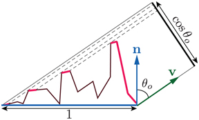
Figure 9.32. Integrating the projected areas of the visible microfacets (in bright red) yields the projected area of the macrosurface onto the plane perpendicular to v
Take a second look at the right side of Figure 9.31. Although there are many microfacets with overlapping projections, ultimately for rendering we care about only the visible microfacets, i.e., the microfacets that are closest to the camera in each overlapping set. This fact suggests an alternative way of relating the projected microfacet areas to the projected macrogeometry area: The sum of the projected areas of the visible microfacets is equal to the projected area of the macrosurface. We can express this mathematically by defining the masking function G1(m,v)
(9.23)
∫∈ΘG1(m,v)D(m)(v·m)+dm=v·n,as shown in Figure 9.32. Unlike Equation 9.22, the dot product in Equation 9.23 is clamped to zero. This operation is shown with the x+
While Equation 9.23 imposes a constraint on G1(m,v)
Although various G1
(9.24)
G1(m,v)=χ+(m·v)1+Λ(v),where χ+(x)
(9.25)
χ+(x)={1,wherex>0,0,wherex≤0.The Λ
The Smith masking function does have some drawbacks. From a theoretical standpoint, its requirements are not consistent with the structure of actual surfaces [708], and may even be physically impossible to realize [657]. From a practical standpoint, while it is quite accurate for random surfaces, its accuracy is expected to decrease for surfaces with a stronger dependency between normal direction and masking, such as the surface shown in Figure 9.28, especially if the surface has some repetitive structure (as do most fabrics). Nevertheless, until a better alternative is found, it is the best option for most rendering applications.
Given a microgeometry description including a micro-BRDF fμ(l,v,m)
(9.26)
f(l,v)=∫m∈Ωfμ(l,v,m)G2(l,v,m)D(m)(m·l)+|n·l|(m·v)+|n·v|dm.This integral is over the hemisphere Ω
Heitz [708] discusses several versions of the G2
(9.27)
G2(l,v,m)=G1(v,m)G1(l,m).This form is equivalent to assuming that masking and shadowing are uncorrelated events. In reality they are not, and the assumption causes over-darkening in BRDFs using this form of G2
As an extreme example, consider the case when the view and light directions are the same. In this case G2
If the microsurface is a heightfield, which is typically the case for microsurface models used in rendering, then whenever the relative azimuth angle ϕ
(9.28)
G2(l,v,m)=λ(ϕ)G1(v,m)G1(l,m)+(1-λ(ϕ))min(G1(v,m),G1(l,m)),where λ(ϕ)
(9.29)
λ(ϕ)=1-e-7.3ϕ2.A different λ
(9.30)
λ(ϕ)=4.41ϕ4.41ϕ+1.Regardless of the relative alignment of the light and view directions, there is another reason that masking and shadowing at a given surface point are correlated. Both are related to the point’s height relative to the rest of the surface. The probability of masking increases for lower points, and so does the probability of shadowing. If the Smith masking function is used, this correlation can be precisely accounted for by the Smith height-correlated masking-shadowing function:
(9.31)
G2(l,v,m)=χ+(m·v)χ+(m·l)1+Λ(v)+Λ(l). Heitz also describes a form of Smith G2
(9.32)
G2(l,v,m)=χ+(m·v)χ+(m·l)1+max(Λ(v),Λ(l))+λ(v,l)min(Λ(v),Λ(l)),where the function λ(v,l)
Out of these alternatives, Heitz [708] recommends the height-correlated form of the Smith function (Equation 9.31) since it has a similar cost to the uncorrelated form and better accuracy. This form is the most widely used in practice [861,947,960], though some practitioners use the separable form (Equation 9.27) [214,1937].
The general microfacet BRDF (Equation 9.26) is not used directly for rendering. It is used to derive a closed-form solution (exact or approximate) given a specific choice of micro-BRDF fμ
9.8 BRDF Models for Surface Reflection
With few exceptions, the specular BRDF terms used in physically based rendering are derived from microfacet theory. In the case of specular surface reflection, each microfacet is a perfectly smooth Fresnel mirror. Recall that such mirrors reflect each incoming ray of light in a single reflected direction. This means that the micro-BRDF fμ(l,v,m)
(9.33)
h=l+v||l+v||.
Figure 9.33. The half vector h
When deriving a specular microfacet model from Equation 9.26, the fact that the Fresnel mirror micro-BRDF fμ(l,v,m)
(9.34)
fspec(l,v)=F(h,l)G2(l,v,h)D(h)4|n·l||n·v|.Details on the derivation can be found in publications by Walter et al. [1833], Heitz [708], and Hammon [657]. Hammon also shows a method to optimize the BRDF implementation by calculating n·h
We use the notation fspec

Figure 9.34. Surface composed of microfacets. Only the red microfacets, which have their surface normal aligned with the half vector h
The use of the half vector in the masking-shadowing function allows for a minor simplification. Since the angles involved can never be greater than 90∘