
Chapter 15: Personalized Medicine, Machine Learning, and Real World Data
15.2 Individualized Treatment Recommendation
15.2.1 The Individualized Treatment Recommendation Framework
15.2.2 Estimating the Optimal Individualized Treatment Rule
15.4 Example Using the Simulated REFLECTIONS Data
15.5 “Most Like Me” Displays: A Graphical Approach
15.5.1 Most Like Me Computations
15.5.2 Background Information: LTD Distributions from the PCI15K Local Control Analysis
15.5.3 Most Like Me Example Using the PCI15K Data Set
15.5.4 Extensions and Interpretations of Most Like Me Displays
Chapters 6–9 in this text demonstrated methods for estimating the causal effect of treatments over a population of interest. In each of these cases, the method estimates the average effect over some population, such as the average effect among the treated or in the full population. Of course, not all patients respond the same to the same medication. The best treatment plan for one patient might not be optimal for a different patient. Targeted therapy has become the norm in drug development in several fields of medicine such as oncology. Treatment guidance for Type II diabetes also acknowledges patient heterogeneity and varying individualized treatment goals (American Diabetes Association 2016). If significant heterogeneity exists in a patient population, in order to optimize patient care it is critical to identify and understand the key driving factors. Ruberg et al. (2010) summarized the challenge well by stating that the goal is to find “the right treatment for the right patient at the right time.” Indeed, physicians and patients are constantly making decisions regarding treatment options based on the available evidence and individualized treatment goals. For instance, in Chapter 8 we used the REFLECTIONS data to estimate the average effect of opioid treatment relative to standard of care on reduction in pain severity over a one-year period as measured by the BPI-Pain scale. However, does the average effect apply for a female patient with insomnia and a recent fibromyalgia diagnosis? Most of the methods in previous chapters address questions about the population, though the local control method of Chapter 7 estimates local (subgroup) effects. Recently, researchers are turning more and more to subgroup identification, predictive algorithms, and machine learning to help address individual treatment questions.
Typically, randomized controlled trials are powered to detect an overall treatment effect and thus are not well designed for personalized medicine research. Given the large sample sizes in many real world data sources, there is great promise for pairing real world data with newer machine learning algorithms for producing evidence supporting personalized medicine. However, use of such data is limited in some disease states by the lack of relevant outcome variables in such data.
Personalized medicine is naturally connected to subgroup identification – the goal is to find factors that drive differential treatment response. Standard regression modeling is one potential solution as significant treatment by covariate interactions in the regression model identifies subgroups of interest (Kehl and Ulm 2006). However, the challenges of subgroup identification in general are well documented (Lagakos 2006, Ruberg et al. 2010). This include multiplicity, lack of pre-specification, and overfitting (lack of predictive ability). Xu et al. (2015) note that misspecification is common as main effect estimation can interfere with covariate-treatment interactions estimation. Lipkovich et al. (2011) proposed directly searching for treatment interactions of interest using a recursive partitioning algorithm rather than attempting to model the full outcome distribution. In fact, there has been an explosion of different methodology approaches to personalized medicine (see Fu and Gopal (2019) for a brief history and overview of methodologies), and some of the methods presented in earlier chapters can be extended for this type of research.
Fu et al. (2016) classified personalized medicine analytic methods into 3 categories: 1) treatment by subgroup interaction detection, 2) Q-Learning (two-step) method, and 3) value function optimization methods. The first class of methods includes regression and classification and regression tree-based methodologies. The second class includes methods that first estimate the treatment effects on an individual basis followed by analyzing the relationships to the “estimated treatment differences” in the second step. Value function optimization approaches define a benefit to be optimized and then find the assignment rules to optimize benefit.
A review of all approaches being used for personalized medicine research would be extensive and is beyond the scope of this chapter. SAS tools such as the GLMSELECT procedure for penalized regression (Gomes 2015) and the machine learning analytics available in SAS Viya (www.sas.com/sas-viya) may prove of great value. Overall, better guidance from simulations across many methods would be valuable to the field. In the sections that follow, we present the individualized treatment recommendation (ITR) framework, which is designed for personalized medicine research. The ITR framework incorporates many of the standard methods and over the last decade has spawned the introduction of several promising methods such as outcome weighted learning for personalized medicine. We focus on this approach both for brevity and because such approaches have demonstrated optimality based on classification theory.
In addition to core analytic solutions, in this chapter we also take a brief look at graphical approaches that are a useful aid for personalized medicine. The “Most Like Me” approach is a straightforward graphical extension of the Local Control methods presented in Chapter 7.
15.2 Individualized Treatment Recommendation
15.2.1 The Individualized Treatment Recommendation Framework
We follow the notation of Fu et al. (2016). For a sample of N patients, i = 1, …, N, the treatment for each patient is denoted by Ti = 1, …., J, Xi represents a set of pre-treatment covariates, Yi the outcome. Let P represent the distribution of (X, T, Y). Let ![]() be a rule that maps a covariate vector X to a recommended treatment from among T = {1, 2, …, J}.
be a rule that maps a covariate vector X to a recommended treatment from among T = {1, 2, …, J}. ![]() is called an individualized treatment rule because it will assign a treatment for each individual patient based on their pre-treatment X-characteristics.
is called an individualized treatment rule because it will assign a treatment for each individual patient based on their pre-treatment X-characteristics.
For any individualized treatment rule ![]() , let Pr be the distribution of (X, T, Y) given that T =
, let Pr be the distribution of (X, T, Y) given that T = ![]() (the treatment assignments follow the ITR rule r(X)). Each rule
(the treatment assignments follow the ITR rule r(X)). Each rule ![]() has an expected outcome across a population of patients denoted by
has an expected outcome across a population of patients denoted by ![]() . This expectation provides the average outcome over the population given that each patient’s treatment was chosen based on the individualized treatment rule
. This expectation provides the average outcome over the population given that each patient’s treatment was chosen based on the individualized treatment rule ![]() and is called the “reward”:
and is called the “reward”:
![]()
This expectation is also referred to as the value function for the individualized treatment rule ![]() Given this notation, the goal is to find the treatment assignment rule r that maximizes
Given this notation, the goal is to find the treatment assignment rule r that maximizes ![]() assuming larger values of Y are better, across all possible assignment rules. The optimal individualized treatment rule (Qian and Murphy (2011), Zhao et al. (2012)) is thus defined as
assuming larger values of Y are better, across all possible assignment rules. The optimal individualized treatment rule (Qian and Murphy (2011), Zhao et al. (2012)) is thus defined as![]() (X) =
(X) = ![]() where argmax represents the values at which the expectation reaches its maximum.
where argmax represents the values at which the expectation reaches its maximum.
Two comments of note here. First, the denominator of the value function involves inverse probability weighting – similar to the causal inference methods of Chapter 8. Thus, these approaches are suitable for RCT and real world data. Second, these methods are not without assumptions. In general, one still needs to assume the causal inference methodology assumptions of Chapter 2: SUTVA, no unmeasured confounding, positivity, and correct modeling.
Lastly, the theoretical support for methods built on this framework is Fisher’s consistency. A classification method is said to be Fisher’s consistent if the recommended treatment from the algorithm has the largest expected reward (best outcome). Methods that have this property are described in the following subsections.
15.2.2 Estimating the Optimal Individualized Treatment Rule
The computational challenge is to find the optimal individualized treatment rule given an observed set of data (![]() , i = 1 to n. A straightforward method for estimating the optimal rule is a two-step (Q-learning) approach which first builds a model to estimate the outcome Y given X and T. Recent common algorithms include penalized regression methods, regression trees and other machine learning algorithms (the HPSPLIT SAS procedure and SAS Viya), and support vector machines. Once a model is fit, the difference between the predicted value under each treatment (choosing the superior outcome between the two predicted values) leads to an individualized treatment rule. However, Zhao et al. (2012) point out that this is not likely to be an optimal rule due to potential overfitting. They proposed an approach directly maximizing the value function.
, i = 1 to n. A straightforward method for estimating the optimal rule is a two-step (Q-learning) approach which first builds a model to estimate the outcome Y given X and T. Recent common algorithms include penalized regression methods, regression trees and other machine learning algorithms (the HPSPLIT SAS procedure and SAS Viya), and support vector machines. Once a model is fit, the difference between the predicted value under each treatment (choosing the superior outcome between the two predicted values) leads to an individualized treatment rule. However, Zhao et al. (2012) point out that this is not likely to be an optimal rule due to potential overfitting. They proposed an approach directly maximizing the value function.
Zhao et al. (2012) showed that maximizing the value function is equivalent to minimizing the weighted classification error
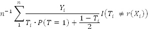
over all possible treatment assignment rules. By replacing the indicator function with a hinge loss function, Zhao transformed the computation into an outcome weighted classification problem and solved the problem using support vector machine methodology. The approach is called outcome weighted learning and has demonstrated superior performance to the two-stage (Q-learning) approaches especially for smaller sample sizes (Chen et al. 2016). In addition, this approach was shown to have Fisher’s consistency.
Fu et al. (2016) used the ITR outcome weighted learning framework but approached the solution from a subgroup identification approach. They used an intuitive comprehensive search algorithm to simplify the computation and interpretation. For two treatment options, the optimal ITR is simply
![]()
The component expectations could be estimated by the familiar inverse weighting formulas,
![]() and
and ![]() Fu et al. (2016) noted some of the benefits of the approach, including the applicability to both RCT and real world data, as well as to continuous, binary, and time to event data.
Fu et al. (2016) noted some of the benefits of the approach, including the applicability to both RCT and real world data, as well as to continuous, binary, and time to event data.
Zheng et al. (2017) extended the outcome weighted learning approach of Zhou et al. (2012) to scenarios with greater than two treatments. That is, scenarios where the patient and physician have more than two treatment options available to choose from. Specifically, they proposed a multi-category outcome weighted learning (MOWL) approach that uses the concept of angle-based classification from Zhang and Liu (2014). Instead of optimizing a single value function, we now construct k-1 functions that map the patient’s covariates into a k-1 dimensional vector. This introduces k angles – one with each potential treatment selection – where the rule then selects the treatment with the smallest angle to the patient’s vector. See Zheng et al. (2017) or Liang et al. (2018) for additional details. Liang et al. (2016) further extended the work to allow for assessing combination of treatments. As with the two-treatment case, the MOWL approach is Fisher’s consistent. The program presented in the following section is based on this multi-category ITR approach.
Program 15.1: Individual Treatment Recommendation
**************************************************************************
* Individual Treatment Recommendation (ITR) *
* Based on: Chong Zhang, et al.: “Multicategory Outcome Weighted Margin- *
* based Learning for Estimating Individualized Treatment Rules”, *
* Statistica Sinica, 2017. *
**************************************************************************;
**************************************************************************
Step 1. Data preparation
a. missing data imputation
b. fitting multinomial PS model
c. trimming
d. converting cohorts into consecutive numbers 1,2,3,...
e. splitting the trimmed data into 3 bins
f. converting class covariates into 0/1 indicators
**************************************************************************;
*** 1a. data preparation and missing data imputation;
Options VALIDVARNAME=V7;
data dat;
set REFL;
run;
* we will use categorized version of DxDur with 99 as missing value;
proc rank data=dat out=tmp groups=3;
var DxDur;
ranks DxDurCat;
run;
data dat;
set tmp;
if DxDurCat=. then DxDurCat=99; else DxDurCat=DxDurCat+1;
chgBPIPain_LOCF=BPIPain_LOCF-BPIPain_B;
if chgBPIPain_LOCF>.; * we have 2 obs with missing Y;
run;
* baseline variables for ITR & PS models;
* categorical variables;
%let pscat=
Gender
Race
DxDurCat
DrSpecialty;
* continuous variables;
%let pscnt=
Age
BMI_B
BPIInterf_B
BPIPain_B
CPFQ_B
FIQ_B
GAD7_B
ISIX_B
PHQ8_B
PhysicalSymp_B
SDS_B;
*** 1b. estimate propensity scores;
* identify Xs associated with outcome;
proc glmselect data=dat namelen=200;
class &pscat;
model chgBPIPain_LOCF=&pscat &pscnt
/selection=stepwise hier=none;
ods output ParameterEstimates=yPE;
run;
proc sql noprint;
select distinct effect into :yeffects separated by ‘ ‘
from yPE
where effect~=’Intercept’
;
select count(distinct effect) into :nyeff
from yPE
where effect~=’Intercept’
;
quit;
* force Xs associated with outcome into PS model;
proc logistic data = dat namelen=200;
class cohort &pscat/param=ref;
model cohort = &yeffects &pscat &pscnt
/link=glogit include=&nyeff selection=stepwise sle=.20 sls=.20 hier=none;
output out=gps pred=ps;
ods output ParameterEstimates=gps_pe;
run;
*** 1c. trimming;
proc transpose data=gps out=gpsdatt prefix=ps;
by subjid cohort;
var ps;
run;
* based on Crump et al. (2009);
%let lambda=;
proc iml;
use gpsdatt(keep=ps:); read all into pscores; close gpsdatt;
start obj1(alpha) global(gx);
uid=gx<alpha;
return(mean(gx#uid)/mean(uid));
finish;
start obj(alpha) global(gx);
uid=gx<alpha;
return(mean(gx#uid)/mean(uid)##2);
finish;
gx=(1/pscores)[,+];
mx0=median(gx);
call nlpnms(rc,xr,’obj’) x0=mx0;
xr=2#obj1(xr);
*one step is often sufficient, i.e. the later integration does not change the
value of alpha. To be safe, you can iterate;
xr=2#obj1(xr);
call symputx(‘lambda’,xr);
create gx var {gx}; append; close gx;
quit;
data gpsdatt;
merge gpsdatt gx;
trim=gx>λ
run;
title1 “trimming details”;
proc freq data=gpsdatt;
table trim*cohort;
run;
title1;
data gps;
merge gps gpsdatt(keep=subjid trim);
by subjid;
if ~trim;
drop trim;
run;
data dpat;
set gps;
if cohort=_level_;
OnOpt_IPW=1/ps;
run;
*** 1d. create numerical equivalent (_leveln_) of the &cohort;
proc sql;
create table cohorts as
select distinct cohort
from dpat
;
quit;
* we will need the format to report this numerical &cohort;
data cohorts;
set cohorts;
cohortn=_n_;
fmtname=’cohort’;
cfmtname=’$cohort’;
run;
proc format cntlin=cohorts(rename=(cohortn=start cohort=label));
run;
proc format cntlin=cohorts(drop=fmtname rename=(cohort=start cohortn=label cfmtname=fmtname));
run;
* add numerical &cohort;
data dpat;
set dpat;
cohortn=input(put(cohort,$cohort.),best.);
run;
*** 1e. inpdat will be split into 3 bins;
data inpdat;
set dpat;
bin=ranuni(117117);
run;
proc rank data=inpdat out=inpdat groups=3;
var bin;
run;
data inpdat;
set inpdat;
bin=bin+1;
label bin=”Bin”;
* Reward: for ITR has to be “the higher the better” so we change the sign of the
original outcome;
Rwrd=-chgBPIPain_LOCF;
Atrt=cohortn; * numerical treatment: for ITR trt. has to be 1,2, ...;
run;
title1 “descriptive statistics”;
proc tabulate data=inpdat;
class cohort bin &pscat;
var &pscnt chgBPIPain_LOCF;
table all (bin &pscat)*(N ColPctN)
(&pscnt chgBPIPain_LOCF)*(NMiss Mean Std Min Max),cohort all;
run;
title1;
*** 1f. convert categorical variables into 0/1 indicators;
proc logistic data=inpdat outdesign=inpdat2 outdesignonly;
class &pscat/param=ref;
model subjid=&pscat &pscnt
/noint;
run;
* final dataset for ITR;
data final;
merge inpdat(keep=subjid cohort &pscat Atrt Rwrd bin chgBPIPain_LOCF) inpdat2;
by subjid;
run;
* store names of baseline Xs into xlst;
proc contents data=inpdat2(drop=subjid) out=inpdat2c;
run;
proc sql;
select name into :xlst separated by ‘ ‘ from inpdat2c where name~=’Intercept’;
quit;
/******************************************************************************
Step 2: ITR linear solver: ITRabcLin_train
This estimates optimal treatment assignment which maximizes the “value function.”
The value function is just the sum(reward*IPW)/nobs where sum is over pts
who have actual treatment the same as the estimated optimal treatment
and nobs is the total number of pts. IPW comes from multinomial PS model.
Reward is the desired outcome (the more positive the better). In our case it is chgBPIPain_LOCF as the desired outcome is to have the decrease in pain.
Detailed Description: the ITR linear solver has 2 hyper-parameters: c (cost) and lambda (penalty)
if c=0 then the classifier is soft and if c=infinity then the classifier is hard.
“Soft classifiers explicitly estimate the class conditional probabilities and then perform classification based on estimated probabilities. In contrast, hard classifiers directly target on the classification decision boundary without producing the probability estimation.” Liu et al. The “optimal” c can be somewhere between 0 and infinity.
lambda penalizes the complexity of the model which predicts the optimal treatment.
The tuning (grid search) on dat finds the c and lambda which maximize the CV value function. Then such values of c and lambda are used to build the ITR model on all data dat.
*****************************************************************************/
/*** macro to train the linear ITR model
The linear solver has 2 hyper-parameters: c (cost) and lambda
The optimal values for c & lambda are found via cross-validated grid search (objective function to maximize the value function);
%macro ITRabcLin_train(
dat=, /*input data set with training data*/
X=, /*list baseline covariates: separated with blanks*/
A=, /*actual treatment variable*/
W=, /*IPW variable: IPW for the actual treatment*/
R=, /*reward (outcome) variable: the higher the better*/
out=ITRabcLin_train_out, /*output dataset with estimated optimal treatment*/
D=est_opt_trt, /*name of estimated optimal treatment variable to be
added on &out*/
betas=ITRabcLin_train_betas, /*output datasets with estimated betas*/
val=ITRabcLin_train_values, /*dataset with CV results and value function*/
nfolds=5, /*number of folds for CV*/
F=foldN, /*name of the folds variable: to be added on &out*/
foldsv=, /*name of the variable with user provided folds for CV: on &dat*/
c_grid=2**do(-10,10,2), /*grid search points for c*/
lambda_grid=2**do(-10,20,1), /*grid search points for lambda*/
tc={20000 50000 . 1e-12}, /*optimization termination criteria: see IML help for
nlpdd*/
opt={. 0}, /*optimization options: see IML help for nlpdd*/
seed=123 /* seed for CV folds */
);
/*** All X, A, W, R, and foldsv variables have to be numerical. I.e. all categorical Xs have to be re-coded into numerical indicator variables;
A should be integer: consecutive numbers starting with 1. So e.g. for 5 arms, it should be coded as 1,2,3,4,5. The same with foldsv (if provided by user).
tc={20000 50000 . 1e-12}
20000 - max. #iterations
50000 - max #obj.function calls
1e-12 - relative function criterion (FTOL)
opt={. 0}
0 - no optimization trace info: if >0 (e.g. 1) then optimization details will be printed;/
%local k; * #trt.arms;
proc sql noprint;
select count(distinct &A) into :k from &dat;
quit;
*** linear solver;
proc iml;
use &dat;
read all var {&X} into x;
read all var {&A} into y;
read all var {&R} into reward;
read all var {&W} into weight;
%if &foldsv> %then read all var {&foldsv} into binN;;
close &dat;
*##############################################################;
start XI_gen(dum) global(k);
XI = J(k-1,k,0);
XI[,1]=repeat((k-1)##(-1/2),k-1,1);
do ii=2 to k;
XI[,ii]=repeat( -(1+sqrt(k))/((k-1)##(1.5)), k-1,1);
XI[ii-1,ii]=XI[ii-1,ii]+sqrt(k/(k-1));
end;
return(XI);
finish;
*##############################################################;
start pred(f);
y=min(loc(f=max(f)));
return(y);
finish;
*##############################################################;
start pred_vertex_MLUM(x_test, t) global(np,k);
XI=XI_gen(.);
beta=J(np,k-1,0);
beta0=repeat(0,1,k-1);
do ii=1 to (k-1);
beta[,ii]=t[ ((np+1)#ii-np) : ((np+1)#ii-1) ];
beta0[ii]=t[ii#(np+1)];
end;
f_matrix = t(t(x_test * beta)+t(beta0));
nr=nrow(x_test);
inner_matrix=J(nr,k, 0);
do ii=1 to k;
inner_matrix[,ii] = (t(t(f_matrix)#XI[,ii]))[,+];
end;
z=j(1,nr,.);
do ii=1 to nr;
z[ii]=pred(inner_matrix[ii,]);
end;
return(z);
finish;
*##############################################################;
start Y_matrix_gen(dum) global(k,nobs,y_train);
Y_matrix = J(nobs,k-1,0);
XI=XI_gen(.);
do ii=1 to nobs;
Y_matrix[ii,] = T(XI[,y_train[ii]]);
end;
return(Y_matrix);
finish;
*##############################################################;
start fir_der(u) global(indicator,c);
z=repeat(-1,1,ncol(u));
if c=.I then do;
index = loc( (u#indicator)=1 );
if ncol(index)>0 then z[index] = .5;
index = loc( (u#indicator)>1 );
if ncol(index)>0 then z[index] = 0;
end; else do;
index = loc( (u#indicator)>=(c/(1+c)) );
if ncol(index)>0 then z[index] = -((1/( (1+c)#(u#indicator)[index]-c+1
))##2);
end;
return(z);
finish;
* loss function;
start orig(u) global(indicator,c);
z=1-u#indicator;
if c=.I then do;
index = loc( (u#indicator)>=1 );
if ncol(index)>0 then z[index] = 0;
end; else do;
index = loc( (u#indicator)>=(c/(1+c)) );
if ncol(index)>0 then z[index]= 1/(1+c) # (1/( (1+c)#(u#indicator)[index]-c+1 ));
end;
return(z);
finish;
*#############################################################;
* return ABM obj function;
start fr_linear(t) global(x_train,y_train,k,c_weight,np,nobs,lambda,Y_matrix);
beta=j(np,k-1,0);
beta0=repeat(0,1,k-1);
do ii=1 to (k-1);
beta[,ii]=t[ ((np+1)#ii-np) : ((np+1)#ii-1) ];
beta0[ii]=t[ii#(np+1)];
end;
f_matrix = t(t(x_train * beta)+t(beta0));
z=sum( c_weight # orig( t((Y_matrix # f_matrix)[,+])) ) / nobs;
z = z+ lambda#sum(beta##2);
return(z);
finish;
*##############################################################;
* return derivative vector of z wrt t;
start grr_linear(t) global(x_train,y_train,k,indicator,c_weight,np,nobs,lambda,Y_matrix);
z=j(1,ncol(t),.);;
beta=j(np,k-1,0);
beta0=repeat(0,1,k-1);
do ii=1 to (k-1);
beta[,ii]=t[ ((np+1)#ii-np) : ((np+1)#ii-1) ];
beta0[ii]=t[ii#(np+1)];
end;
f_matrix = t(t(x_train * beta)+t(beta0));
temp = fir_der( t((Y_matrix # f_matrix)[,+]));
do j=1 to (k-1); *## j= 1 to k-1 for different parts of derivatives;
z[((np+1)#j-np):((np+1)#j-1)] =
(Y_matrix[,j]#t(c_weight#indicator#temp)#x_train)[:,];
z[((np+1)#j-np):((np+1)#j-1)] = z[((np+1)#j-np):((np+1)#j-1)] +
2#lambda*beta[,j];
z[(np+1)#j] = sum( Y_matrix[,j]#t(c_weight#indicator#temp) )/nobs;
end; *# for (j in 1:(k-1)) ## j= 1 to k-1 for different parts of derivatives;
return(z);
finish;
*##############################################################;
* mowl.linear;
start mowl_linear_zk(dum) global (k, np);
betas = repeat(0,1,((k-1)#(np+1)));
call nlpdd(rc,xr,’fr_linear’) x0=betas grd=’grr_linear’ tc=&tc opt=&opt;
betas = xr;
return(betas);
finish;
*##############################################################;
*** main code;
* grid search space for tuning c & lambda;
c_grid=&c_grid;
lambda_grid=&lambda_grid;
k=&k;* #trt.arms;
np = ncol(x); * #baseline Xs;
%if &foldsv= %then %do;
* split into nfolds bins (within trt.arm);
start RandPerm(x); * random permutation of elements of vector x;
u = 1:ncol(x);
call randgen(u, “Uniform”);
return(x[,rank(u)]);
finish;
call randseed(&seed);
bins=RandPerm(1:&nfolds);
binN=j(1,nrow(x),.);
do ik=1 to k;
xbin=RandPerm(loc(y=ik));
do in=&nfolds to 1 by -1;
nbin=max(1,round(ncol(xbin)/in));
binN[,xbin[,1:nbin]]=bins[in];
if in>1 then xbin=xbin[,(nbin+1):ncol(xbin)];
end;
end;
%end; %else %do;
* folds are provided by user;
binN=t(binN);
%end;
* tuning of c & lambda via CV;
valMax=.;
c_best=.;
lambda_best=.;
vals_best=.;
do ic=1 to ncol(c_grid);
c=c_grid[ic];
do il=1 to ncol(lambda_grid);
lambda=lambda_grid[il];
vals=j(1, max(unique(binN)),.); * placeholder for value function on holdout
samples;
* loop over all holdout bins;
do if=1 to max(unique(binN)); * if is the holdout bin number;
x_train=x[loc(binN^=if),]; * training data;
y_train=y[loc(binN^=if),]; * training reward;
* build ITR on training data using given c & lambda;
reward_train=t(reward)[,loc(binN^=if)];
weight_train=t(weight)[,loc(binN^=if)];
indicator=sign(reward_train);
c_weight=weight_train#abs(reward_train);
nobs = nrow(x_train);
Y_matrix = Y_matrix_gen(.);
betas=mowl_linear_zk(.);
* calculate value function on test (i.e. holdout) data;
x_test=x[loc(binN=if),];
y_test=y[loc(binN=if),];
reward_test=t(reward)[,loc(binN=if)];
weight_test=t(weight)[,loc(binN=if)];
nobs = nrow(x_test);
opt=pred_vertex_MLUM(x_test, betas);
xval=loc(opt=t(y_test));
val=.;
if(ncol(xval)>0) then
val=sum(reward_test[,xval]#weight_test[,xval])/nobs;
vals[,if]=val;
end;
* store c & lambda if value function is better than the
previous best;
if vals[,:]>valMax then do;
valMax=vals[,:];
vals_best=vals;
c_best=c;
lambda_best=lambda;
end;
end;
end;
* at this point we have the c & lambda which give the best CV value function;
* refit on all data using the tuned c & lambda;
c=c_best;
lambda=lambda_best;
x_train=x;
y_train=y;
reward_train=t(reward);
weight_train=t(weight);
indicator=sign(reward_train);
c_weight=weight_train#abs(reward_train);
nobs = nrow(x_train);
Y_matrix = Y_matrix_gen(.);
betas=mowl_linear_zk(.);
* predict opt.trt;
opt=pred_vertex_MLUM(x_train, betas);
* calculate value on all data;
xval=loc(opt=t(y_train));
val=.;
if(ncol(xval)>0) then val=sum(reward_train[,xval]#weight_train[,xval])/nobs;
*** store CV results and final value;
CV_c_best=c_best;
CV_lambda_best=lambda_best;
CV_values_best=vals_best;
CV_value_avg=valMax;
value=val;
create &val var {CV_c_best CV_lambda_best CV_values_best CV_value_avg value};
append;
close &val;
* store betas;
create &betas var {betas};
append;
close &betas;
* store opt.trt and fold number;
&D=opt;
%if &foldsv= %then &F=binN;;
create &out var {%if &foldsv= %then &F; &D};
append;
close &out;
quit;
data &out;
merge &dat &out;
run;
%mend ITRabcLin_train;
/******************************************************************************
Step 3: Prediction of optimal treatment on new data: ITRabcLin_predict
The previous macro, ITRabcLin_train, builds the ITR model i.e. it finds
the beta coefficient for each baseline covariate (+beta0 for intercept).
Such betas can be applied to any new data in order to predict (estimate)
the optimal treatment there.
*****************************************************************************;
*** macro to predict optimal trt. on new data;
%macro ITRabcLin_predict(
dat=, /* input dataset with test data*/
X=, /*list of covariates: the same names and order as was used for
training*/
betas=ITRabcLin_train_betas, /*betas dataset created by training*/
out=ITRabcLin_predict_out, /*output dataset with estimated optimal treatment*/
D=est_opt_trt /*name of estimated optimal treatment variable to be
added on &out*/
);
proc iml;
use &dat;
read all var {&X} into x;
close &dat;
use &betas;
read all var {betas} into betas;
close &betas;
* the below 3 modules are the same as for ITRabcLin_train;
*##############################################################;
start XI_gen(dum) global(k);
XI = J(k-1,k,0);
XI[,1]=repeat((k-1)##(-1/2),k-1,1);
do ii=2 to k;
XI[,ii]=repeat( -(1+sqrt(k))/((k-1)##(1.5)), k-1,1);
XI[ii-1,ii]=XI[ii-1,ii]+sqrt(k/(k-1));
end;
return(XI);
finish;
*##############################################################;
start pred(f);
y=min(loc(f=max(f)));
return(y);
finish;
*##############################################################;
start pred_vertex_MLUM(x_test, t) global(np,k);
XI=XI_gen(.);
beta=J(np,k-1,0);
beta0=repeat(0,1,k-1);
do ii=1 to (k-1);
beta[,ii]=t[ ((np+1)#ii-np) : ((np+1)#ii-1) ];
beta0[ii]=t[ii#(np+1)];
end;
f_matrix = t(t(x_test * beta)+t(beta0));
nr=nrow(x_test);
inner_matrix=J(nr,k, 0);
do ii=1 to k;
inner_matrix[,ii] = (t(t(f_matrix)#XI[,ii]))[,+];
end;
z=j(1,nr,.);
do ii=1 to nr;
z[ii]=pred(inner_matrix[ii,]);
end;
return(z);
finish;
*##############################################################;
*** main code;
k=nrow(betas)/(ncol(x)+1)+1; * # trt.arms;
np = ncol(x); * #baseline Xs;
* predict opt.trt.;
betas=t(betas);
opt=pred_vertex_MLUM(x, betas);
* store opt.trt;
&D=opt;
create &out var {&D};
append;
close &out;
quit;
data &out;
merge &dat &out;
run;
%mend ITRabcLin_predict;
/******************************************************************************
Step 4: The actual code which predicts optimal treatment on dataset final
1. the ITR will be built on 2 bins and the opt. trt. will be predicted on the remaining holdout bin;
2. p.1 will be repeated 3 times (once for each holdout bin) so the prediction will be done on all pts
final: input dataset
xlst: names of baseline Xs (after converting class variables into 0/1 indicators)
*****************************************************************************/
%macro runITR;
*** 2 bins for training the ITR and the remaining one bin for prediction of
optimal treatment;
%do predbin=1 %to 3;
title1 “holdout bin=&predbin; building ITR model on the remaining 2 bins”;
data train;
set final;
where bin~=&predbin;
run;
data pred;
set final;
where bin=&predbin;
run;
* estimate PS;
proc logistic data = train;
class cohort &pscat/param=ref;
model cohort = &yeffects &pscat &pscnt
/link=glogit include=&nyeff selection=stepwise sle=.20
sls=.20 hier=none;
output out=psdat p=ps;
run;
* calculate IPW for ITR;
data ipwdat;
set psdat;
where cohort=_level_;
ITR_IPW=1/ps;
run;
* store ITR weights: at the end we will show their distribution;
data ipwdats;
set ipwdats ipwdat(in=b);
if b then holdout=&predbin;
run;
* train the ITR on 2 training bins;
%ITRabcLin_train(
dat=ipwdat,
X=&xlst,
A=Atrt,
W=ITR_IPW,
R=Rwrd);
* predict opt.trt. on the holdout sample;
%ITRabcLin_predict(
dat=pred,
X=&xlst);
* store estimated (on holdout) the opt.trt.;
data preds;
set preds ITRABCLIN_PREDICT_OUT;
run;
%end;
proc sort data=preds;
by subjid;
run;
%mend;
*** execute the runITR macro in order to estimate opt.trt. on all pts;
data ipwdats; delete; run; * placeholder for ITR IPW weights;
data preds; delete; run; * placeholder for estimated opt.trt;
%runITR;
/******************************************************************************
Step 5: The approach to estimate the gain “if on optimal treatment”:
compare the IPW weighted outcome (chgBPIPain_LOCF) between patients
who are actually on the opt.trt vs. the pts off opt.trt where IPW are the weights to have the re-weighted on and off populations similar regarding the baseline characteristics.
*****************************************************************************;
*** we will compare the outcome (chgBPIPain_LOCF) between patients who are actually
on the opt.trt vs. the pts off opt.trt;
data preds;
set preds;
OnOptTrt=cohort=put(est_opt_trt,cohort.);
run;
* the pts will be IPW re-weigthed in order to have the On & Off populations
similar;
proc logistic data = preds namelen=200;
class OnOptTrt &pscat/param=ref;
model OnOptTrt(event=’1’) = &yeffects &pscat &pscnt
/include=&nyeff selection=stepwise sle=.20 sls=.20 hier=none;
output out=dps pred=ps;
run;
data dps;
set dps;
if OnOptTrt=1 then OnOpt_IPW=1/ps;
if OnOptTrt=0 then OnOpt_IPW=1/(1-ps);
run;
*** report;
title1 “Estimated optimal treatment”;
proc freq data=preds;
format est_opt_trt cohort.;
table bin*est_opt_trt;
run;
title1 “Actual treatment vs. Estimated optimal treatment”;
proc freq data=preds;
format est_opt_trt cohort.;
table cohort*est_opt_trt;
run;
title1 “IPW chgBPIPain_LOCF: ON vs. OFF estimated optimal treatment”;
proc means data=dps vardef=wdf n mean ;
class OnOptTrt;
types OnOptTrt;
var chgBPIPain_LOCF;
weight OnOpt_IPW;
run;
title1;
15.4 Example Using the Simulated REFLECTIONS Data
Chapter 3 describes the REFLECTIONS study which was used to demonstrate various methods to estimate the causal effect of different treatments on BPI-Pain scores over a one-year period for patients with fibromyalgia. These methods estimated the average causal effect over the full population (ATE) and/or the treated group (ATT). However, no attempt was made to assess any potential heterogeneity of treatment effect across the population. In this section, we demonstrate the application of ITR methods, specifically the multi-category outcome weighted learning algorithm, to estimate the optimal treatment selection for each subject in the study. That is, we will use MOWL to find the ITR rule, which maximizes the reduction in BPI-Pain severity scores. As in Chapter 10, we consider three possible treatment choices: opioid treatment, non-narcotic opioid-like treatment, and all other treatments. As potential factors in the ITR rule, we use the same set of baseline variables used in the propensity score modeling for the REFLECTIONS data set in Chapter 4: age, gender, race, BMI, duration since diagnosis, pain symptom severity and impact (BPI-S, BPI-I), prescribing doctor specialty, disability severity, depression and anxiety symptoms, physical symptoms, insomnia, and cognitive functioning.
Three-fold cross validation was used to build the ITR model. Thus, the three models were developed on approximately 666 patients each and evaluated on 333 each. As an example, using the first holdout sample, Figure 15.1 provides the distribution of generalized propensity scores along with denoting the trimmed sample. The columns of Figure 15.1 represent the components of the generalized propensity score (probability of being in the opioid group, other group, and non-narcotic opioid group) while the rows represent the actual treatment groups. Note that we used a trimmed population in the ITR algorithm following the Yang et al. (2016) trimming approach described in Chapter 10 in order to produce an overlapping population of patients where all three treatment groups have a positive probability of being prescribed (in fact, this is the same as Figure 10.1). Thus, the actual total sample size was 869. Figure 15.2 displays the distribution of inverse probability weights used in the ITR algorithm.
Figure 15.1: Distribution of Generalized Propensity Scores Used in ITR Algorithm (Full Sample)

Figure 15.2: Distribution of Inverse Probability Weights Used in ITR Algorithm

The ITR algorithm provides a predicted optimal treatment assignment (from among the three potential treatments) for each individual. Table 15.1 summarizes the ITR estimated (EST_OPT_TRT) and the actual treatment assignment. For 65.6% of the individuals in the population, the ITR recommended treatment was the non-narcotic opioid treatment class. Based on the results from Chapter 9 where the non-narcotic opioid group performed well, the ITR result is not surprising. 26.6% of patients were recommended to opioids, while for only a small percentage, the ITR recommended treatment was “Other.” This contrasts with the usual care prescription data, where over 60% were treated with medication in the “Other” category.
Table 15.2 provides the estimated benefit from using the ITR treatment recommendations. Of note, the best approach to estimating the population-level improvement in outcomes from using the ITR recommended treatments (relative to not using ITR or relative to usual care prescription patterns) is not a settled issue. Our simple approach is to find patients whose actual treatment was also their ITR recommended treatment – and compare them (using IPW methods from Chapter 8) to patients whose actual and recommended treatment did not match (On versus Off ITR recommended treatment). While not shown here, one would want to assess the balance and potential for outlier weights as demonstrated in Chapter 8. For brevity, these steps are not repeated here. The results suggest that patients on ITR recommended treatment assignment have on average a 0.33 greater reduction in BPI-Pain scores (-0.77 versus -0.44) than patients not on their recommended treatment.
Of course, from a clinical perspective the decisions will incorporate many factors and preferences and not optimized on a single potential outcome. In addition, researchers would naturally want to further explore (perhaps using CART tools) the factors driving the optimal treatment assignments in order to understand which patients might benefit the most from each possible treatment. However, the goal of this chapter was simply to introduce the optimization algorithm to demonstrate the implementation of ITR-based methods. Thus, further exploration is not presented here.
Table 15.1: ITR Estimated Treatment Assignments Versus Actual Treatment Assignments
|
Table of cohort by EST_OPT_TRT |
||||
|
cohort(Cohort) |
EST_OPT_TRT |
|||
|
Frequency |
NN opioid |
opioid |
other |
Total |
|
NN opioid |
91 |
31 |
11 |
133 |
|
opioid |
133 |
61 |
17 |
211 |
|
other |
346 |
139 |
40 |
525 |
|
Total |
570 |
231 |
68 |
869 |
Table 15.2: Estimated Improvement in BPI-Pain Scores from the ITR Algorithm
|
OnOptTrt |
N Obs |
N |
Mean |
|
0 |
677 |
677 |
-0.4382718 |
|
1 |
192 |
192 |
-0.7658132 |
15.5 “Most Like Me” Displays: A Graphical Approach
While sound statistical methods are critical for personalized medicine, coupling methods with effective visualization can be of particular value to physicians and patients. In Chapter 7, we introduced Local Control as a tool for comparative effectiveness. This approach forms clusters of patients based on pre-treatment characteristics, then evaluates treatment differences within clusters of “similar” patients. These within-cluster treatment comparisons form many local treatment differences (LTDs), and Figures 7.8 and 7.10 provide example histograms of local treatment difference distributions. Biases in LTD estimates are largely removed by clustering when important covariates are used to form the clusters.
While the full distribution of LTDs is informative, when there is heterogeneity of treatment effect, guidance on a treatment decision for an individual patient requires additional local comparisons. One simple graphical approach of potential value for an individual patient – especially in large real world data research – is to summarize the LTDs for the patients most like a specified individual. In large real world data research, there may be a reasonably large number of individuals similar to any given individual.
This section provides an example of “Most Like Me” graphical aids that can prove quite useful in doctor-patient discussions of choices between alternative treatment regimens. The example illustrates an objective, highly “individualized” way to display uncertainty about treatment choices in percutaneous coronary intervention (PCI). For each patient, one or more graphical displays can help address the questions: Should this patient receive the new blood-thinning agent? Or, is he or she more likely to have an uncomplicated recovery with “usual PCI care alone?”
15.5.1 Most Like Me Computations
Here we outline six sequential steps needed to generate one or more Most Like Me graphical displays. The basic computations are relatively simple to implement and save in, say, a JMP data table. Guidance for implementation in JMP is provided here. SAS code could easily be developed. Steps 1, 2, and 3 are performed just once for a single patient selected from the reference data set. Steps 4, 5, and 6 are then repeated for different choices of the number, NN, of “Nearest Neighbor” LTD estimates to be displayed in a single histogram.
1. Designate the “me” reference subject.
Identify the subject of interest. The designated row in an existing data table is then “moved” to become row one. Alternatively, the X-characteristics of the designated subject can simply be entered into the appropriate columns of a new first row inserted at the top of a given data table.
2. Compute a standardized X-space distance from the reference subject to each other subject.
A multi-dimensional distance measure must be selected to measure how far the patient in row one is from all other patients in terms of their pre-treatment characteristics. Since the scales of measurement of different patient X-characteristics can be quite different, it is important to standardize X-confounder scales by dividing each observed difference, (X-value for ith patient minus reference X-value), by the standard deviation of all observed values of that X-variable. Since we have already computed Mahalanobis inter-subject distances (or squared distances) in the “LC_Cluster” SAS macro of Chapter 7, we could simply grab those measures when the reference patient is within the given analytic data set.
3. Sort the data set such that distances are in increasing order and number the sorted rows of Data 1, 2, 3, …, N.
This step is rather easy when using a JMP data table because operations like sorting rows of a table, inserting a new row, and generating row numbers are JMP menu items. The subject of interest will be in row 1 and have a distance measure of 0.
4. Designate a number of “Nearest Neighbor” (NN) Patients.
Typical initial values for NN are usually rather small, such as NN = 25 or 50. Larger values for NN are typically limited to being less than N/2 and to be integer multiples of, say, 25 subjects.
5. Exclude or drop subjects in rows NN+1 to N.
This step is particularly simple when using a JMP data table because users can simply highlight all rows following row NN then toggle the “ExcludeInclude Rows” switch.
6. Display the histogram of LTD estimates for the NN Patients “Most Like Me.”
When using a JMP data table, this step uses the “Distribution” menu item to generate the histogram. Users then have options to display patient “counts” (rather that bin “frequencies”) on the vertical axis, to modify the horizontal range of the display, and to save all text and graphical output related to the final histogram in an “rtf” or “doc” format file.
15.5.2 Background Information: LTD Distributions from the PCI15K Local Control Analysis
Chapter 3 describes the PCI15K data used in Chapter 7 to illustrate application of “Local Control” SAS macros. Those analyses, described and displayed in Section 7.4.2, establish that dividing the 15487 PCI patients into 500 clusters (subgroups) defined in the seven-dimensional space of X-confounder variables (stent, height, female, diabetic, acutemi, ejfract, and ves1proc), appears to optimize variance-bias trade-offs in estimation of local treatment differences (LTDs). Specifically, the resulting estimated LTD distributions suggest that the new treatment increases post PCI six-month survival rates from 96.2% to 98.8% of treated patients, and coronary recovery costs were reduced for 56% of patients. See Figure 15.4.
Figure 15.4: JMP Display of the Full Distribution of LTDs in Cardiac Recovery Costs using 500 Clusters of 15487 PCI Patients from Section 7.4.2
LTD Estimates for 15413 Patients

Note that negative LTD estimates correspond to the 8685 patients (56.3%) expected to incur lower six-month cardiac recovery costs due to receiving the new treatment in their initial PCI. Since four of the 500 clusters were “uninformative,” 74 of the original 15487 patients have “missing” LTD estimates that cannot be displayed. Also, note that the analysis of the 15487 PCI patients in Chapter 7 found that the estimated LTD distributions are heterogeneous (predictable, not purely random) and there is good reason to expect that the observable effects of the treatment are also heterogeneous. Specifically, PCI patients with different pre-treatment X-confounder characteristics are expected to have different LTD survival and cost outcomes. In turn, this provides an objective basis for personalized or individualized analysis of this data.
15.5.3 Most Like Me Example Using the PCI15K Data Set
Our example will focus on a patient with the same X-characteristics as the hypothetical patient with patid = 11870 in the simulated PCI15K dataset. This example patient has the seven X-characteristics of: stent = 1 (yes), height = 162 cm, female = 1 (yes), diabetic = 1 (yes), acutemi = 0 (no), ejfract = 57%, and ves1proc = 1. Naturally, some subjects will have X-confounder characteristics that are not “exact matches” to any subject in this or any available database. The algorithm that is used to generate Most Like Me displays is designed to work well with both exact and approximate matches.
Following the analysis steps outlined in section 15.5.1, we used JMP to generate displays for the 25, 50, …, 2500 patients who are most like subject 11870. Figure 15.5 displays the results and repeats Figure 15.4 in the lower-right cell.
Figure 15.5: Most Like Me Observed LTD Histograms for Subject 11870
|
Observed LTD Distributions of PCI recovery Costs |
|
|
25 patients Most Like #11870
Mean LTD = ─$1,995 |
50 patients Most Like #11870
Mean LTD = ─$1,148 |
|
250 patients Most Like #11870
Mean LTD = +$163 |
1000 patients Most Like #11870
Mean LTD = +$406 |
|
2500 patients Most Like #11870
Mean LTD = ─$262 |
Observable LTDs for 15413 PCI15K Patients
Mean LTD = ─$157 |


The main take-away from the top-two histograms in Figure 15.5 is that receiving the new blood-thinning agent tends (on average) to reduce PCI recovery complications for female patients genuinely like #11870 by almost $2,000 for NN = 25 and more than $1,000 for NN = 50. Objective support for use of the new blood thinning agent wanes for NN = 250 and especially NN = 1,000, where average CardCost LTDs represent a cost increase of roughly $400. On the other hand, more and more of the patients being added to our sequence of displays are less and less truly-like patient #11870! In the bottom pair of histograms (NN = 2500 and NN = 15413), the average CardCost LTD is at least negative rather than positive.
15.5.4 Extensions and Interpretations of Most Like Me Displays
Any method for making Y-outcome predictions for individual patients can also be used to predict treatment effect-sizes of the form [estimated(Yi | Xi, Ti = 1)] minus [estimated(Yj | Xj, Tj = 0)]. Such predictions from either a fixed model or else the average of several such predictions from different models can certainly be displayed in histograms in the very same way that distributions of LTD estimates from LC are displayed in Figure 15.5. Most Like Me displays can thus become a focal point of doctor-patient communications concerning objective choice between any two alternative treatments.
When treatment effects have been shown to be mostly homogeneous (one-size-fits-all), the best binary choice for all patients depends, essentially, on only the sign of the overall treatment main-effect. Thus, Most Like Me plots will be valuable when effect-sizes have been shown to be mostly heterogeneous, that is, they represent “fixed” effects that are clearly predictable from patient level X-confounder pre-treatment characteristics. The presence of heterogeneous treatment effects is signaled when there are clear differences between the empirical CDF function for observed LTD estimates and the corresponding E-CDF of “purely random” LTD estimates, as illustrated in Figures 7.9 and 7.11.
More research is needed to understand the operating characteristics of such subset presentations and the various sizes of NN. However, this brief introduction is presented here to demonstrate the potential value of simple graphical displays to support personalized medicine research.
In this chapter, we have presented the ITR framework as well as Most Like Me graphical displays as approaches to personalized medicine research using real world data. The ITR algorithms can provide treatment decisions that optimize a given outcome variable. In practice, physicians and patients will not make decisions on optimizing a single outcome because many factors and preferences are involved in clinical decision making. Thus, such ITR algorithms are not meant to be a replacement for traditional clinical methods, but rather to provide additional information into the clinical decision-making process. These methods are relatively new, and best practices regarding all possible models and implementation practices have not been determined. For instance, since there was substantial variability in the BPI-Pain outcomes, approaches providing better understanding of uncertainty in treatment recommendations would be of value. We have presented one promising ITR method, though comparisons with existing and emerging methods is warranted. In fact, algorithmic methods – when combined with the growing availability of large real world data sources –are quickly showing promise to bring improved patient outcomes through information provided by machine learning. In our example, we were able to show a potential 10% improvement in pain reduction without the introduction of any new treatment.
When a large, relevant database of patient-level characteristics and outcomes is available, Most Like Me displays are an option that could aid in doctor-patient decision making. The displays are truly individualized because a patient literally “sees” the observed distribution of LTD outcomes for other patients most like him or her in terms of their pre-treatment characteristics.
American Diabetes Association (2016). Standards of medical care in diabetes—2016. Diabetes Care; 39 (suppl 1): S1-S106.
Fu H, Gopal V (2019). Improving Patient Outcomes Through Data Driven Personalized Solutions. Biopharmaceutical Report 26(2):2-6.
Fu H, Zhou J, Faries D (2016). Estimating optimal treatment regimes via subgroup identification in randomized control trials and observational studies. Statistics in Medicine 35(19):3285-3302.
Gomes F (2015). Penalized Regression Methods for Linear Models in SAS/STAT. https://support.sas.com/rnd/app/stat/papers/2015/PenalizedRegression_LinearModels.pdf
Kehl V, Ulm K (2006). Responder identification in clinical trials with censored data. Computational Statistics & Data Analysis 50, 1338-1355.
Lagakos S (2006). The Challenge of Subgoup Analysis: Reporting without Distorting. New England Journal of Medicine 354(16): 1667-9.
Liang M, Ye T, Fu H (2018). Estimating Individualized Optimal Combination Therapies. Statistics in Medicine 37(27): 3869-3886.
Lipkovich I, Dmitrienko A, Denne J, Enas G (2011). Subgroup identification based on differential effect search a recursive partitioning method for establishing response to treatment in patient subpopulations. Statistics in Medicine 30(21): 2601–2621.
Obenchain RL. (2019). LocalControlStrategy - An R-package for Robust Analysis of Cross-Sectional Data. Version 1.3.2; Posted 2019-01-07. https://CRAN.R-project.org/package=LocalControlStrategy.
Qian M, Susan MA (2011). Performance guarantees for individualized treatment rules. Annals of Statistics 39(2): 1180.
Ruberg SJ and Shen L (2015). Personalized Medicine: Four Perspectives of Tailored Medicine, Statistics in Biopharmaceutical Research 7:3, 214-229.
Ruberg SJ, Chen L, Wang Y (2010). The Mean Does Not Mean Much Anymore: Finding Sub-groups for Tailored Therapeutics. Clinical Trials 7(5): 574-583.
Xu Y, Yu M, Zhao YQ, Li Q, Wang S, Shao J (2015). Regularized outcome weighted subgroup identification for differential treatment effects. Biometrics 71(3): 645–653.
Zhang C, Liu Y (2014). Multicategory Angle-based Large-margin Classification. Biometrika 101(3): 625-640.
Zhao Y, Zeng D, Rush AJ, Kosorok MR (2012). Estimating Individualized Treatment Rules Using Outcome Weighted Learning. JASA 107(499): 1106-1118.
Zheng C, Chen J, Fu Hm He X, Zhan Y, Lin Y (2017). Multicategory Outcome Weighted Margin-based Learning for Estimating Individualized Treatment Rules. Statistica Sinica.