
Chapter 11. Group Manipulation
Ageneral rule of thumb for data analysis is that manipulating the data (or “data munging,” a term coined by Simple founder Josh Reich) consumes about 80% of the effort. This often requires repeated operations on different sections of the data, something Hadley Wickham coined “split-apply-combine.” That is, we split the data into discrete sections based on some metric, apply a transformation of some kind to each section, and then combine all the sections together. This is somewhat like the MapReduce1 paradigm of Hadoop.2 There are many different ways to iterate over data in R, and we will look at some of the more convenient functions.
1. MapReduce is where data are split into discrete sets, computed on, and then recombined in some fashion.
2. Hadoop is a framework for distributing data and computations across a grid of computers.
11.1. Apply Family
Built into R is the apply function and all of its relatives such as tapply, lapply and mapply. Each has its quirks and necessities and is best used in different situations.
11.1.1. apply
apply is the first member of this family that users usually learn, and it is also the most restrictive. It must be used on a matrix, meaning all of the elements must be of the same type whether they are character, numeric or logical. If used on some other object, such as a data.frame, it will be converted to a matrix first.
The first argument to apply is the object we are working with. The second argument is the margin to apply the function over, with 1 meaning to operate over the rows and 2 meaning to operate over the columns. The third argument is the function we want to apply. Any following arguments will be passed on to that function. apply will iterate over each row (or column) of the matrix treating them as individual inputs to the first argument of the specified function.
To illustrate its use we start with a trivial example, summing the rows or columns of a matrix.
> # build the matrix
> theMatrix <- matrix(1:9, nrow = 3)
> # sum the rows
> apply(theMatrix, 1, sum)
[1] 12 15 18
> # sum the columns
> apply(theMatrix, 2, sum)
[1] 6 15 24
Notice that this could alternatively be accomplished using the built-in rowSums and colSums functions, yielding the same results.
> rowSums(theMatrix)
[1] 12 15 18
> colSums(theMatrix)
[1] 6 15 24
For a moment, let’s set an element of theMatrix to NA to see how we handle missing data using the na.rm argument and the use of additional arguments.
> theMatrix[2, 1] <- NA
> apply(theMatrix, 1, sum)
[1] 12 NA 18
> apply(theMatrix, 1, sum, na.rm = TRUE)
[1] 12 13 18
> rowSums(theMatrix)
[1] 12 NA 18
> rowSums(theMatrix, na.rm = TRUE)
[1] 12 13 18
11.1.2. lapply and sapply
lapply works by applying a function to each element of a list and returning the results as a list.
> theList <- list(A = matrix(1:9, 3), B = 1:5, C = matrix(1:4, 2), D = 2)
> lapply(theList, sum)
$A
[1] 45
$B
[1] 15
$C
[1] 10
$D
[1] 2
Dealing with lists can be cumbersome, so to return the result of lapply as a vector instead, use sapply. It is exactly the same as lapply in every other way.
> sapply(theList, sum)
A B C D
45 15 10 2
Because a vector is technically a form of a list, lapply and sapply can also take a vector as their input.
> theNames <- c("Jared", "Deb", "Paul")
> lapply(theNames, nchar)
[[1]]
[1] 5
[[2]]
[1] 3
[[3]]
[1] 4
11.1.3. mapply
Perhaps the most-overlooked-when-so-useful member of the apply family is mapply, which applies a function to each element of multiple lists. Often when confronted with this scenario, people will resort to using a loop, which is certainly not necessary.
> ## build two lists
> firstList <- list(A = matrix(1:16, 4), B = matrix(1:16, 2), C = 1:5)
> secondList <- list(A = matrix(1:16, 4), B = matrix(1:16, 8), C = 15:1)
> # test element-by-element if they are identical
> mapply(identical, firstList, secondList)
A B C
TRUE FALSE FALSE
> ## build a simple function that adds the number of rows (or length) of
> ## each corresponding element
> simpleFunc <- function(x, y)
+ {
+ NROW(x) + NROW(y)
+ }
> # apply the function to the two lists
> mapply(simpleFunc, firstList, secondList)
A B C
8 10 20
11.1.4. Other apply Functions
There are many other members of the apply family that either do not get used much or have been superseded by functions in the plyr package. (Some would argue that lapply and sapply have been superseded, but they do have their advantages over their corresponding plyr functions.)
These include
![]()
tapply
![]()
rapply
![]()
eapply
![]()
vapply
![]()
by
11.2. aggregate
People experienced with SQL generally want to run an aggregation and group by as their first R task. The way to do this is to use the aptly named aggregate function. There are a number of different ways to call aggregate, so we will look at perhaps its most convenient method, using a formula.
We will see formulas used to great extent with linear models in Chapter 16 and they play a useful role in R. formulas consist of a left side and a right side separated by a tilde (~). The left side represents a variable that we want to make a calculation on and the right side represents one or more variables that we want to group the calculation by.3
3. As we show in Chapter 16, the right side can be numeric, although for the aggregate function we will just use categorical variables.
To demonstrate aggregate we once again turn to the diamonds data in ggplot2.
> require(ggplot2)
> data(diamonds)
> head(diamonds)
carat cut color clarity depth table price x y z
1 0.23 Ideal E SI2 61.5 55 326 3.95 3.98 2.43
2 0.21 Premium E SI1 59.8 61 326 3.89 3.84 2.31
3 0.23 Good E VS1 56.9 65 327 4.05 4.07 2.31
4 0.29 Premium I VS2 62.4 58 334 4.20 4.23 2.63
5 0.31 Good J SI2 63.3 58 335 4.34 4.35 2.75
6 0.24 Very Good J VVS2 62.8 57 336 3.94 3.96 2.48
We calculate the average price for each type of cut: Fair, Good, Very Good, Premium and Ideal. The first argument to aggregate is the formula specifying that price should be broken up (or group by in SQL terms) by cut. The second argument is the data to use, in this case diamonds. The third argument is the function to apply to each subset of the data; for us this will be the mean.
> aggregate(price ~ cut, diamonds, mean)
cut price
1 Fair 4358.758
2 Good 3928.864
3 Very Good 3981.760
4 Premium 4584.258
5 Ideal 3457.542
For the first argument we specified that price should be aggregated by cut. Notice that we only specified the column name and did not have to identify the data because that is given in the second argument. After the third argument specifying the function, additional named arguments to that function can be passed, such as aggregate(price ~ cut, diamonds, mean, na.rm=TRUE).
To group the data by more than one variable, add the additional variable to the right side of the formula separating it with a plus sign (+).
> aggregate(price ~ cut + color, diamonds, mean)
cut color price
1 Fair D 4291.061
2 Good D 3405.382
3 Very Good D 3470.467
4 Premium D 3631.293
5 Ideal D 2629.095
6 Fair E 3682.312
7 Good E 3423.644
8 Very Good E 3214.652
9 Premium E 3538.914
10 Ideal E 2597.550
11 Fair F 3827.003
12 Good F 3495.750
13 Very Good F 3778.820
14 Premium F 4324.890
15 Ideal F 3374.939
16 Fair G 4239.255
17 Good G 4123.482
18 Very Good G 3872.754
19 Premium G 4500.742
20 Ideal G 3720.706
21 Fair H 5135.683
22 Good H 4276.255
23 Very Good H 4535.390
24 Premium H 5216.707
25 Ideal H 3889.335
26 Fair I 4685.446
27 Good I 5078.533
28 Very Good I 5255.880
29 Premium I 5946.181
30 Ideal I 4451.970
31 Fair J 4975.655
32 Good J 4574.173
33 Very Good J 5103.513
34 Premium J 6294.592
35 Ideal J 4918.186
To aggregate two variables (for now we still just group by cut), they must be combined using cbind on the left side of the formula.
> aggregate(cbind(price, carat) ~ cut, diamonds, mean)
cut price carat
1 Fair 4358.758 1.0461366
2 Good 3928.864 0.8491847
3 Very Good 3981.760 0.8063814
4 Premium 4584.258 0.8919549
5 Ideal 3457.542 0.7028370
This finds the mean of both price and carat for each value of cut. It is important to note that only one function can be supplied, and hence applied, to the variables. To apply more than one function it is easier to use the plyr package, which is explained in Section 11.3.
Of course, multiple variables can be supplied to both the left and right sides at the same time.
> aggregate(cbind(price, carat) ~ cut + color, diamonds, mean)
cut color price carat
1 Fair D 4291.061 0.9201227
2 Good D 3405.382 0.7445166
3 Very Good D 3470.467 0.6964243
4 Premium D 3631.293 0.7215471
5 Ideal D 2629.095 0.5657657
6 Fair E 3682.312 0.8566071
7 Good E 3423.644 0.7451340
8 Very Good E 3214.652 0.6763167
9 Premium E 3538.914 0.7177450
10 Ideal E 2597.550 0.5784012
11 Fair F 3827.003 0.9047115
12 Good F 3495.750 0.7759296
13 Very Good F 3778.820 0.7409612
14 Premium F 4324.890 0.8270356
15 Ideal F 3374.939 0.6558285
16 Fair G 4239.255 1.0238217
17 Good G 4123.482 0.8508955
18 Very Good G 3872.754 0.7667986
19 Premium G 4500.742 0.8414877
20 Ideal G 3720.706 0.7007146
21 Fair H 5135.683 1.2191749
22 Good H 4276.255 0.9147293
23 Very Good H 4535.390 0.9159485
24 Premium H 5216.707 1.0164492
25 Ideal H 3889.335 0.7995249
26 Fair I 4685.446 1.1980571
27 Good I 5078.533 1.0572222
28 Very Good I 5255.880 1.0469518
29 Premium I 5946.181 1.1449370
30 Ideal I 4451.970 0.9130291
31 Fair J 4975.655 1.3411765
32 Good J 4574.173 1.0995440
33 Very Good J 5103.513 1.1332153
34 Premium J 6294.592 1.2930941
35 Ideal J 4918.186 1.0635937
11.3. plyr
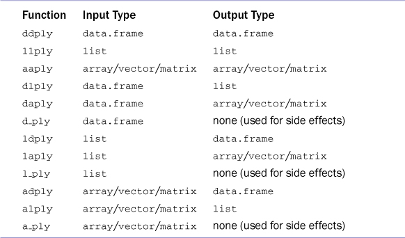
One of the best things to ever happen to R was the development of the plyr4 package by Hadley Wickham. It epitomizes the “split-apply-combine” method of data manipulation. The core of plyr consists of functions such as ddply, llply and ldply. All of the manipulation functions consist of five letters, with the last three always being ply. The first letter indicates the type of input and the second letter indicates the type of output. For instance, ddply takes in a data.frame and outputs a data.frame, llply takes in a list and outputs a list and ldply takes in a list and outputs a data.frame. A full enumeration is listed in Table 11.1.
4. A play on the word plier because it is one of the most versatile and essential tools.
11.3.1. ddply
ddply takes a data.frame, splits it according to some variable(s), performs a desired action on it and returns a data.frame. To learn about ddply we look at the baseball data that come with plyr.
> require(plyr)
> head(baseball)
id year stint team lg g ab r h X2b X3b hr rbi sb cs bb
4 ansonca01 1871 1 RC1 25 120 29 39 11 3 0 16 6 2 2
44 forceda01 1871 1 WS3 32 162 45 45 9 4 0 29 8 0 4
68 mathebo01 1871 1 FW1 19 89 15 24 3 1 0 10 2 1 2
99 startjo01 1871 1 NY2 33 161 35 58 5 1 1 34 4 2 3
102 suttoez01 1871 1 CL1 29 128 35 45 3 7 3 23 3 1 1
106 whitede01 1871 1 CL1 29 146 40 47 6 5 1 21 2 2 4
so ibb hbp sh sf gidp
4 1 NA NA NA NA NA
44 0 NA NA NA NA NA
68 0 NA NA NA NA NA
99 0 NA NA NA NA NA
102 0 NA NA NA NA NA
106 1 NA NA NA NA NA
A common statistic in baseball is On Base Percentage (OBP), which is calculated as
where
H = Hits
BB = Bases on Balls (Walks)
HBP = Times Hit by Pitch
AB = At Bats
SF = Sacrifice Flies
Before 1954 sacrifice flies were counted as part of sacrifice hits, which includes bunts, so for players before 1954 sacrifice flies should be assumed to be 0. That will be the first change we make to the data. There are many instances of HBP (hit by pitch) that are NA, so we set those to 0 as well. We also exclude players with less than 50 at bats in a season.
> # subsetting with [ is faster than using ifelse
> baseball$sf[baseball$year < 1954] <- 0
> # check that it worked
> any(is.na(baseball$sf))
[1] FALSE
> # set NA hbp's to 0
> baseball$hbp[is.na(baseball$hbp)] <- 0
> # check that it worked
> any(is.na(baseball$hbp))
[1] FALSE
> # only keep players with at least 50 at bats in a season
> baseball <- baseball[baseball$ab >= 50, ]
Calculating the OBP for a given player in a given year is easy enough with just vector operations.
> # calculate OBP
> baseball$OBP <- with(baseball, (h + bb + hbp)/(ab + bb + hbp + sf))
> tail(baseball)
id year stint team lg g ab r h X2b X3b hr rbi sb
89499 claytro01 2007 1 TOR AL 69 189 23 48 14 0 1 12 2
89502 cirilje01 2007 1 MIN AL 50 153 18 40 9 2 2 21 2
89521 bondsba01 2007 1 SFN NL 126 340 75 94 14 0 28 66 5
89523 biggicr01 2007 1 HOU NL 141 517 68 130 31 3 10 50 4
89530 ausmubr01 2007 1 HOU NL 117 349 38 82 16 3 3 25 6
89533 aloumo01 2007 1 NYN NL 87 328 51 112 19 1 13 49 3
cs bb so ibb hbp sh sf gidp OBP
89499 1 14 50 0 1 3 3 8 0.3043478
89502 0 15 13 0 1 3 2 9 0.3274854
89521 0 132 54 43 3 0 2 13 0.4800839
89523 3 23 112 0 3 7 5 5 0.2846715
89530 1 37 74 3 6 4 1 11 0.3180662
89533 0 27 30 5 2 0 3 13 0.3916667
Here we used a new function, with. This allows us to specify the columns of a data.frame without having to specify the data.frame name each time.
To calculate the OBP for a player’s entire career we cannot just average his individual season OBPs; we need to calculate and sum the numerator, and then divide by the sum of the denominator. This requires the use of ddply.
First we make a function to do that calculation, then we use ddply to run that calculation for each player.
> # this function assumes that the column names for the data are as
> # below
> obp <- function(data)
+ {
+ c(OBP = with(data, sum(h + bb + hbp)/sum(ab + bb + hbp + sf)))
+ }
>
> # use ddply to calculate career OBP for each player
> careerOBP <- ddply(baseball, .variables = "id", .fun = obp)
> # sort the results by OBP
> careerOBP <- careerOBP[order(careerOBP$OBP, decreasing = TRUE), ]
> # see the results
> head(careerOBP, 10)
id OBP
1089 willite01 0.4816861
875 ruthba01 0.4742209
658 mcgrajo01 0.4657478
356 gehrilo01 0.4477848
85 bondsba01 0.4444622
476 hornsro01 0.4339068
184 cobbty01 0.4329655
327 foxxji01 0.4290509
953 speaktr01 0.4283386
191 collied01 0.4251246
This nicely returns the top ten players by career on base percentage. Notice that Billy Hamilton and Bill Joyce are absent from our results because they are mysteriously missing from the baseball data.
11.3.2. llply
In Section 11.1.2 we use lapply to sum each element of a list.
> theList <- list(A = matrix(1:9, 3), B = 1:5, C = matrix(1:4, 2), D = 2)
> lapply(theList, sum)
$A
[1] 45
$B
[1] 15
$C
[1] 10
$D
[1] 2
This can be done with llpply, yielding identical results.
> llply(theList, sum)
$A
[1] 45
$B
[1] 15
$C
[1] 10
$D
[1] 2
> identical(lapply(theList, sum), llply(theList, sum))
[1] TRUE
To get the result as a vector, laply can be used similarly to sapply.
> sapply(theList, sum)
A B C D
45 15 10 2
> laply(theList, sum)
[1] 45 15 10 2
Notice, however, that while the results are the same, laply did not include names for the vector. These little nuances can be maddening but help dictate when to use which function.
11.3.3. plyr Helper Functions
plyr has a great deal of useful helper functions such as each, which lets us supply multiple functions to a function like aggregate.
> aggregate(price ~ cut, diamonds, each(mean, median))
cut price.mean price.median
1 Fair 4358.758 3282.000
2 Good 3928.864 3050.500
3 Very Good 3981.760 2648.000
4 Premium 4584.258 3185.000
5 Ideal 3457.542 1810.000
Another great function is idata.frame, which creates a reference to a data.frame so that subsetting is much faster and more memory efficient. To illustrate this, we do a simple operation on the baseball data with the regular data.frame and an idata.frame.
> system.time(dlply(baseball, "id", nrow))
user system elapsed
0.29 0.00 0.33
> iBaseball <- idata.frame(baseball)
> system.time(dlply(iBaseball, "id", nrow))
user system elapsed
0.42 0.00 0.47
While saving less than a second in run time might seem trivial the savings can really add up with more complex operations, bigger data, more groups to split by and repeated operation.
11.3.4. Speed versus Convenience
A criticism often leveled at plyr is that it can run slowly. The typical response to this is that using plyr is a question of speed versus convenience. Most of the functionality in plyr can be accomplished using base functions or other packages, but few of those offer the ease of use of plyr. That said, in recent years Hadley Wickham has taken great steps to speed up plyr, including optimized R code, C++ code and parallelization.
11.4. data.table
For speed junkies there is a package called data.table that extends and enhances the functionality of data.frames. The syntax is a little different from regular data.frames, so it will take getting used to, which is probably the primary reason it has not seen near-universal adoption.
The secret to the speed is that data.tables have an index like databases. This allows faster value accessing, group by operations and joins.
Creating data.tables is just like creating data.frames, and the two are very similar.
> require(data.table)
> # create a regular data.frame
> theDF <- data.frame(A=1:10,
+ B=letters[1:10],
+ C=LETTERS[11:20],
+ D=rep(c("One", "Two", "Three"), length.out=10))
> # create a data.table
> theDT <- data.table(A=1:10,
+ B=letters[1:10],
+ C=LETTERS[11:20],
+ D=rep(c("One", "Two", "Three"), length.out=10))
> # print them and compare
> theDF
A B C D
1 1 a K One
2 2 b L Two
3 3 c M Three
4 4 d N One
5 5 e O Two
6 6 f P Three
7 7 g Q One
8 8 h R Two
9 9 i S Three
10 10 j T One
> theDT
A B C D
1: 1 a K One
2: 2 b L Two
3: 3 c M Three
4: 4 d N One
5: 5 e O Two
6: 6 f P Three
7: 7 g Q One
8: 8 h R Two
9: 9 i S Three
10: 10 j T One
> # notice by default data.frame turns character data into factors
> # while data.table does not
> class(theDF$B)
[1] "factor"
> class(theDT$B)
[1] "character"
The data are identical—except that data.frame turned B into a factor while data.table did not—and only the way it was printed looks different.
It is also possible to create a data.table out of an existing data.frame.
> diamondsDT <- data.table(diamonds)
> diamondsDT
carat cut color clarity depth table price x y z
1: 0.23 Ideal E SI2 61.5 55 326 3.95 3.98 2.43
2: 0.21 Premium E SI1 59.8 61 326 3.89 3.84 2.31
3: 0.23 Good E VS1 56.9 65 327 4.05 4.07 2.31
4: 0.29 Premium I VS2 62.4 58 334 4.20 4.23 2.63
5: 0.31 Good J SI2 63.3 58 335 4.34 4.35 2.75
---
53936: 0.72 Ideal D SI1 60.8 57 2757 5.75 5.76 3.50
53937: 0.72 Good D SI1 63.1 55 2757 5.69 5.75 3.61
53938: 0.70 Very Good D SI1 62.8 60 2757 5.66 5.68 3.56
53939: 0.86 Premium H SI2 61.0 58 2757 6.15 6.12 3.74
53940: 0.75 Ideal D SI2 62.2 55 2757 5.83 5.87 3.64
Notice that printing the diamonds data would try to print out all the data but data.table intelligently just prints the first five and last five rows.
Accessing rows can be done similarly to accessing rows in a data.frame.
> theDT[1:2, ]
A B C D
1: 1 a K One
2: 2 b L Two
> theDT[theDT$A >= 7, ]
A B C D
1: 7 g Q One
2: 8 h R Two
3: 9 i S Three
4: 10 j T One
While the second line in the preceding code is valid syntax, it is not necessarily efficient syntax. That line creates a vector of length nrow(theDT)=10 consisting of TRUE or FALSE entries, which is a vector scan. After we create a key for the data.table we can use different syntax to pick rows through a binary search, which will be much faster and is covered in Section 11.4.1.
Accessing individual columns must be done a little differently than accessing columns in data.frames. In Section 5.1 we show that multiple columns in a data.frame should be specified as a character vector. With data.tables the columns should be specified as a list of the actual names, not as characters.
> theDT[, list(A, C)]
A C
1: 1 K
2: 2 L
3: 3 M
4: 4 N
5: 5 O
6: 6 P
7: 7 Q
8: 8 R
9: 9 S
10: 10 T
> # just one column
> theDT[, B]
[1] "a" "b" "c" "d" "e" "f" "g" "h" "i" "j"
> # one column while maintaining data.table structure
> theDT[, list(B)]
B
1: a
2: b
3: c
4: d
5: e
6: f
7: g
8: h
9: i
10: j
If we must specify the column names as characters (perhaps because they were passed as arguments to a function), the with argument should be set to FALSE.
> theDT[, "B", with = FALSE]
B
1: a
2: b
3: c
4: d
5: e
6: f
7: g
8: h
9: i
10: j
> theDT[, c("A", "C"), with = FALSE]
A C
1: 1 K
2: 2 L
3: 3 M
4: 4 N
5: 5 O
6: 6 P
7: 7 Q
8: 8 R
9: 9 S
10: 10 T
This time we used a vector to hold the column names instead of a list. These nuances are important to proper functions of data.tables but can lead to a great deal of frustration.
11.4.1. Keys
Now that we have a few data.tables in memory, we might be interested in seeing some information about them.
> # show tables
> tables()
NAME NROW MB
[1,] diamondsDT 53,940 4
[2,] theDT 10 1
COLS KEY
[1,] carat,cut,color,clarity,depth,table,price,x,y,z
[2,] A,B,C,D
Total: 5MB
This shows, for each data.table in memory, the name, the number of rows, the size in megabytes, the column names and the key. We have not assigned keys for any of the tables so that column is blank. The key is used to index the data.table and will provide the extra speed.
We start by adding a key to theDT. We will use the D column to index the data.table. This is done using setkey, which takes the name of the data.table as its first argument and the name of the desired column (without quotes, as is consistent with column selection) as the second argument.
> # set the key
> setkey(theDT, D)
> # show the data.table again
> theDT
A B C D
1: 1 a K One
2: 4 d N One
3: 7 g Q One
4: 10 j T One
5: 3 c M Three
6: 6 f P Three
7: 9 i S Three
8: 2 b L Two
9: 5 e O Two
10: 8 h R Two
The data have been reordered according to column D, which is sorted alphabetically.
We can confirm the key was set with key.
> key(theDT)
[1] "D"
Or tables.
> tables()
NAME NROW MB
[1,] diamondsDT 53,940 4
[2,] theDT 10 1
COLS KEY
[1,] carat,cut,color,clarity,depth,table,price,x,y,z
[2,] A,B,C,D D
Total: 5MB
This adds some new functionality to selecting rows from data.tables. In addition to selecting rows by the row number or by some expression that evaluates to TRUE or FALSE, a value of the key column can be specified.
> theDT["One", ]
D A B C
1: One 1 a K
2: One 4 d N
3: One 7 g Q
4: One 10 j T
> theDT[c("One", "Two"), ]
D A B C
1: One 1 a K
2: One 4 d N
3: One 7 g Q
4: One 10 j T
5: Two 2 b L
6: Two 5 e O
7: Two 8 h R
More than one column can be set as the key.
> # set the key
> setkey(diamondsDT, cut, color)
To access rows according to both keys, there is a special function named J. It takes multiple arguments, each of which is a vector of values to select.
> # access some rows
> diamondsDT[J("Ideal", "E"), ]
cut color carat clarity depth table price x y z
1: Ideal E 0.23 SI2 61.5 55 326 3.95 3.98 2.43
2: Ideal E 0.26 VVS2 62.9 58 554 4.02 4.06 2.54
3: Ideal E 0.70 SI1 62.5 57 2757 5.70 5.72 3.57
4: Ideal E 0.59 VVS2 62.0 55 2761 5.38 5.43 3.35
5: Ideal E 0.74 SI2 62.2 56 2761 5.80 5.84 3.62
---
3899: Ideal E 0.70 SI1 61.7 55 2745 5.71 5.74 3.53
3900: Ideal E 0.51 VVS1 61.9 54 2745 5.17 5.11 3.18
3901: Ideal E 0.56 VVS1 62.1 56 2750 5.28 5.29 3.28
3902: Ideal E 0.77 SI2 62.1 56 2753 5.84 5.86 3.63
3903: Ideal E 0.71 SI1 61.9 56 2756 5.71 5.73 3.54
> diamondsDT[J("Ideal", c("E", "D")), ]
cut color carat clarity depth table price x y z
1: Ideal E 0.23 SI2 61.5 55 326 3.95 3.98 2.43
2: Ideal E 0.26 VVS2 62.9 58 554 4.02 4.06 2.54
3: Ideal E 0.70 SI1 62.5 57 2757 5.70 5.72 3.57
4: Ideal E 0.59 VVS2 62.0 55 2761 5.38 5.43 3.35
5: Ideal E 0.74 SI2 62.2 56 2761 5.80 5.84 3.62
---
6733: Ideal D 0.51 VVS2 61.7 56 2742 5.16 5.14 3.18
6734: Ideal D 0.51 VVS2 61.3 57 2742 5.17 5.14 3.16
6735: Ideal D 0.81 SI1 61.5 57 2748 6.00 6.03 3.70
6736: Ideal D 0.72 SI1 60.8 57 2757 5.75 5.76 3.50
6737: Ideal D 0.75 SI2 62.2 55 2757 5.83 5.87 3.64
11.4.2. data.table Aggregation
The primary benefit of indexing is faster aggregation. While aggregate and the various d*ply functions will work because data.tables are just enhanced data.frames, they will be slower than using the built-in aggregation functionality of data.table.
In Section 11.2 we calculate the mean price of diamonds for each type of cut.
> aggregate(price ~ cut, diamonds, mean)
cut price
1 Fair 4358.758
2 Good 3928.864
3 Very Good 3981.760
4 Premium 4584.258
5 Ideal 3457.542
To get the same result using data.table, we do this:
> diamondsDT[, mean(price), by = cut]
cut V1
1: Fair 4358.758
2: Good 3928.864
3: Very Good 3981.760
4: Premium 4584.258
5: Ideal 3457.542
The only difference between this and the previous result is that the columns have different names. To specify the name of the resulting column, pass the aggregation function as a named list.
> diamondsDT[, list(price = mean(price)), by = cut]
cut price
1: Fair 4358.758
2: Good 3928.864
3: Very Good 3981.760
4: Premium 4584.258
5: Ideal 3457.542
To aggregate on multiple columns, specify them as a list().
> diamondsDT[, mean(price), by = list(cut, color)]
cut color V1
1: Fair D 4291.061
2: Fair E 3682.312
3: Fair F 3827.003
4: Fair G 4239.255
5: Fair H 5135.683
6: Fair I 4685.446
7: Fair J 4975.655
8: Good D 3405.382
9: Good E 3423.644
10: Good F 3495.750
11: Good G 4123.482
12: Good H 4276.255
13: Good I 5078.533
14: Good J 4574.173
15: Very Good D 3470.467
16: Very Good E 3214.652
17: Very Good F 3778.820
18: Very Good G 3872.754
19: Very Good H 4535.390
20: Very Good I 5255.880
21: Very Good J 5103.513
22: Premium D 3631.293
23: Premium E 3538.914
24: Premium F 4324.890
25: Premium G 4500.742
26: Premium H 5216.707
27: Premium I 5946.181
28: Premium J 6294.592
29: Ideal D 2629.095
30: Ideal E 2597.550
31: Ideal F 3374.939
32: Ideal G 3720.706
33: Ideal H 3889.335
34: Ideal I 4451.970
35: Ideal J 4918.186
cut color V1
To aggregate multiple arguments, pass them as a list. Unlike with aggregate, a different metric can be measured for each column.
> diamondsDT[, list(price = mean(price), carat = mean(carat)), by = cut]
cut price carat
1: Ideal 3457.542 0.7028370
2: Premium 4584.258 0.8919549
3: Good 3928.864 0.8491847
4: Very Good 3981.760 0.8063814
5: Fair 4358.758 1.0461366
> diamondsDT[, list(price = mean(price), carat = mean(carat),
+ caratSum = sum(carat)), by = cut]
cut price carat caratSum
1: Ideal 3457.542 0.7028370 15146.84
2: Premium 4584.258 0.8919549 12300.95
3: Good 3928.864 0.8491847 4166.10
4: Very Good 3981.760 0.8063814 9742.70
5: Fair 4358.758 1.0461366 1684.28
Finally, both multiple metrics can be calculated and multiple grouping variables can be specified at the same time.
> diamondsDT[, list(price = mean(price), carat = mean(carat)),
+ by = list(cut, color)]
cut color price carat
1: Ideal E 2597.550 0.5784012
2: Premium E 3538.914 0.7177450
3: Good E 3423.644 0.7451340
4: Premium I 5946.181 1.1449370
5: Good J 4574.173 1.0995440
6: Very Good J 5103.513 1.1332153
7: Very Good I 5255.880 1.0469518
8: Very Good H 4535.390 0.9159485
9: Fair E 3682.312 0.8566071
10: Ideal J 4918.186 1.0635937
11: Premium F 4324.890 0.8270356
12: Ideal I 4451.970 0.9130291
13: Good I 5078.533 1.0572222
14: Very Good E 3214.652 0.6763167
15: Very Good G 3872.754 0.7667986
16: Very Good D 3470.467 0.6964243
17: Very Good F 3778.820 0.7409612
18: Good F 3495.750 0.7759296
19: Good H 4276.255 0.9147293
20: Good D 3405.382 0.7445166
21: Ideal G 3720.706 0.7007146
22: Premium D 3631.293 0.7215471
23: Premium J 6294.592 1.2930941
24: Ideal D 2629.095 0.5657657
25: Premium G 4500.742 0.8414877
26: Premium H 5216.707 1.0164492
27: Fair F 3827.003 0.9047115
28: Ideal F 3374.939 0.6558285
29: Ideal H 3889.335 0.7995249
30: Fair H 5135.683 1.2191749
31: Good G 4123.482 0.8508955
32: Fair G 4239.255 1.0238217
33: Fair J 4975.655 1.3411765
34: Fair I 4685.446 1.1980571
35: Fair D 4291.061 0.9201227
cut color price carat
11.5. Conclusion
Aggregating data is a very important step in the analysis process. Sometimes it is the end goal, and other times it is in preparation for applying more advanced methods. No matter the reason for aggregation, there are plenty of functions to make it possible. These include aggregate, apply and lapply in base; ddply, llply and the rest in plyr; and the group by functionality in data.table.