
4
GENERATING MUSICAL OVERTONES WITH THE KARPLUS-STRONG ALGORITHM

One of the main characteristics of any musical sound is its pitch, or frequency. This is the number of vibrations per second in hertz (Hz). For example, the third string from the top of an acoustic guitar produces an D note with a frequency of 146.83 Hz. This is a sound you can approximate by creating a sine wave with a frequency of 146.83 Hz on a computer, as shown in Figure 4-1.
Unfortunately, if you play this sine wave on your computer, it won’t sound anything like a guitar or a piano. What makes a computer sound so different from a musical instrument when playing the same note?

Figure 4-1: Sine wave at 146.83 Hz
When you pluck a string on the guitar, the instrument produces a mix of frequencies with varying intensity, as shown in the spectral plot in Figure 4-2. The sound is most intense when the note is first struck, and the intensity dies off over time. The dominant frequency you hear when you pluck the D string on the guitar, called the fundamental frequency, is 146.83 Hz, but you also hear certain multiples of that frequency called overtones. The sound of any instrument is comprised of this fundamental frequency and overtones, and it’s the combination of these that makes a guitar sound like a guitar.

Figure 4-2: Spectral plot of note D4 played on guitar
As you can see, to simulate the sound of a plucked string instrument on the computer, you need to be able to generate both the fundamental frequency and the overtones. The trick is to use the Karplus-Strong algorithm.
In this project, you’ll generate five guitar-like notes of a musical scale (a series of related notes) using the Karplus-Strong algorithm. You’ll visualize the algorithm used to generate these notes and save the sounds as WAV files. You’ll also create a way to play them at random and learn how to do the following:
• Implement a ring buffer using the Python deque class.
• Use numpy arrays and ufuncs.
• Play WAV files using pygame.
• Plot a graph using matplotlib.
• Play the pentatonic musical scale.
In addition to implementing the Karplus-Strong algorithm in Python, you’ll also explore the WAV file format and see how to generate notes within a pentatonic musical scale.
How It Works
The Karplus-Strong algorithm can simulate the sound of a plucked string by using a ring buffer of displacement values to simulate a string tied down at both ends, similar to a guitar string.
A ring buffer (also known as a circular buffer) is a fixed-length buffer (just an array of values) that wraps around itself. In other words, when you reach the end of the buffer, the next element you access will be the first element in the buffer. (See “Implementing the Ring Buffer with deque” on page 61 for more about ring buffers.)
The length (N) of the ring buffer is related to the fundamental frequency of vibration according to the equation N = S/f, where S is the sampling rate and f is the frequency.
At the start of the simulation, the buffer is filled with random values in the range [−0.5, 0.5], which you might think of as representing the random displacement of a plucked string as it vibrates.
In addition to the ring buffer, you use a samples buffer to store the intensity of the sound at any particular time. The length of this buffer and the sampling rate determine the length of the sound clip.
The Simulation
The simulation proceeds until the sample buffer is filled in a kind of feedback scheme, as shown in Figure 4-3. For each step of the simulation, you do the following:
1. Store the first value from the ring buffer in the samples buffer.
2. Calculate the average of the first two elements in the ring buffer.
3. Multiply this average value by an attenuation factor (in this case, 0.995).
4. Append this value to the end of the ring buffer.
5. Remove the first element of the ring buffer.
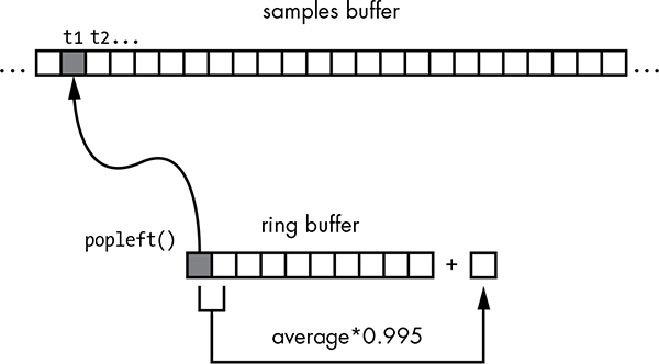
Figure 4-3: Ring buffer and the Karplus-Strong algorithm
To simulate a plucked string, fill a ring buffer with numbers that represent the energy of the wave. The sample buffer, which represents the final sound data, is created by iterating through the values in the ring buffer. Use an averaging scheme (explained in a moment) to update values in the ring buffer.
This feedback scheme is designed to simulate the energy traveling through a vibrating string. According to physics, for a vibrating string, the fundamental frequency is inversely proportional to its length. Since we are interested in generating sounds of a certain frequency, we choose a ring buffer length that is inversely proportional to that frequency. The averaging that happens in step 1 of the simulation acts as a low-pass filter that cuts off higher frequencies and allows lower frequencies through, thereby eliminating higher harmonics (that is, larger multiples of the fundamental frequency) because you’re mainly interested in the fundamental frequency. Finally, you use the attenuation factor to simulate the loss of energy as the wave travels back and forth along the string.
The samples buffer that you use in step 1 of the simulation represents the amplitude of the generated sound over time. To calculate the amplitude at any given time, you update the ring buffer by calculating the average of its first two elements and multiplying the result by an attenuation factor. This calculated value is then appended to the end of the ring buffer, and the first element is removed.
Now let’s look at a simple example of the algorithm in action. The following table represents a ring buffer at two consecutive time steps. Each value in the ring buffer represents the amplitude of the sound. The buffer has five elements, and they are initially filled with some numbers.
Time step 1 |
0.1 |
–0.2 |
0.3 |
0.6 |
–0.5 |
Time step 2 |
–0.2 |
0.3 |
0.6 |
–0.5 |
–0.199 |
As you go from time step 1 to step 2, apply the Karplus-Strong algorithm as follows. The first value in the first row, 0.1, is removed, and all subsequent values from time step 1 are added in the same order to the second row, which represents time step 2. The last value in time step 2 is the attenuated average of the first and last values of time step 1, which is calculated as 0.995 × ((0.1 + –0.5) ÷ 2) = –0.199.
Creating WAV Files
The Waveform Audio File Format (WAV) is used to store audio data. This format is convenient for small audio projects because it is simple and doesn’t require you to deal with complicated compression techniques.
In its simplest form, WAV files consist of a series of bits representing the amplitude of the recorded sound at a given point in time, called the resolution. You’ll use 16-bit resolution in this project. WAV files also have a set sampling rate, which is the number of times the audio is sampled, or read, every second. In this project, you use a sampling rate of 44,100 Hz, the rate used in audio CDs. Let’s generate a five-second audio clip of a 220 Hz sine wave using Python. First, you represent a sine wave using this formula:
A = sin(2πft)
Here, A is the amplitude of the wave, f is the frequency, and t is the current time index. Now you rewrite this equation as follows:
A = sin(2πfi/R)
In this equation, i is the index of the sample, and R is the sampling rate. Using these two equations, you can create a WAV file for a 200 Hz sine wave as follows:
   import numpy as np
   import wave, math

   sRate = 44100
   nSamples = sRate * 5
➊ x = np.arange(nSamples)/float(sRate)
➋ vals = np.sin(2.0*math.pi*220.0*x)
➌ data = np.array(vals*32767, 'int16').tostring()
  file = wave.open('sine220.wav', 'wb')
➍ file.setparams((1, 2, sRate, nSamples, 'NONE', 'uncompressed'))
  file.writeframes(data)
  file.close()
At ➊ and ➋, you create a numpy array (see Chapter 1) of amplitude values, according to the second sine wave equation. The numpy array is a fast and convenient way to apply functions to arrays such as the sin() function.
At ➌, the computed sine wave values in the range [–1, 1] are scaled to 16-bit values and converted to a string so they can be written to a file. At ➍, you set the parameters for the WAV file; in this case, it’s a single-channel (mono), two-byte (16-bit), uncompressed format. Figure 4-4 shows the generated sine220.wav file in Audacity, a free audio editor. As expected, you see a sine wave of frequency 220 Hz, and when you play the file, you hear a 220 Hz tone for five seconds.

Figure 4-4: A sine wave at 220 Hz
The Minor Pentatonic Scale
A musical scale is a series of notes in increasing or decreasing pitch or frequency. A musical interval is the difference between two pitches. Usually, all notes in a piece of music are chosen from a particular scale. A semitone is a basic building block of a scale and is the smallest musical interval in Western music. A tone is twice the length of a semitone. The major scale, one of the most common musical scales, is defined by the interval pattern tone-tone-semitone-tone-tone-tone-semitone.
We will briefly go into the pentatonic scale here, since we want to generate musical notes in that scale. This section will tell you how we came up with the frequency numbers used by our program to generate these notes using the Karplus-Strong algorithm. The pentatonic scale is a five-note musical scale. For example, the famous American song “Oh! Susanna” is based on a pentatonic scale. A variant of this scale is the minor pentatonic scale.
This scale is given by the note sequence (tone+semitone)-tone-tone-(tone+semitone)-tone. Thus, the C minor pentatonic scale consists of the notes C, E-flat, F, G, and B-flat. Table 4-1 lists the frequencies of the five notes of a minor pentatonic scale that you will generate using the Karplus-Strong algorithm. (Here, C4 designates C in the fourth octave of a piano, or middle C, by convention.)
Table 4-1: Notes in a Minor Pentatonic Scale
Note |
Frequency (Hz) |
C4 |
261.6 |
E-flat |
311.1 |
F |
349.2 |
G |
392.0 |
B-flat |
466.2 |
Requirements
In this project, you’ll use the Python wave module to create audio files in WAV format. You’ll use numpy arrays for the Karplus-Strong algorithm and the deque class from Python collections to implement the ring buffer. You’ll also play back the WAV files with the pygame module.
The Code
Now let’s develop the various pieces of code required to implement the Karplus-Strong algorithm and then put them together for the complete program. To see the full project code, skip ahead to “The Complete Code” on page 65.
Implementing the Ring Buffer with deque
Recall from earlier that the Karplus-Strong algorithm uses a ring buffer to generate a musical note. You’ll implement the ring buffer using Python’s deque container (pronounced “deck”)—part of Python’s collections module—which provides specialized container data types in an array. You can insert and remove elements from the beginning (head) or end (tail) of a deque (see Figure 4-5). This insertion and removal process is a O(1), or a “constant time” operation, which means it takes the same amount of time regardless of how big the deque container gets.

Figure 4-5: Ring buffer using deque
The following code shows how you would use deque in Python:
   >>> from collections import deque
➊  >>> d = deque(range(10))
   >>> print(d)
   deque([0, 1, 2, 3, 4, 5, 6, 7, 8, 9])
➋  >>> d.append(-1)
   >>> print(d)
   deque([0, 1, 2, 3, 4, 5, 6, 7, 8, 9, -1])
➌  >>> d.popleft()
   0
   >>> print d
   deque([1, 2, 3, 4, 5, 6, 7, 8, 9, -1])
At ➊, you create the deque container by passing in a list created by the range() method. At ➋, you append an element to the end of the deque container, and at ➌, you pop (remove) the first element from the head of the deque. Both these operations happen quickly.
Implementing the Karplus-Strong Algorithm
You also use a deque container to implement the Karplus-Strong algorithm for the ring buffer, as shown here:
   # generate note of given frequency
   def generateNote(freq):
       nSamples = 44100
       sampleRate = 44100
       N = int(sampleRate/freq)
       # initialize ring buffer
➊      buf = deque([random.random() - 0.5 for i in range(N)])
       # initialize samples buffer
➋      samples = np.array([0]*nSamples, 'float32')
       for i in range(nSamples):
➌          samples[i] = buf[0]
➍          avg = 0.996*0.5*(buf[0] + buf[1])
           buf.append(avg)
           buf.popleft()

       # convert samples to 16-bit values and then to a string
       # the maximum value is 32767 for 16-bit
➎     samples = np.array(samples*32767, 'int16')
➏     return samples.tostring()
At ➊, you initialize deque with random numbers in the range [–0.5, 0.5]. At ➋, you set up a float array to store the sound samples. The length of this array matches the sampling rate, which means the sound clip will be generated for one second.
The first element in deque is copied to the samples buffer at ➌. At ➍, and in the lines that follow, you can see the low-pass filter and attenuation in action. At ➎, the samples array is converted into a 16-bit format by multiplying each value by 32,767 (a 16-bit signed integer can take only values from −32,768 to 32,767), and at ➏, it is converted to a string representation for the wave module, which you’ll use to save this data to a file.
Writing a WAV File
Once you have the audio data, you can write it to a WAV file using the Python wave module.
   def writeWAVE(fname, data):
       # open file
➊     file = wave.open(fname, 'wb')
       # WAV file parameters
       nChannels = 1
       sampleWidth = 2
       frameRate = 44100
       nFrames = 44100
       # set parameters
➋     file.setparams((nChannels, sampleWidth, frameRate, nFrames,
                       'NONE', 'noncompressed'))

➌     file.writeframes(data)
       file.close()
At ➊, you create a WAV file, and at ➋, you set its parameters using a single-channel, 16-bit, uncompressed format. Finally, at ➌, you write the data to the file.
Playing WAV Files with pygame
Now you’ll use the Python pygame module to play the WAV files generated by the algorithm. pygame is a popular Python module used to write games. It’s built on top of the Simple DirectMedia Layer (SDL) library, a high-performance, low-level library that gives you access to sound, graphics, and input devices on a computer.
For convenience, you encapsulate the code in a NotePlayer class, as shown here:
   # play a WAV file
   class NotePlayer:
       # constructor
       def __init__(self):
➊         pygame.mixer.pre_init(44100, -16, 1, 2048)
           pygame.init()
           # dictionary of notes
➋         self.notes = {}
    # add a note
    def add(self, fileName):
➌      self.notes[fileName] = pygame.mixer.Sound(fileName)
    # play a note
    def play(self, fileName):
        try:
➍          self.notes[fileName].play()
        except:
            print(fileName + ' not found!')
    def playRandom(self):
        """play a random note"""
➎      index = random.randint(0, len(self.notes)-1)
➏      note = list(self.notes.values())[index]
        note.play()
At ➊, you preinitialize the pygame mixer class with a sampling rate of 44,100, 16-bit signed values, a single channel, and a buffer size of 2,048. At ➋, you create a dictionary of notes, which stores the pygame sound objects against the filenames. Next, in NotePlayer’s add() method ➌, you create the sound object and store it in the notes dictionary.
Notice in play() how the dictionary is used at ➍ to select and play the sound object associated with a filename. The playRandom() method picks a random note from the five notes you’ve generated and plays it. Finally, at ➎, randint() selects a random integer from the range [0, 4] and at ➏ picks a note to play from the dictionary.
The main() Method
Now let’s look at the main() method, which creates the notes and handles various command line options to play the notes.
   parser = argparse.ArgumentParser(description="Generating sounds with
       Karplus String Algorithm")
   # add arguments
➊ parser.add_argument('--display', action='store_true', required=False)
   parser.add_argument('--play', action='store_true', required=False)
   parser.add_argument('--piano', action='store_true', required=False)
   args = parser.parse_args()

   # show plot if flag set
   if args.display:
       gShowPlot = True
       plt.ion()

   # create note player
   nplayer = NotePlayer()

   print('creating notes...')
   for name, freq in list(pmNotes.items()):
       fileName = name + '.wav'
➋     if not os.path.exists(fileName) or args.display:
           data = generateNote(freq)
           print('creating ' + fileName + '...')
           writeWAVE(fileName, data)
       else:
           print('fileName already created. skipping...')

       # add note to player
➌     nplayer.add(name + '.wav')

       # play note if display flag set
       if args.display:
➍         nplayer.play(name + '.wav')
           time.sleep(0.5)

   # play a random tune
   if args.play:
       while True:
           try:
➎             nplayer.playRandom()
               # rest - 1 to 8 beats
➏             rest = np.random.choice([1, 2, 4, 8], 1,
                                       p=[0.15, 0.7, 0.1, 0.05])
               time.sleep(0.25*rest[0])
           except KeyboardInterrupt:
               exit()
First, you set up some command line options for the program using argparse, as discussed in earlier projects. At ➊, if the --display command line option was used, you set up a matplotlib plot to show how the waveform evolves during the Karplus-Strong algorithm. The ion() call enables interactive mode for matplotlib. You then create an instance of the NotePlayer class, generating the notes in a pentatonic scale using the generateNote() method. The frequencies for the five notes are defined in the global dictionary pmNotes.
At ➋, you use the os.path.exists() method to see whether the WAV file has been created. If so, you skip the computation. (This is a handy optimization if you’re running this program several times.)
Once the note is computed and the WAV file created, you add the note to the NotePlayer dictionary at ➌ and then play it at ➍ if the display command line option is used.
At ➎, if the –play option is used, the playRandom() method in NotePlayer plays a note at random from the five notes. For a note sequence to sound even remotely musical, you need to add rests between the notes played, so you use the random.choice() method from numpy at ➏ to choose a random rest interval. This method also lets you choose the probability of the rest interval, which you set so that a two-beat rest is the most probable and an eight-beat rest the least probable. Try changing these values to create your own style of random music!
The Complete Code
Now let’s put the program together. The complete code is shown here and can also be downloaded from https://github.com/electronut/pp/blob/master/karplus/ks.py.
import sys, os
import time, random
import wave, argparse, pygame
import numpy as np
from collections import deque
from matplotlib import pyplot as plt

# show plot of algorithm in action?
gShowPlot = False

# notes of a Pentatonic Minor scale
# piano C4-E(b)-F-G-B(b)-C5
pmNotes = {'C4': 262, 'Eb': 311, 'F': 349, 'G':391, 'Bb':466}

# write out WAV file
def writeWAVE(fname, data):
    # open file
    file = wave.open(fname, 'wb')
    # WAV file parameters
    nChannels = 1
    sampleWidth = 2
    frameRate = 44100
    nFrames = 44100

    # set parameters
    file.setparams((nChannels, sampleWidth, frameRate, nFrames,
                    'NONE', 'noncompressed'))
    file.writeframes(data)
    file.close()

# generate note of given frequency
def generateNote(freq): nSamples = 44100
    sampleRate = 44100
    N = int(sampleRate/freq)
    # initialize ring buffer
    buf = deque([random.random() - 0.5 for i in range(N)])
    # plot of flag set
    if gShowPlot:
        axline, = plt.plot(buf)
    # initialize samples buffer
    samples = np.array([0]*nSamples, 'float32')
    for i in range(nSamples):
        samples[i] = buf[0]
        avg = 0.995*0.5*(buf[0] + buf[1])
        buf.append(avg)
        buf.popleft()
        # plot of flag set
        if gShowPlot:
            if i % 1000 == 0:
                axline.set_ydata(buf)
                plt.draw()

    # convert samples to 16-bit values and then to a string
    # the maximum value is 32767 for 16-bit
    samples = np.array(samples*32767, 'int16')
    return samples.tostring()

# play a WAV file
class NotePlayer:
    # constructor
    def __init__(self):
        pygame.mixer.pre_init(44100, -16, 1, 2048)
        pygame.init()
        # dictionary of notes
        self.notes = {}
    # add a note
    def add(self, fileName):
        self.notes[fileName] = pygame.mixer.Sound(fileName)
    # play a note
    def play(self, fileName):
        try:
            self.notes[fileName].play()
        except:
            print(fileName + ' not found!')
    def playRandom(self):
        """play a random note"""
        index = random.randint(0, len(self.notes)-1)

        note = list(self.notes.values())[index]
        note.play()
# main() function
def main():
    # declare global var
    global gShowPlot

    parser = argparse.ArgumentParser(description="Generating sounds with
        Karplus String Algorithm")
    # add arguments
    parser.add_argument('--display', action='store_true', required=False)
    parser.add_argument('--play', action='store_true', required=False)
    parser.add_argument('--piano', action='store_true', required=False)
    args = parser.parse_args()

    # show plot if flag set
    if args.display:
        gShowPlot = True
        plt.ion()

    # create note player
    nplayer = NotePlayer()

    print('creating notes...')
    for name, freq in list(pmNotes.items()):
        fileName = name + '.wav'
        if not os.path.exists(fileName) or args.display:
            data = generateNote(freq)
            print('creating ' + fileName + '...')
            writeWAVE(fileName, data)
        else:
            print('fileName already created. skipping...')

        # add note to player
        nplayer.add(name + '.wav')

        # play note if display flag set
        if args.display:
            nplayer.play(name + '.wav')
            time.sleep(0.5)

    # play a random tune
    if args.play:
        while True:
            try:
                nplayer.playRandom()
                # rest - 1 to 8 beats
                rest = np.random.choice([1, 2, 4, 8], 1,
                                        p=[0.15, 0.7, 0.1, 0.05])
                time.sleep(0.25*rest[0])
            except KeyboardInterrupt:
                exit()

    # random piano mode
    if args.piano:
        while True:
            for event in pygame.event.get():
                if (event.type == pygame.KEYUP):
                    print("key pressed")
                    nplayer.playRandom()
                    time.sleep(0.5)

# call main
if __name__ == '__main__':
    main()
Running the Plucked String Simulation
To run the code for this project, enter this in a command shell:
$ python3 ks.py –display
As you can see in Figure 4-6, the matplotlib plot shows how the Karplus-Strong algorithm converts the initial random displacements to create waves of the desired frequency.

Figure 4-6: Sample run of Karplus-Strong algorithm
Now try playing a random note using this program.
$ python ks.py –play
This should play a random note sequence using the generated WAV files of the pentatonic musical scale.
Summary
In this project, you used the Karplus-Strong algorithm to simulate the sound of plucked strings and played notes from generated WAV files.
Experiments!
Here are some ideas for experiments:
1. Use the techniques you learned in this chapter to create a method that replicates the sound of two strings of different frequencies vibrating together. Remember, the Karplus-Strong algorithm produces sound amplitudes that can be added together (before scaling to 16-bit values for WAV file creation). Now add a time delay between the first and second string plucks.
2. Write a method to read music from a text file and generate musical notes. Then play the music using these notes. You can use a format where the note names are followed by integer rest time intervals, like this: C4 1 F4 2 G4 1 . . . .
3. Add a --piano command line option to the project. When the project is run with this option, the user should be able to press the A, S, D, F, and G keys on a keyboard to play the five musical notes. (Hint: use pygame.event.get and pygame.event.type.)