
To fit the weights in a neural net for a given training set, we first need to define a cost function:

This is very similar to the cost function we used for logistic regression, except that now we are also summing over k output units. The triple summation used in the regularization term looks a bit complicated, but all it is really doing is summing over each of the terms in the parameter matrix, and using this to calculate the regularization. Note that the summation, i, l, and j start at 1, rather than 0; this is to reflect the fact that we do not apply regularization to the bias unit.
Now that we have cost function, we need to work out a way to minimize it. As with gradient descent, we need to compute the partial derivatives to calculate the slope of the cost function. This is done using the back propagation algorithm. It is called back propagation because we begin by calculating the error at the output layer, then calculating the error for each previous layer in turn. We can use these derivatives calculated by the cost function to work out parameter values for each of the units in our neural network. To do this, we need to define an error term:
For this example, let's assume that we have a total of three layers, including the input and output layers. The error at the output layer can be written as follows:
The activation function in the final layer is equivalent to our hypothesis function, and we can use simple vector subtraction to calculate the difference between the values predicted by our hypothesis, and the actual values in our training set. Once we know the error in our output layer, we are able to back propagate to find the error, which is the delta values, in previous layers:

This will calculate the error for layer three. We use the transpose of the parameter vector of the current layer, in this example layer 2, multiplied by the error vector from the forward layer, in this case layer 3. We then use pairwise multiplication, indicated by the * symbol, with the derivative of the activation function, g, evaluated at the input values given by z(3). We can calculate this derivative term by the following:

If you know calculus, it is a fairly straight forward procedure to prove this, but for our purposes, we will not go into it here. As you would expect when we have more than one hidden layer, we can calculate the delta values for each hidden layer in exactly the same way, using the parameter vector, the delta vector for the forward layer, and the derivative of the activation function for the current layer. We do not need to calculate the delta values for layer 1 because these are just the features themselves without any errors. Finally, through a rather complicated mathematical proof that we will not go into here, we can write the derivative of the cost function, ignoring regularization, as follows:

By computing the delta terms using back propagation, we can find these partial derivatives for each of the parameter values. Now, let's see how we apply this to a dataset of training samples. We need to define capital delta, Δ, which is just the matrix of the delta terms and has the dimensions, l:i:j. This will act as an accumulator of the delta values from each node in the neural network, as the algorithm loops through each training sample. Within each loop, it performs the following functions on each training sample:
- It sets the activation functions in the first layer to each value of x, that is, our input features.
- It performs forward propagation on each subsequent layer in turn up to the output layer to calculate the activation functions for each layer.
- It computes the delta values at the output layer and begins the process of back propagation. This is similar to the process we performed in forward propagation, except that it occurs in reverse. So, for our output layer in our 3-layer example, it is demonstrated as follows:

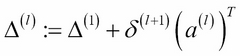
Remember that this is all happening in a loop, so we are dealing with one training sample at a time; y(i) represents the target value of the ith training sample. We can now use the back propagation algorithm to calculate the delta values for previous layers. We can now add these values to the accumulator, using the update rule:
This formula can be expressed in its vectorized form, updating all training samples at once, as shown:
Now, we can add our regularization term:
Finally, we can update the weights by performing gradient descent:
Remember that α is the learning rate, that is, a hyper parameter we set to a small number between 0 and 1.