
![]()
Multiple Regression Analysis
In Chapter 9, we discussed correlation, which is used for quantifying the relation between a pair of variables. We also discussed simple regression, which helps predict the dependent variable when an independent variable is given. In simple regression, you use a single independent variable to predict the dependent variable. This is a simplistic approach, and in practice some dependent variables may require more than one independent variable for accurate predictions. For example, can you predict the gross domestic product (GDP) of a nation by looking just at exports? The obvious answer is that it can’t be done. Predicting the GDP may need several other variables, such as per-capita income, value of natural resources, national debt, and so on. Likewise, the health of an individual depends upon many variables, such as smoking or drinking habits, eating habits, job pressure, daily workouts, genetics, sleeping habits, and more.
In real-life scenarios, you can’t expect a single variable to explain all the variations in a dependent variable; several independent variables are needed to predict most dependent variables in real life. That’s where multiple linear regression analysis comes into the picture. One more classic example of multiple linear regression is the credit risk analysis done by banks, which we have been discussing throughout this book.
Multiple Linear Regression
As discussed, real-world problems are multivariate; in other words, most of the target variables in real life are dependent on multiple independent variables. The overall salary of an employee may depend upon her educational qualifications, years of experience, type and complexity of work, company policies, and so on. Figure 10-1 shows a few more examples.
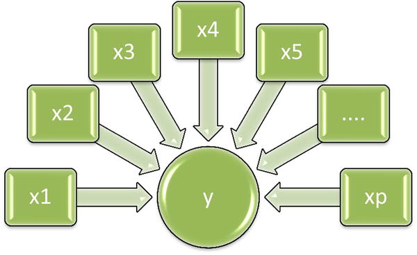
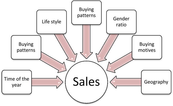

What are the factors that a company should consider for predicting the sales of its product?
What are the factors that a bank should consider to predict the loan-repaying capabilities of its customers?
Most of the economic models to predict profits, return on investments, and so on, involve multiple variables. The multiple regression technique is not very different from that of simple regression models except that multiple variables are involved. The basic assumptions, interpretation of the regression coefficients, and R-square remain the same.
Multiple Regression Line
The simple regression line equation is ![]() . The multiple regression line equation is as follows:
. The multiple regression line equation is as follows:
![]()
where
- β1, β2…….. βp, are the coefficient of x1 x2 …….xp.
- β0 is the intercept.
Here, in multiple regression, your goal is to fit a regression line between all the independent variables and the dependent variable. Consider the example of smartphone sales. Say you want to predict the sales of smartphones using independent variables such as ratings of the phone, price band of the phone, market promotions, and so on.
In a simple regression, you try to fit a regression line between y and x. Since there are only two variables involved in the process, the regression line is a simple straight line on a two-dimensional plot. A straight line involving a regression equation like ![]() will be in three dimensions, as shown in 10-2. It’s obviously harder to imagine than a two-dimensional line involved in a simple linear regression.
will be in three dimensions, as shown in 10-2. It’s obviously harder to imagine than a two-dimensional line involved in a simple linear regression.
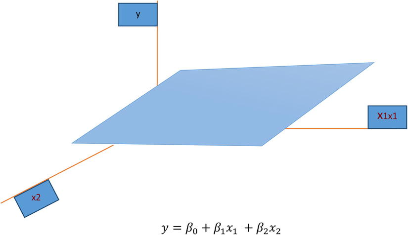
Figure 10-2. Plot for Multiple Regression with Two Independent Variables
In the smartphone sales example, the regression line will look like this:
![]()
Once you have the values of beta coefficients, you can create the regression line equation and use it for predicting the sales. Finding these beta coefficients is the topic of the following sections.
Multiple Regression Line Fitting Using Least Squares
The process of fitting a multiple regression line is the same as the one you studied in Simple regression chapter. The only difference is the number of independent variables and their coefficients. Here you have a number of additional independent variables (x1 x2 …….xp) and you are trying to find multiple coefficients (β1, β2…….. βp).
The following is what you are trying to do:
- Fitting a plane (multidimensional line) that best represents your data
- Fitting a regression line that goes through the most of the points of the data
- Representing the scattered data in the form a multidimensional line with minimal errors
Finding the values of β1, β2…….. βp and β0, the intercept in the equation ![]() Refer to Figure 10-3.
Refer to Figure 10-3.
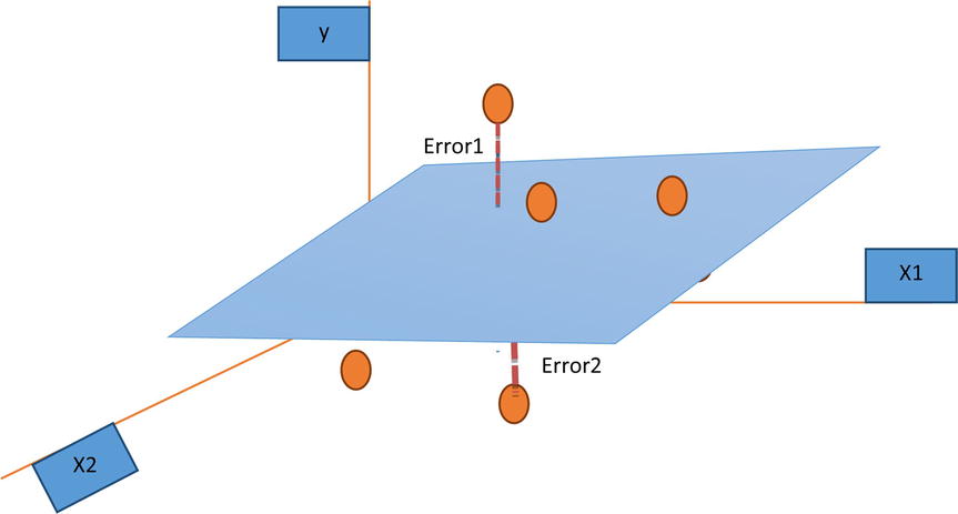
Figure 10-3. Estimated and actual values in regression analysis
Figure 10-3 shows the estimated regression line and the actual values seen in a three-dimensional space. The error is nothing but the distance between the two points. The estimated points on the regression plane and the actual point are denoted as circles. The dotted line is the error. As expected, you always want the difference between the actual value and estimated value to be zero.
Try to minimize the square of the errors to find the beta coefficients.
![]()
![]()
Now you can use optimization techniques to find the values of β1, β2…….. βp and β0 that will minimize the previous function. A line that will result from this procedure will be the best regression line for this data. This is because it makes sure that the sum of squares of errors is kept to the minimum possible value while optimizing.
Multiple Linear Regression in SAS
In SAS you need to mention the data set name and the dependent independent variable list in the model statement. SAS will do the least squares optimization and provide the beta coefficients as the result.
Example: Smartphone Sales Estimation
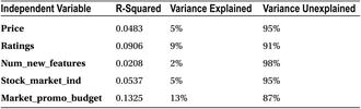
In the smartphone sales example, discussed earlier in Chapter simple regression chapter, you are estimating the sales using independent variables such as Price, Ratings, Num_new_features, Stock_market_ind, and Market_promo_budget. When using variables one at a time, you could not get a good model. The following (Table 10-1) is the R-squared table that shows the variables and variation that they explain in the dependent variable. Please refer to simple regression for mobile phone sales example in the previous chapter.
Table 10-1. R-square table
You now fit a multiple regression line to this problem. The following is the SAS code to do this:
/* Multiple Regression line for Smartphone sales example*/
proc reg data= mobiles;
model sales= Ratings Price Num_new_features Stock_market_ind Market_promo_budget;
run;
Here is the code explanation:
- PROC REG is for calling regression procedure.
- The data set name is mobiles.
- You need to mention the dependent and independent variables in the model statement; sales is the dependent variable.
Table 10-2 shows the SAS output of this code.
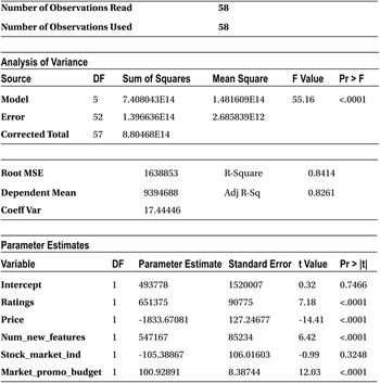
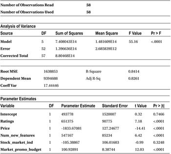
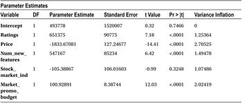
Table 10-2. Output of PROC REG on Mobiles Data Set
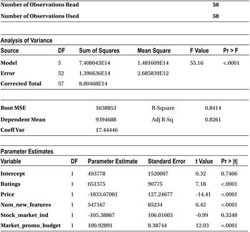
The output has all the regression coefficient estimates. The coefficient of all the independent variables is mentioned against them in the final Parameter Estimates table. The intercept is 493,778. The regression coefficient for ratings is 651,375. For price, it is -1,833.67, and for a number of new features, it stands at 547,167.
The final multiple regression line equation is as follows:

From the previous coefficients and their signs, you can infer that the mobile phone sale number is directly proportional to customer ratings, number of new features added, and market promotion efforts. You can also observe that the sale is inversely proportional to price band and stock market indices (negative coefficient in the regression equation). The relation of stock market index with sales appears slightly against the intuition, but that is what has been happening historically. The stock market index has a negative effect on smartphone sales. If the stock market increases, smartphone sales show a decline, and vice versa for a bearish market.
With this equation, if you have the values of sample ratings, price band, number of new features, stock market indicator, and estimated promotion level of the product, you can get a fair idea about the sales. But unfortunately that’s not all. There are some questions to be answered.
How good is the value of predicted sales? Is this line a good fit to this data? Can you use this regression line for predictions? What is the error or accuracy that you can guarantee using this regression line? How much of the variance in sales is explained by all the variables? How is the goodness of fit measured? Can you use R-squared here as well?
The goodness of fit, or the validation measure, here is R-squared. The R-square value is nothing but the variance explained in the dependent variable by all the variables put together. Multiple regression analysis of variance (ANOVA) tables give the values of the sum of the squares of errors.
Just for your convenience, we have reproduced the analysis of variance tables from the mobile phone sales example in Table 10-3.
Table 10-3. Analysis of Variance Tables from the Mobile Phone Sales Example
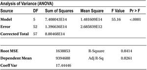
Since the sales numbers are in the millions, the variance (sum of squares) is in multiples of millions. Since all the values are on the same scale, it is easy to interpret the ANOVA table. The total sum of squares or the measure of overall variance in Y is around 8.8 units, whereas the error sum of squares is 1.4 units. The rest is the sum of squares, which is 7.4 units. The R-squared value is 84.14 percent.
Please refer to Chapter 9 on simple regression to learn more about R-square and the sum of squares.
This regression line looks like a fairly accurate model. All the variables together are explaining almost 84 percent of the variation in y (Figure 10-4), though individually none of the variables could explain more than 10 percent of the variation in y. You can confidently go ahead and use this model for predictions.
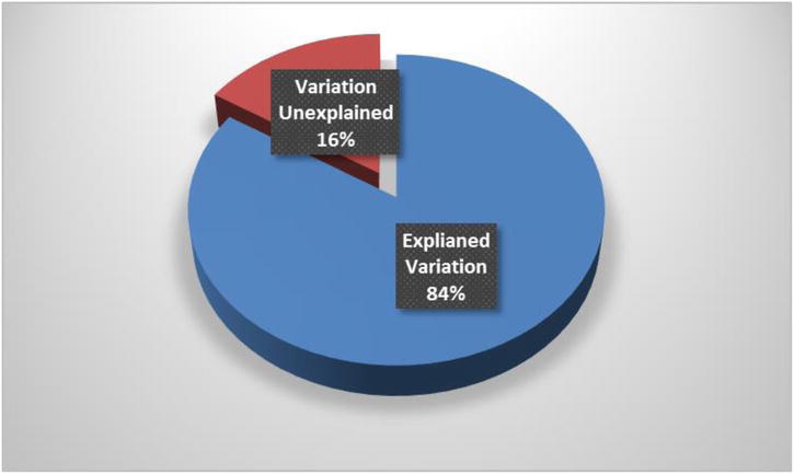
Figure 10-4. Explained and unexplained variations in mobile phone example
Three Main Measures from Regression Output
In the SAS output, you have some other measures also mentioned apart from just the regression coefficients, ANOVA table, and R-square. You may not need to know all of them, but the following are the statistical measures that you must know:
- The F-test, F-value, P-value of F-test
- The T-test, T-value, P-value of T-test
- The R-squared and adjusted R-square
The F-test, F-value, P-value of F-test
You perform the F-test to see whether the model is relevant enough in the current context. This is the test to see the overall fitness of the model. The following questions are answered using this test:
- Is the model relevant at all?
- Is there at least one variable that explains some variation in the dependent variable (y)?
As an example, consider building an analytics model for smartphone sales. Some trivial independent variables such as number of buses in the city, average number of pizzas ordered, and average fuel consumption will definitely not help in predicting the values of smartphone sales. If you use more and more variables like this, the whole model will be irrelevant. The obvious reason is that the independent variables in the model are not able to explain the variation in the dependent variable y. The F-test determines this. It tells whether there is at least one variable in the model that has a significant impact on the dependent variable.
While discussing the multiple regression line earlier in this chapter, we talked about beta coefficients. The F-test uses them to test the explanatory or prediction power of a model. If at least one beta coefficient is not equal to zero, you can infer the presence of one independent variable in the model that has a significant effect on the variation of the dependent variable y. If more than one beta is nonzero, it indicates the presence of multiple independent variables that can explain the variations in y.
H0:
 , which is equivalent to
  .
.- If all betas are zero, it means that the model is insignificant and it has no explanatory prediction power.
H1:
 , which is equivalent to saying that at least one
  .
.
For an explanation of H0 and H1, please refer to Testing of Hypothesis in Chapter 8.
As discussed earlier, even if one beta is positive, you can infer that the model has some explanatory power.
To test the previous hypothesis, you rely on the F-statistic and calculate the F-value and corresponding P-value. Based on the P-value of F-test, you accept or reject the null hypothesis. The P-value of the F-test will finally decide whether you should consider or reject the model. The F-value is calculated using the explained sum of squares and regression sum of squares. Refer to Testing of Hypothesis in Chapter 8 for more about P-values and F-tests.
If the P-value of the F-test is less than 5 percent, then you reject the null hypothesis H0. In other words, you reject the hypothesis that the model has no explanatory power, and that means the model can be used for useful predictions. If the F-test has a P-value greater than 5 percent, then you don’t have sufficient evidence to reject H0, which may force you to accept the null hypothesis. In simple terms, look at the P-value of the F-test. If it is greater than 5 percent, then your model is in trouble; otherwise, there is no reason to worry.
Example: F-test for Overall Model Testing
In the smartphone sales example, if you want to see what the overall model fit is, you have to look at the P-value of the F-test in the output.
There will be no change in the following code:
/* Multiple Regression line for Smartphone sales example*/
proc reg data= mobiles;
model sales= Ratings Price Num_new_features Stock_market_ind Market_promo_budget;
run;
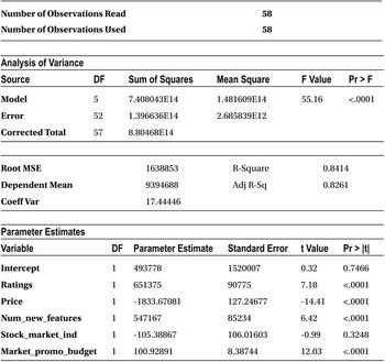
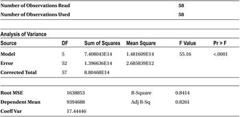
Table 10-4 gives the output of this code. In the ANOVA table, you can see the F-value and P-value of the F-test.
Table 10-4. Output of PROC REG on Mobiles Data Set
From the Analysis of Variance table, you can see that the F-value is 55.16, and the P-value of the F-test is less than 0.0001, which is way below the magic number of 5 percent. So, you can reject the null hypothesis. Now it’s safe to say that the model is meaningful for any further analysis. Generally, when R-squared is high, you see that the model is significant. In some cases where there are too many junk or insignificant variables in the model, R-squared and F-test behave differently. Please refer to the “R-squared and Adjusted R-Square (Adj R-sq)” section later in this chapter.
F-test: Additional Example
Let’s look at the simple regression example, price versus sales regression line.
proc reg data= mobiles;
model sales=price;
run;
Table 10-5 shows the result of the previous code.
Table 10-5. Output of PROC REG on Mobiles Data Set (model sales=price)
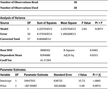
The F-value is 2.84, and the P-value of the F-test is 9.73 percent (0.0973). Since the P-value is greater than 5 percent, you don’t have enough evidence to reject H0, and you need to accept that the model is insignificant. In such a case, there is no point in looking further at the R-squared value. How much variance in y is explained by the model.
The T-test, T-value, and P-value of T-test
The T-test in regression is used to test the impact of individual variables. As discussed earlier, the F-test is used to determine the overall significance of a model. For example, in a regression model with ten independent variables, all may not be significant. Even if some insignificant independent variables are removed, there will not be any substantial effect on the predicting power of the model. The explanatory power of the model will largely remain the same after removal of less impacting variables. In mathematical terms, the beta coefficients of insignificant independent variables can be considered as zero.
For example, take the model for predicting smartphone sales. Do you need to keep all the independent variables? Are all relevant or significant? What if a junk variable such as the number of movie tickets sold is also included in the model? This model with a junk variable included might pass the F-test because there is at least one variable in the model that is significant. Consider the following questions, which are faced by every analyst while working on regression models:
- How do you identify the variables that have no impact on the model outcome (the dependent variable)?
- How do you test the impact of each individual variable?
- How do you test the effect of dropping or adding a variable in the model?
- Is there any way you can filter all the insignificant variables and have only significant variables in the model?
A T-test on regression coefficients will answer all these questions.
The null hypothesis on the T-test on regression coefficients is as follows:
H0:
 , which is equivalent to saying that coefficient of the independent variable (xi) is equal to zero. It also means that the variable xi has no impact on dependent variable y, and you can drop it from the model. The statistical inferences would be that the R-squared value will not get affected by dropping xi, and there will be no corresponding change in y for in every unit change in xi.
H1:
 , which would mean that the variable xi has some significant impact on the dependent variable and dropping xi would badly effect your model. In statistical terms, the R-squared value will drop significantly by dropping xi, and there will be some corresponding change in y for every unit change in xi.
To test the previous hypothesis, you calculate the T-statistic, which is also known as the T-value. Based on the T-value, you accept or reject the null hypothesis. In other words, the T-value will finally decide whether you should consider or reject a variable in the model. The T-value is calculated using the beta coefficients against a normal distribution of beta coefficients with a zero mean. Like the F-test, here also you look at the P-value of the T-statistic to determine the impact of a variable on the model.
If the P-value of a T-test is less than 5 percent, then you reject null hypothesis H0. In other words, you reject the premise that the variable has no impact. That means the variable is useful, and it has some explanatory power or some minimal impact on the dependent variable. If the T-test has a P-value greater than 5 percent, then you don’t have sufficient evidence to reject H0, which may force you to accept the null hypothesis (and eventually remove that variable from the model). In simple terms, look at the P-value of the T-test; if it is greater than 5 percent, then your variable is in trouble and you may need drop it. If the P-value less than 5 percent, there is no reason to worry, and you can keep the variable in your model and proceed with further analysis.
Example: T-test to Determine the Impact of Independent Variables
In the smartphone sales example, if you want to determine the impact of each independent variable, you need to look at the P-value of the T-tests in the output. Because there are five independent variables, you will have five T-tests, five T-values, and five P-values for the T-tests. There will be one more P-value for intercept in the Parameters Estimate table, which is not given much importance.
There will be no change in the following code:
/* Multiple Regression line for Smartphone sales example*/

proc reg data= mobiles;
model sales= Ratings Price Num_new_features Stock_market_ind Market_promo_budget;
run;
Table 10-6 shows the output of this code.
Table 10-6. Output of PROC REG on Mobiles Data Set
The P-value of the T-test for all the independent variables except stock market are less than 5 percent. So, the null hypothesis will be rejected in the case of Ratings, Price, Num_new_features, and Market_promo_budget. It would mean that these variables have some impact on the dependent variable, in other words, smartphone sales, whereas stock market (Stock_market_ind) has no impact on sales of smartphones. You come to this conclusion by looking at the P-value of the T-test for the stock market variable, which is greater than 5 percent (0.05), and there is not enough evidence to reject H0. You may have to accept the hypothesis that the stock market indicator has no impact on the sales.
Verifying the Impact of the Individual Variable
In the previous example, you made two inferences based on T-tests.
- The stock market has no impact on the dependent variable (y, the smartphone sales). This variable is not explaining a significant portion of variations in y.
- The rest of the independent variables, Ratings, Price, Num_new_features, and Market_promo_budget, have significant impact on the sale of smartphones.
Let’s validate the first inference. You will drop the variable Stock_market_ind and rebuild the model. The R-squared value including this variable is 84.14 percent. Let’s see the R-squared value of the model excluding this variable.
/* Multiple Regression model without Stock_market_ind */

proc reg data= mobiles;
model sales= Ratings Price Num_new_features  Market_promo_budget;
run;
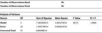
Table 10-7 shows the output of this code.
Table 10-7. Output of PROC REG on Mobiles Data Set (Excluding stock_market_ind Variable)
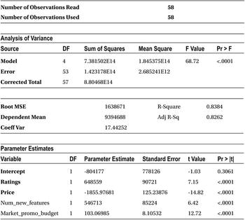
The important metric to note here is the R-squared value, which is 83.84 percent. The change in R-square is insignificant (earlier 84.14 percent). You can now safely conclude that the stock market index has nothing to do with smartphone sales.
Let’s validate the second inference. You will drop the variable ratings and rebuild the model. The R-squared value including this variable is 83.84 percent. Let’s see the R-squared value excluding this variable.
/* Multiple Regression model without Ratings */
proc reg data= mobiles;
model sales= Price Num_new_features  Market_promo_budget  ;
run;
Table 10-8 shows the output for this code.
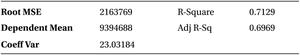
Table 10-8. Output of PROC REG on mobiles Variable with Price, Num_new_features, and Market_promo_budget

The new R-square value is 68.25 percent, which has dropped significantly from 83.84 percent. This forces you to accept the fact that the ratings variable has significant impact on the model outcome. By removing this variable, you are losing a considerable amount of explanatory power of the model.
In fact, the R-square value will change significantly for all the other high-impact variables. In the following text, we have repeated the regression model with different combinations of independent variables. Tables 10-9 through 10-11 list the R-square for these models.
The following is the SAS code to build a regression model with a dependent variable sales and independent variables as ratings, num_new_features, and market_promo_budget.
proc reg data= mobiles;
model sales= Ratings Num_new_features Market_promo_budget;
run;
Table 10-9 lists the output of this code.
Table 10-9. R-square with Ratings, Num_new_features, and Market_promo_budget
![]()
The following is the SAS code to build a regression model with a dependent variable sales and independent variables as ratings, price, and market_promo_budget.
proc reg data= mobiles;
model sales= Ratings Price Market_promo_budget ;
run;
Table 10-10 lists the output of this code.
Table 10-10. R-square with Ratings, price and Market_promo_budget
The following is the SAS code to build a regression model with a dependent variable sales and independent variables as ratings, price, and num_new_features.
proc reg data= mobiles;
model sales= Ratings Price Num_new_features ;
run;
Table 10-11 lists the output of this code.
Table 10-11. R-square with Ratings, Price and Num_new_features
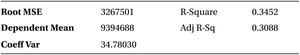
Figure 10-5 shows the change in the R-squared value when the variable is in the model and the R-squared value when the variable is dropped from the model.
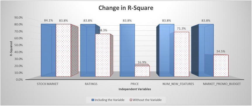
Figure 10-5. Change in R-square values
Looking at the previous results, you should have no hesitation in believing the T-test results about the impact of independent variables.
The R-squared and Adjusted R-square (Adj R-sq)
In the regression output you might have already observed the adjusted R-squared value near the R-squared. It is known as adjusted R-square. To understand the importance of the adjusted R-square, let’s look at an example.
Import the sample regression data (sample_regression.csv); it is a simple simulated data set with some independent variables along with a dependent variable. Build three models on this data and note the R-square and adjusted R-square values for the three models. The following are the specifications for building the models:
- First model with independent variables: x1, x2, x3
- Second model with independent variables: x1, x2..x6
- Third model with all the variables: x1, x2…x8
/* Importing Sample Regression Data Set*/

PROC IMPORT OUT= WORK.sample_regression
            DATAFILE= "C:UsersVENKATGoogle DriveTrainingBooksContent
Multiple and Logistic Regressionsample_regression.csv"
            DBMS=CSV REPLACE;
     GETNAMES=YES;
     DATAROW=2;
RUN;
Model 1: Y vs. x1,x2,x3
/* Regression on Sample Regression Data set*/
proc reg data=sample_regression;
model y=x1 x2 x3;
run;
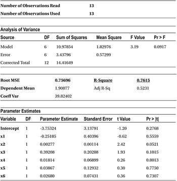
Table 10-12 shows the result of this code. Please take note of the R-squared and adjusted R-squared values.
Table 10-12. Output of PROC REG on simple_regression Data Set (model y=x1 x2 x3)
Model 2: Y vs. x1,x2,…x6
proc reg data=sample_regression;
model y=x1 x2 x3 x4 x5 x6;
run;
Table 10-13 shows the result of this code. Please take note of the R-squared and adjusted R-squared values.
Table 10-13. Output of PROC REG on simple_regression Data Set (model y=x1 x2 x3 x4 x5 x6)
Model 3: Y vs. x1,x2,…x8
proc reg data=sample_regression;
model y=x1 x2 x3  x4 x5 x6 x7 x8;
run;
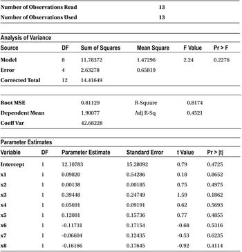
Table 10-14 shows the result of the previous code. Please take note of the R-squared and adjusted R-squared values.
Table 10-14. Output of PROC REG on simple_regression Data Set (model y=x1 x2 x3 x4 x5 x6 x7 x8)
Analysis on Three Models
Figure 10-6 shows the R-squared and adjusted R-squared results from the previous three models.
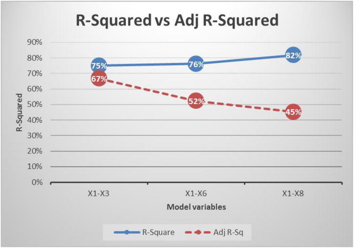
Figure 10-6. R-squared and adjusted R-squared values for the three models
When you build the model with just the three variables x1, x2, and x3, the R-square and adjusted R-squared values are very close. As you keep adding more and more variables, the gap between the R-square and adjusted R-squared values widens. Though R-square is a good measure to explain the variation in y, there is a small challenge in its formula.
Limitations of R-Squared
The following are the limitations:
- The R-squared will either increase or remain the same when adding a new independent variable to the model. It will never decrease unless you remove a variable.
- Once R-square reaches a maximum point with a set of variables, then it will never come down by adding another independent variable to the set. There may be some minute upward improvements in the R-square value. Even if the newly added variable has no impact on the model outcome, there can be some marginal improvements in the R-squared value.
- Here is an easy way to understand this feature: R-squared is the total amount of variation explained by the list of independent variables in the model. If you add any new junk independent variable, a variable that has no impact or relation with dependent variable, the R-square still might increase slightly, but it will never decrease.
It is favorable (to an analyst) that R-squared increases when you have a decent or high-impact on dependent variable. But what happens to the R-squared value if a junk or trivial variable is added to the model? R-squared will not show any significant increase when you add junk variables. But still there will be a small positive increment. Let’s assume that there is just a 0.5 percent increment in the R-squared value for the addition of every such junk variable. If you add 50 such junk variables, you might see a whopping 25 percent growth in the value of R-square. That is not an insignificant increase by any measure. It happens particularly when there is fewer observations (records or rows) in the data. Adding a new variable quickly impacts, and an increase the R-squared value is seen.
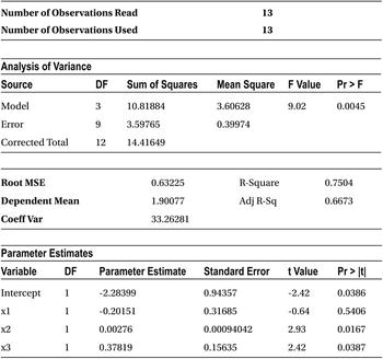
In the previous example, let’s analyze the output of the final model, namely, model 3 as given in Table 10-15.
Table 10-15. Output of model 3
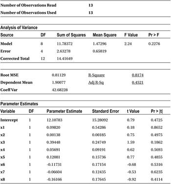
Here are some observations from the previous result:
- There are just 13 records in the data. It’s a small sample, so there are few observations to analyze.
- Most of the variables have absolutely no impact on the dependent variable as per the T-test. The P-value for all the variables in the T-test is greater than 5 percent.
- Even the F-test tells you that the overall model is insignificant because the P-value of the F-test is 22.76 percent, which is greater than the magic number of 0.5 percent.
- Still the R-square is 81.74 percent.
This is the point we want to make here. The R-square value from model 1 to model 2 jumped from 75 percent to 76 percent, and then finally for model 3 it went on to become 82 percent. The R-squared will further increase if you add some more variables to model 3. So, you need to be careful while inferring anything based on R-squared values.
A combination of fewer observations and many independent variables is a highly vulnerable situation in regression analysis. It is like cheating ourselves by adding junk independent variables and feeling thrilled about increments in R-square. But on the ground, the whole model itself may be junk.
This behavior of R-squared establishes the need for a different measure that can give a reliable measure of the predicting power of any given model. Adjusted R-squared does exactly that.
Adjusted R-squared
Adjusted R-squared is derived from R-squared only. What are the expectations from this new measure? The adjusted R-squared is expected to be as follows:
- A measure that will give an idea about the explained variations in a model.
- A measure that will penalize the model when a junk variable is added.
- A measure that will take into account both the number of observations and the number of independent variables in a model.
- A measure that will increase only when a significant or impactful independent variable is added. It will decrease for the addition of any junk or trivial variable to the model.
Adjusted R-squared meets all these expectations. The following is the formula for adjusted R-squared:
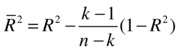
where
- R2 is the usual R-squared.
- n is the number of records.
- k is the number of independent variables.
Adjusted R-squared adds a penalty to R-squared for every new junk variable added. It shows an increase only for the addition of meaningful or high-impact variables to the model.
Let’s revisit the R-squared and adjusted R-squared comparison chart; see Figure 10-7.
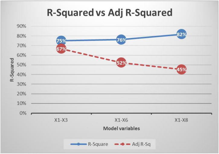
Figure 10-7. R-squared and adjusted R-squared for the three models
Looking at the adjusted R-squared values, you can conclude that only three variables (x1 to x3) are sufficient for the model to realize its maximum potential. As you go on adding new variables (x4 to x8), adjusted R-squared is showing a decrease. It indicates that all the incoming variables from x4 until x8 are junk variables, and they have no impact on y.
Adjusted R-square: Additional Example
For the smartphone sales example, you will first observe the full model results; in other words, the regression model will use all five independent variables.
/* Smartphone sales R-Squared and Adj-R Squared*/
proc reg data= mobiles;
model sales= Ratings Price Num_new_features Stock_market_ind Market_promo_budget;
run;
Table 10-16 gives the result of this code.
Table 10-16. Output of PROC REG on Mobiles Data Set
The R-squared and adjusted R-squared values are almost near but not the same, shown here:
|
R-square |
0.8414 |
|
Adj R-Sq |
0.8261 |
There is a small difference between the values if R-square and adjusted R-sq. Why is this? In earlier sections, using T-tests, you found that the stock market has no significant impact on the sales of smartphones. Maybe this is the variable that is triggering that small difference between the R-squared and adjusted R-squared values. You will remove the stock market indicator variable and rebuild the model. You will observe that the R-squared and adjusted R-squared values are getting closer.
proc reg data= mobiles;
model sales= Ratings Price Num_new_features Market_promo_budget;
run;
Table 10-17 shows the output for this code.
Table 10-17. Output of PROC REG on Mobiles Data Set

The R-squared and adjusted R-squared got slightly closer. But there is still a difference without any insignificant variable in the model. This is because of the fewer records. If there are large records and no junk variables, the R-square and adjusted R-squared values can be the same.
When Can You Be Dependent Upon Only R-squared?
You can use R-squared in these cases:
- It is safe to consider adjusted R-squared all the time. In fact, it’s recommended.
- If the sample size is adequately large compared to the number of independent variables and if all the independent variables have significant impact, then you may consider R-squared value as the goodness of fit measure. Otherwise, adjusted R-squared is the right measure.
Multiple Regression: Additional Example
The SAT is a standardized test widely used for college admissions in the United States. Let’s build a regression model for predicting the SAT scores based on students’ high-school marks. Students may need a high proficiency in subjects such as mathematics, general knowledge (GK), science, and general aptitude at the high-school level in order to get high scores in SAT. After collecting some historical data for close to 100 students, say you try to build a model that will predict the SAT score based on the scores obtained in the high-school exams.
The following is the code to import the data:
/* importing SAT exam Data*/
PROC IMPORT OUT= WORK.sat_score
            DATAFILE= "C:UsersVENKATGoogle DriveTrainingBooksContent
Multiple and Logistic RegressionSAT_Exam.csv"
            DBMS=CSV REPLACE;
     GETNAMES=YES;
     DATAROW=2;
RUN;
The following is the code for printing the snapshot of the data file. The data file contains some historical data on the actual marks obtained in the high-school exams.
proc print data= sat_score(obs=10) ;
run;
In Table 10-18, you can see that there are four independent variables called general knowledge (GK), aptitude (apt), mathematics (math), and science, along with one dependent variable, SAT. The idea is to fit a model using these four independent variables to predict the SAT score.
/* Predicting SAT score using rest of the Variables*/

proc reg data=sat_score;
model SAT=General_knowledge Aptitude Mathematics Science;
run;
Table 10-18. Four independent variables to predict the SAT score

Table 10-19 is the output for this code.
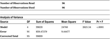
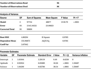
Table 10-19. Output of PROC REG on sat_score Data Set

Here are observations from the previous output:
- As expected, the analyst would be curious to look at the R-squared value to see whether the model is a good fit. In other words, how much of the variation in the target variable (the SAT score) is explained by independent variables (marks in four high-school subjects)? However, you should first look at the F-value or the P-value of the F-test, which tells whether the model is a significant one. If the P-value is greater than 5 percent, then there is no need to go further down through the output. In that case, you stop at the F-test and say the model is insignificant. If the P-value of the F-test is less than 5 percent, then there is at least one variable that is significant, which means the model may have some impact. In this model, the P-value of the F-test is less than 5 percent; in fact, it is less than 0.0001, as is evident from the output (Analysis of Variance table). The model looks significant, and you can take a further look at other measures like R-squared and T-test.
- The R-squared and adjusted R-squared values are almost same at around 99 percent, which is a really good sign. So, the overall model is explaining almost 99 percent of variations in Y. In other words, if you know a student’s marks in aptitude, GK, science, and mathematics, you can precisely predict her SAT score.
- Now let’s take a look at the impact of each variable (Table 10-20).
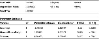
Table 10-20. The Parameter Estimate Table from the Output of PROC REG on sat_score Data Set

From the Parameters Estimates table (Table 10-20), you observe that mathematics and aptitude do not have any significant effect on the dependent variable (SAT score). You will remove these two variables and rebuild the model with just two variables: science and general knowledge (GK).
/* Predicting SAT score using two variables only*/

proc reg data=sat_score;
model SAT=General_knowledge Science ;
run;
Table 10-21 shows the output for this code.
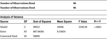
From the previous output, you can observe the following:
- The p-value of the F-test is less than 0.0001, which is much less than the required magic number of 5 percent, so the model is significant.
- The R-squared and adjusted R-squared values are close to 100 percent.
- The P-values of the T-tests show that all the variables have significant impact on y. For both GK and science, the P-values are less than 0.0001, which again is much superior to the required condition of a P-value less than 5 percent.
- You can go ahead and use the model for predictions.
Some Surprising Results from the Previous Model
In the same SAT score example, when you consult a domain expert, you come to know that math and aptitude are two important “should have” skills to get good scores on the SAT. The domain expert tells you from her experience that the SAT scores of students are dependent on the marks obtained by them in math and aptitude at the high-school level. But the model is telling the opposite story.
Let’s build a model using mathematics and aptitude scores alone. If they are really not impacting the SAT scores, then you should see all negative results in F-tests, R-squared values, and T-tests.
proc reg data=sat_score;
model SAT=Mathematics Aptitude ;
run;
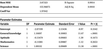
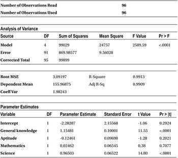
Table 10-22 shows the output of this code.
Table 10-22. Output of PROC REG on sat_score Data Set
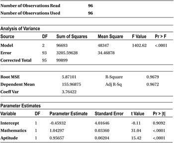
Here are some observations from the previous output:
- F-test: The P-values are less than 5 percent, so the model is significant. It’s strange and surprising.
- R-squared and adjusted R-squared: This is 96 percent, which utterly surprising and contrary to what was expected.
- T-tests : The P-values of both the variable are less than 5 percent; this is again a shocking result.
- Earlier mathematics and aptitude had negative coefficients; now they have positive coefficients with the same historical data file. The results this time are very much in agreement with what the domain expert suggested.
A model, on the same historical data with all four subjects (xi), showed that mathematics and aptitude scores have no impact at all. Another model, on the same data with two subjects, is showing completely contrary results. Why are mathematics and aptitude insignificant in the presence of science and GK?
- Why did removing science and GK from the model affect the impact of mathematics and aptitude? In generic terms, why did removing some variables affect the impact of other variables, without affecting overall model predictive power?
- Are these independent variables related in some manner? Is there any interrelation between these independent variables that is causing these changes in T-test results?
Let’s forget about the dependent variable for some time and observe the intercorrelation between the independent variables. Here is the code:
proc corr data=sat_score;
var General_knowledge Aptitude Mathematics Science ;
run;
Table 10-23 shows the output of this code.
Table 10-23. Output of PROC REG on sat_score Data Set
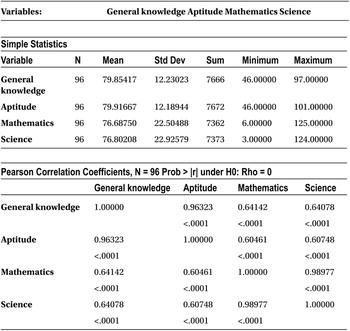
We’ve formatted the same correlation table for better readability (Table 10-24).
Table 10-24. Correlation Table for Sat Score Example
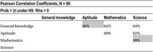
The correlation between GK and aptitude is 96 percent; the correlation between mathematics and science is 99 percent. This should be the reason why the mathematics and aptitude variables were insignificant in the presence of science and GK, and they had significant impact without them. This phenomenon of interdependency is called multicollinearity. It is not just the pairwise correlation between two variables, but an independent variable can depend on any number of independent variables. This multicollinearity can lead to many false inferences and absurd results. An analyst needs to take this multicollinearity challenge seriously.
Multicollinearity is a phenomenon where you see a high interdependency between the independent variables. When you refer to multicollinearity, you talk about independent variables (xi) only. The dependent variable y is nowhere in the picture. Multicollinearity is not just about the relation between a pair of variables and a given independent variable set. Sometimes multiple independent variables together might be related to another independent variable. So, any significant relation or association in the independent variables set is considered as multicollinearity (Figure 10-8).
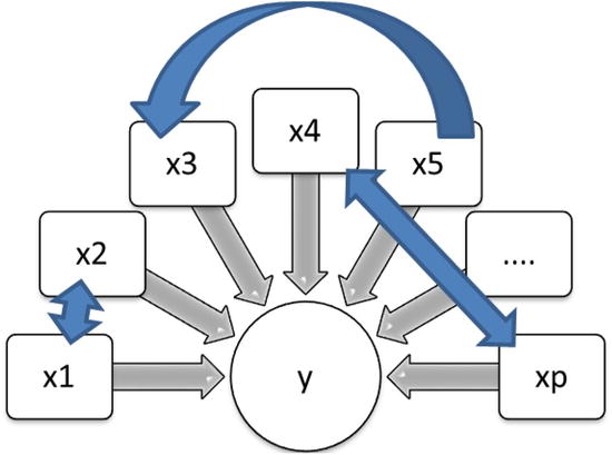
Figure 10-8. Multicollinearity
Why Is Multicollinearity a Problem? The Effects of Multicollinearity
In the SAT score example discussed earlier, you saw some indications of what multicollinearity can lead to. Here is a list of challenges that multicollinearity can create:
- Let’s discuss the significance of beta coefficients. In a model like y = 3X1 + 6.5X2 - 0.3X3, what does each coefficient indicate? A beta coefficient is nothing but the increment in dependent variable (y) for every unit change in independent variable, keeping all other independent variables constant. In this regression line, x1 has a coefficient of 3; it indicates that y increases by 3 units for every unit change in x1, keeping x2 and x3 constant. But what if there is multicollinearity? What if x2 is dependent upon x1? A regression coefficient has no meaning in this case. The increment in y for every unit change in x1 is 3, keeping x2 and x3 constant. But this condition of keeping x2 and x3 constant will not hold good if x2 is dependent upon x1. In other words, x2 also changes because of the change in x1. This is a multicollinearity effect.
- In the presence of multicollinearity, the coefficients that are coming out of the regression model are not stable. Sometimes the coefficients and even their signs might be misleading. In the case of multicollinearity, the regression coefficients will have a high standard deviation, which means that even for small changes in the data (observations), the changes in the regression coefficients may be abnormally high. Sometimes with a small change in the data, the coefficient signs might change. In other words, if a variable shows a positive impact with one set of data, with a small change in the data, it might show a negative impact.
- With multicollinearity in place, the T-test results are not trustworthy. You can’t really look at T-test’s P-value and make a decision about the impact of any independent variable.
Let’s again take a look at the SAT exam’s regression model.
/* Predicting SAT score using rest of the four variables. General_knowledge, Aptitude, Mathematics, and Science */

proc reg data=sat_score;
model SAT=General_knowledge Aptitude Mathematics Science;
run;
Table 10-25 shows the output for this code.
In this example, here are the false implications because of multicollinearity:
- You can see that mathematics and aptitude are negatively impacting the SAT score. In other words, if the mathematics score increases, then the SAT score decreases. If the aptitude score increases, then the SAT score decreases.
- Mathematics and aptitude have no impact on SAT score.
- General knowledge has a higher impact than aptitude and mathematics.
Let’s make a small change in the data file and observe the corresponding changes in the beta coefficients. Ideally, if the model is stable, there should be minimal changes in all the coefficient estimates. As shown in Table 10-26, you will change the mathematics score from 102 to 60 in the second row.
Table 10-26. Highlighting the Changes in Mathematics Score in sat_score Data Set
![]()
Table 10-27 shows the results of the new model built with this update in the data file.
Table 10-27. Output of PROC REG on sat_score data set with Math Score Changed
The output now has one important and big change. The beta coefficient of mathematics is positive now. With just one value changed from 102 to 60, the coefficient of mathematics turned upside down. This is what we are trying to emphasize as the adverse effect of multicollinearity.
The following is another way of looking at the high standard deviation or coefficient changes in the presence of multicollinearity:
- Let’s build a new model: Y vs. X1, X2, and X3. Here you have a significant multicollinearity relationship between X2 and X3.
- Assume that X3 has a near to straight line relationship with X2. And X3 is nearly equal to two times X2, which can be denoted by X3 ~ 2X2.
- Let’s assume that the final model equation is Y=X1+20X2-2X2. Please note, there is a negative coefficient for X2 (-2).
Now you will try to establish that in the presence of multicollinearity, the coefficients are so unstable that they might even change their signs without affecting predictive power of the overall model (overall R-square will remain the same).
- The model Y=X1+20X2-2X3
- The multicollinearity X3 ~ 2X2
- The model rewritten Y=X1+ 14X2+6X2-2X3
- The model rewritten Y ~ X1+14X2+ 3X3-2X3 (put X2=X3/2)
- The model rewritten Y ~ X1+14X2+ X3
So, with multicollinearity, the original model Y=X1+20X2-2X3 finally ends to Y ~ X1+14 X2+ X3. The coefficient of X3 has turned from negative to positive. Similarly, you can play around this model and make the coefficient almost anything. This is exactly what we are talking about—the instability in regression coefficients and high standard deviation in beta coefficient estimates.
In simple terms, if there is an existence of multicollinearity in a model, the regression coefficients can’t be trusted for any meaningful analysis.
The multicollinearity challenge raises three questions:
- What are the causes of multicollinearity?
- How do you identify the existence of multicollinearity in my model?
- Once multicollinearity is identified, what is the way out? How can its effect be minimized?
What Are the Causes of Multicollinearity?
Multicollinearity as such is not a result of any mistake in your analysis. If there is some interdependency in the independent variables, there is nothing wrong from the analyst side. An analyst needs to be aware of this, and it should be taken care of when building an accurate regression model. The following are some causes of multicollinearity:
- The way data was collected might result in multicollinearity. Are you choosing all independent, nonassociated variables while collecting the data?
- Too many variables explaining the same piece of information might be one of the causes of multicollinearity. For example, the variables such as average yearly income, average tax paid, and net yearly savings might be related to each other in most cases. All these variables are explaining a person’s financial position.
- Specifying the model variables inaccurately might be one more cause. For example, a variable X and its multiple are present in a model. Another example is when X and a polynomial term related to X are present in a model.
- Having too many independent variables can also result into multicollinearity. Having too many independent variables and fewer records has never been a good idea in regression modeling. Sometimes options are not available, and you need to proceed. In such cases, an analyst needs to deal with the multicollinearity challenge.
Identification of Multicollinearity
As you have seen, multicollinearity is a serious challenge for an analyst. It is caused by some known or unknown reasons (or an unknown relation between variables sometimes). Now every time you will be in a position to explain why two variables are related. Analysts need to be alert and identify multicollinearity in the model building phase; otherwise, it may lead to irrational inferences.
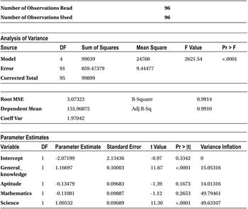
Multicollinearity can be identified using correlation techniques. By finding the correlation, you can see the strength of association between two variables. If there is a high correlation, it means that the model has multicollinearity. The existence of correlation is sufficient to say that there is multicollinearity. But the correlation may not be always high even if there is multicollinearity in the model. A simple correlation is not enough to identify all types of multicollinearity. Correlation is just a pairwise association measure, so you will not be able to quantify the association if one independent variable is associated loosely to two or more independent variables. (If the pairwise association is loose, multicollinearity will not be evident in correlation, and you need a different measure.) All the associated variables together can strongly explain the variation in that particular independent variable. Let’s take an example where x2, x3, and x5 are related to x4 (Figure 10-9).
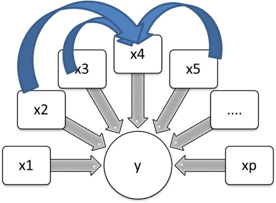
Figure 10-9. Multicollinearity: x2, x3, and x5 are related to x4
Forget about Y for some time and see whether the three variables x2, x3, and x5 are really impacting variations in x4. You need a measure that will quantify the relation between multiple variables. How do you get an idea of the combined impact of several independent variables on a dependent variable? In this context, x2, X3, X5 are independent variables, and x4 is the dependent variable. Refer to Figure 10-10.

Figure 10-10. X4 is taken as a dependent variable, and x2, x3, and x5 are related to x4
We build a regression model using these independent variables and observe the value of R-squared. If the R-square value is high for the model x4 versus x2, x3, and x5, then the variable x4 can be explained by the other three. This will indicate interdependency or multicollinearity.
To detect the multicollinearity within a set of independent variables, you first need to choose the different subsets in the group. Regression lines are built for these subsets, and the R-square value is checked for each line.
Here is the overall model:
- y vs. y1 , y2, y3………….yp
- Here are models for detecting multicollinearity:
- x1 vs. x2, x3…….xp
 R-squared value (R21)
 - x2 vs. x1, x3…….xp R-squared value (R22)
- ………………………………………………………
- xp vs. x1, x2, x3…….xp-1 R-squared value (R2p)
- Finally, note the R21, R22 …………R2p values to detect the multicollinearity.
If the R-square value is high, then it is an indication of multicollinearity. An R-squared value of more than 80 percent is considered as a good indicator for the existence of multicollinearity.
Variance Inflation Factor (VIF)
VIF is a measure that is specifically defined to measure the multicollinearity.
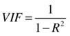
So, the higher the R-square value, the higher the VIF value will be. In fact, VIF will magnify the R-squared value. If the R-squared value is 80 percent, then the VIF value will be 5. Refer to Table 10-28.
Table 10-28. R-squared and VIF Values
![]()
Note: Do not confuse this R-Squared with overall model’s R-Squared value. This R-square is calculated by building the models between the independent variables.
If the VIF value for a variable is greater than 5, it indicates strong multicollinearity and that variable can be termed as redundant. This is because 80 percent or more of the variation in that variable is explained by rest of the independent variables. So, it is mandatory to see the VIF values while building a multiple regression line.
Let’s take the SAT score example again and calculate VIF values to check whether there is any multicollinearity. In this model, you already know about it, but you will use VIF values to confirm the same. PROC REG in SAS has a VIF option that will calculate VIF values for each variable. You do not need to worry about finding each VIF value separately for different combinations of the independent variables.
The following is the code for displaying VIF values in the output; you need to add the keyword VIF in the model statement:
proc reg data=sat_score;
model SAT=General_knowledge Aptitude Mathematics Science/VIF;
run;
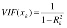
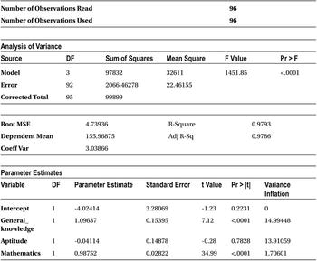
Table 10-29 shows the output of this code.
Table 10-29. Output of PROC REG on sat_score
Though the output looks the same as any other multiple regression output, there is a new column added in the Parameter Estimates table: Variance Inflation. This is just the VIF value. So, you see that column and check whether there are any variables with VIF more than 5.
In this output, all the variables have VIF values greater than 5, but it doesn’t imply that all four variables are interrelated. Generally, VIF values appear in pairs. If you remove one variable from the pair, the other one is automatically corrected. For example, let’s remove science from the model and check the multicollinearity again.
proc reg data=sat_score;
model SAT=General_knowledge Aptitude Mathematics /VIF ;
run;
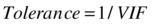
Please refer to Table 10-30 for the output.
Table 10-30. Output of PROC REG on sat_score
You can see a massive change in the VIF value for mathematics. In the same way, if you remove mathematics, you will see the science variable VIF changed to 1.7.
The following facts are worth noting in case of multicollinearity:
- VIF is a measure that helps in detecting multicollinearity. The correlation matrix can also help sometimes, but VIF takes care of all the variables.
- The F-test and T-test behaving in a contrasting manner is also an indication of multicollinearity. A high F-statistic and R-squared value will make you believe that the overall model is a good fit. The T-tests, on other hand, may show that most of the variables are not having any impact on y. This situation is caused by multicollinearity.
- The wrong signs for the coefficients or counterintuitive estimates for the known variables is another sign of multicollinearity.
- You can make a small change in the sample or the input data and observe the changes in the regression coefficients. If these changes are abnormally high, then it is an indication of multicollinearity.
- The condition number is another way of identifying high standard deviations in the beta coefficients. Instead of directly finding the associations between the independent variables, the condition number looks at the expected variance in the beta coefficient. If the condition number is high, it is an indicator of multicollinearity. As a rule of thumb, if the condition number is more than 30, it is a sign of multicollinearity. A more detailed discussion on this topic is beyond the scope of this book.
- Tolerance is another measure, which is used as an indicator of the multicollinearity. Tolerance is nothing but the inverse of VIF. So, nothing really is new in it.
 .
.
Up to now, we have discussed the challenges that occur because of multicollinearity. We have also discussed ways to detect it. In the following section, we will discuss how to treat multicollinearity while building a regression model.
Redemption of Multicollinearity (Treating Multicollinearity)
Multicollinearity is seen most of the times as a redundancy. This means that all of the variables involving multicollinearity are not required in the model. Other truly independent variables in the model are sufficient to explain the variations in the final dependent variable. Consider building a model for Y using X1, X2, X3, X4, and X5. If X2, X3, and X5 are explaining more than 80 percent of variations in X4, then there is no need to keep X4 in the model. You can very well drop X4 from the model specification and rebuild an accurate enough model for Y using X1, X2, X3, and X5 alone.
Dropping Troublesome Variables
In most of the cases you go ahead and drop the troublesome variables from the independent variable list. But you need to be careful. You can’t simply drop all the variables having a VIF value greater than 5. As discussed earlier, the VIF values come in pairs. If you drop a variable, the other one is adjusted automatically.
Let’s look at the VIF values for the SAT exam data (Table 10-31).
Table 10-31. VIF Values for SAT Exam Data
VIF values for all the variables are greater than 5. But as expected, they all are in pairs (with two values close to each other). You take the highest pair and drop a variable from there. Here mathematics has a slightly higher VIF, and you can drop it. Here both math and science have almost the same VIF values, so you keep the most important variable (in the context of the business problem). Otherwise, you can go ahead and drop the variable with the highest VIF.
Here is the model-building code after dropping mathematics:
proc reg data=sat_score;
model SAT=General_knowledge Aptitude Science/VIF;
run;
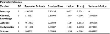
Please refer to Table 10-32 for the output.
Table 10-32. VIF Values for SAT Exam Data After Dropping Mathematics
The variable science looks fine now. VIF is still high for GK and aptitude. Let’s drop GK and rebuild the model. Here is the code:
proc reg data=sat_score;
model SAT= Aptitude  Science/VIF;
run;
Please refer to Table 10-33 for the output.
Table 10-33. Output of PROC REG on sat_score with Only Aptitude and Science
Everything seem to be perfect with this model. There is no multicollinearity, so you can trust these coefficients. The coefficient signs are also intuitively correct (from the business knowledge angle) for both the variables.
Other Ways of Treating Multicollinearity
Though dropping troublesome variables is the most widely used method, there are a few other ways of dealing the multicollinearity.
- You can use principal components instead of variables. Principal components are linear combinations of variables, which will be explaining maximum variance in the data. If some variables are intercorrelated, you can use noncorrelated linear combination of variables instead of directly using the variables.
- On having a good understanding of the causes of multicollinearity, an analyst can reduce it by collecting more data and a better unbiased sample.
- If prediction is the only motto and the relationship with Y and xi is not of interest, the same model with interdependent independent variables may be used. If the model with correlated Xi still has a high R-squared value, it may be good enough for prediction purposes. The challenges comes only when the interest is in analyzing a one-to-one relationship between independent and dependent variables.
- Ridge regression is another way to treat the multicollinearity. The main philosophy behind the ridge regression is that it’s better to get a biased estimated of betas with less standard deviation instead of unbiased beta estimates with a high standard deviation. So, ridge regression does some tweaking to the optimization matrix while finding the least square estimates of regression coefficients. The details are beyond the scope of this book.
- Data transformation may yield good results sometimes.
How to Analyze the Output: Linear Regression Final Check List
In this chapter you learned several measures and several challenges that need careful treatment. This check list will help you; you can remember it with the acronym FRAVT, which stands for F-test, R-squared, adjusted R-squared, VIF, and T-tests.
Double-Check for the Assumptions of Linear Regression
You have to make sure that all the regression assumptions are religiously followed by the data (observations) before attempting to build a model. Generally this process takes a lot of time. Many analysts tend to ignore this step and take it for granted that all the regression assumptions are followed. Generally, a scatterplot is drawn between the Xi and Y variables to verify the linearity assumption. Here you get almost 90 percent of an idea about the existence of outliers, nonlinearity, heteroscedasicity, and so on. If all regression assumptions are followed, only then can you move on to the next check point, the F-test. Most of the time analysts come to know about possible assumption violations when they are right in the middle of analysis and something goes wrong.
The first measure to look at in this order is the F-test. It gives you an idea about the overall significance of a model. If an F-test shows that the model is not significant, there is no need to go any further in the model-building process. You can simply stop the model building and look for other impacting variables to predict y. You can search for more data or do some more research to check whether there are any vital errors at any stage in the overall model-building process. If F-test is passed, in other words, the model is established as significant, you can move on to the next check point of the R-squared value.
R-squared
The R-squared value comes after conforming the fact that the model is significant. R-squared will tell you how significant the model is. A higher R-squared value (greater than 80 percent) indicates that model is explaining the maximum variation in the dependent variable.
Because R-squared has some downsides while using multiple regression methodology, you also have to look at the adjusted R-squared value and make sure that there are no junk variables or the model is over specified with too many independent variables.
The next step is to make sure that there is no multicollinearity within the independent variables. You can check it using the VIF values of each variable. If multicollinearity is detected, then proper treatment needs to be given to the independent variables in order to prepare an independent set of predictor variables.
The final item in the list is the T-test. The T-test results tell you about the most impacting variables. You can safely drop all the nonimportant variables and keep only the most impacting ones. Sometimes a number of model iterations are required to identify and keep few most-impacting variables. This may involve compromising a little bit on the R-squared value to reduce number of variables.
Analyzing the Regression Output: Final Check List Example
Let’s, once again, observe the output of smartphone sales data. You can assume that the analyst has already validated the data against all the assumptions of linear regression. The following is the code, SAS output (Table 10-34), and final checklist steps:
proc reg data= mobiles;
model sales= Ratings Price Num_new_features Stock_market_ind Market_promo_budget/vif;
run;
Please refer to Table 10-34 for the output.
Here is the check list:
- Assumptions of regression: You already tested that the data doesn’t violate any of the linear regression assumptions.
- F-test: This looks good; the model is significant.
- R-squared: More than 80 percent of variance in y is explained by xi. Hence, the model is a good fit.
- Adjusted R-squared: This is slightly less than R-squared, indicating some junk variable is in the data. Are there any insignificant variables? Yes, the stock market indicator is insignificant; you can drop it and rebuild the model.
proc reg data= mobiles;
model sales= Ratings Price Num_new_features Market_promo_budget/vif;
run;
Please refer to Table 10-35 for the output.
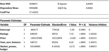
Here is the check list:
- Assumptions of regression: It is already given that the data doesn’t violate regression assumptions.
- F-test: This looks good; the model is significant.
- R-squared: More than 80 percent of variance of explanation is a good fit.
- Adjusted R-squared: This is almost close to R-squared, so no junk values are in the model.
- The VIF values are all within the limits; there are no multicollinearity threats.
- All variables pass the T-test and show that all of them have significant impact on sales.
The model is ready to be used for smartphone sales perditions. Given the values of Ratings, Price, Num_new_features, and Market_promo_budget, the accuracy will be more than 80 percent. The following is the final model equation for predictions:

Conclusion
In this chapter, you started with multiple linear regressions to tackle the predictions where more than one independent variable is used. You also learned the goodness of fit measures for multiple regression. The multiple regression has several independent variables, and their interdependency may lead to absurd results. You learned how to handle the multicollinearity issue. Finally, you saw a checklist to be used while analyzing the multiple regression output. Several concepts were simplified and dealt with at a basic level. You may need to refer to dedicated text books on regression to get some in-depth theory behind these concepts.
We talked about linear regression. Obviously you can’t expect all the relations in this world to be linear. What if you come across a nonlinear relationship between dependent (y) and independent (xi) variables? How do you build a nonlinear regression line? What are the changes in the assumptions? What are the goodness of fit measures? What are the other challenges involved in the process? Nonlinear regression is the topic of the next chapter. Stay tuned!