
Chapter 7. Primitive Assembly and Rasterization
This chapter describes the types of primitives and geometric objects that are supported by OpenGL ES, and explains how to draw them. It then describes the primitive assembly stage, which occurs after the vertices of a primitive are processed by the vertex shader. In the primitive assembly stage, clipping, perspective divide, and viewport transformation operations are performed. These operations are discussed in detail. The chapter concludes with a description of the rasterization stage. Rasterization is the process that converts primitives into a set of two-dimensional fragments, which are processed by the fragment shader. These two-dimensional fragments represent pixels that may be drawn on the screen.
Refer to Chapter 8, “Vertex Shaders,” for a detailed description of vertex shaders. Chapter 9, “Texturing,” and Chapter 10, “Fragment Shaders,” describe processing that is applied to fragments generated by the rasterization stage.
Primitives
A primitive is a geometric object that can be drawn using the glDrawArrays, glDrawElements, glDrawRangeElements, glDrawArraysInstanced, and glDrawElementsInstanced commands in OpenGL ES. The primitive is described by a set of vertices that indicate the vertex position. Other information, such as color, texture coordinates, and geometric normal can also be associated with each vertex as generic attributes.
The following primitives can be drawn in OpenGL ES 3.0:
• Triangles
• Lines
• Point sprites
Triangles
Triangles represent the most common method used to describe a geometry object rendered by a 3D application. The triangle primitives supported by OpenGL ES are GL_TRIANGLES, GL_TRIANGLE_STRIP, and GL_TRIANGLE_FAN. Figure 7-1 shows examples of supported triangle primitive types.
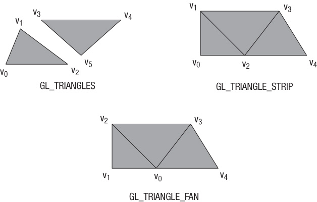
GL_TRIANGLES draws a series of separate triangles. In Figure 7-1, two triangles given by vertices (v0, v1, v2) and (v3, v4, v5) are drawn. A total of n/3 triangles are drawn, where n is the number of indices specified as count in glDraw*** APIs mentioned previously.
GL_TRIANGLE_STRIP draws a series of connected triangles. In the example shown in Figure 7-1, three triangles are drawn given by (v0, v1, v2), (v2, v1, v3) (note the order), and (v2, v3, v4). A total of (n – 2) triangles are drawn, where n is the number of indices specified as count in glDraw*** APIs.
GL_TRIANGLE_FAN also draws a series of connected triangles. In the example shown in Figure 7-1, the triangles drawn are (v0, v1, v2), (v0, v2, v3), and (v0, v3, v4). A total of (n – 2) triangles are drawn, where n is the number of indices specified as count in glDraw*** APIs.
Lines
The line primitives supported by OpenGL ES are GL_LINES, GL_LINE_STRIP, and GL_LINE_LOOP. Figure 7-2 shows examples of supported line primitive types.
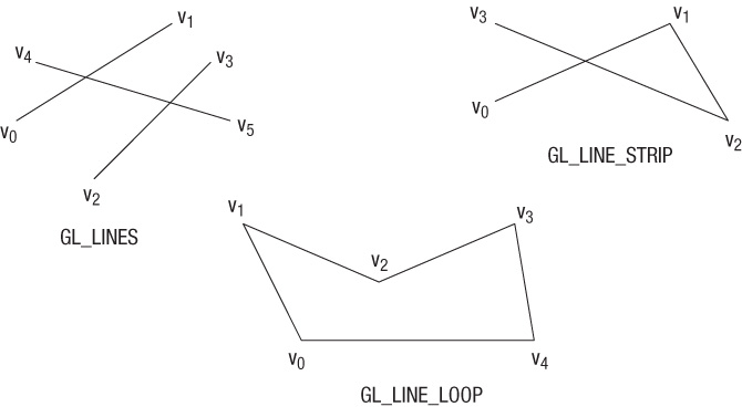
GL_LINES draws a series of unconnected line segments. In the example shown in Figure 7-2, three individual lines are drawn given by (v0, v1), (v2, v3), and (v4, v5). A total of n/2 segments are drawn, where n is the number of indices specified as count in glDraw*** APIs.
GL_LINE_STRIP draws a series of connected line segments. In the example shown in Figure 7-2, three line segments are drawn given by (v0, v1), (vl, v2), and (v2, v3). A total of (n – 1) line segments are drawn, where n is the number of indices specified as count in glDraw*** APIs.
GL_LINE_LOOP works similar to GL_LINE_STRIP, except that a final line segment is drawn from vn–1 to v0. In the example shown in Figure 7-2, the line segments drawn are (v0, v1), (v1, v2), (v2, v3), (v3, v4), and (v4, v0). A total of n line segments are drawn, where n is the number of indices specified as count in glDraw*** APIs.
The width of a line can be specified using the glLineWidth API call.
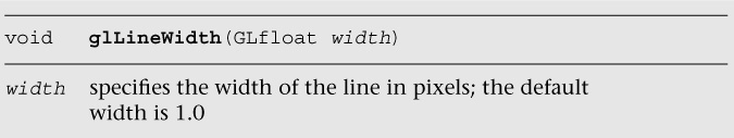
The width specified by glLineWidth will be clamped to the line width range supported by the OpenGL ES 3.0 implementation. In addition, the width specified will be remembered by OpenGL until updated by the application. The supported line width range can be queried using the following command. There is no requirement for lines with widths greater than 1 to be supported.
GLfloat lineWidthRange[2];
glGetFloatv ( GL_ALIASED_LINE_WIDTH_RANGE, lineWidthRange );
Point Sprites
The point sprite primitive supported by OpenGL ES is GL_POINTS. A point sprite is drawn for each vertex specified. Point sprites are typically used for rendering particle effects efficiently by drawing them as points instead of quads. A point sprite is a screen-aligned quad specified as a position and a radius. The position describes the center of the square, and the radius is then used to calculate the four coordinates of the quad that describes the point sprite.
gl_PointSize is the built-in variable that can be used to output the point radius (or point size) in the vertex shader. It is important that a vertex shader associated with the point primitive output gl_PointSize; otherwise, the value of the point size is considered undefined and will most likely result in drawing errors. The gl_PointSize value output by a vertex shader will be clamped to the aliased point size range supported by the OpenGL ES 3.0 implementation. This range can be queried using the following command:
GLfloat pointSizeRange[2];
glGetFloatv ( GL_ALIASED_POINT_SIZE_RANGE, pointSizeRange );
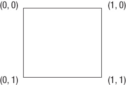
By default, OpenGL ES 3.0 describes the window origin (0, 0) to be the (left, bottom) region. However, for point sprites, the point coordinate origin is (left, top).
gl_PointCoord is a built-in variable available only inside a fragment shader when the primitive being rendered is a point sprite. It is declared as a vec2 variable using the mediump precision qualifier. The values assigned to gl_PointCoord go from 0.0 to 1.0 as we move from left to right or from top to bottom, as illustrated in Figure 7-3.
The following fragment shader code illustrates how gl_PointCoord can be used as a texture coordinate to draw a textured point sprite:
#version 300 es
precision mediump float;
uniform sampler2D s_texSprite;
layout(location = 0) out vec4 outColor;
void main()
{
outColor = texture(s_texSprite, gl_PointCoord);
}
Drawing Primitives
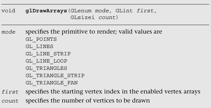
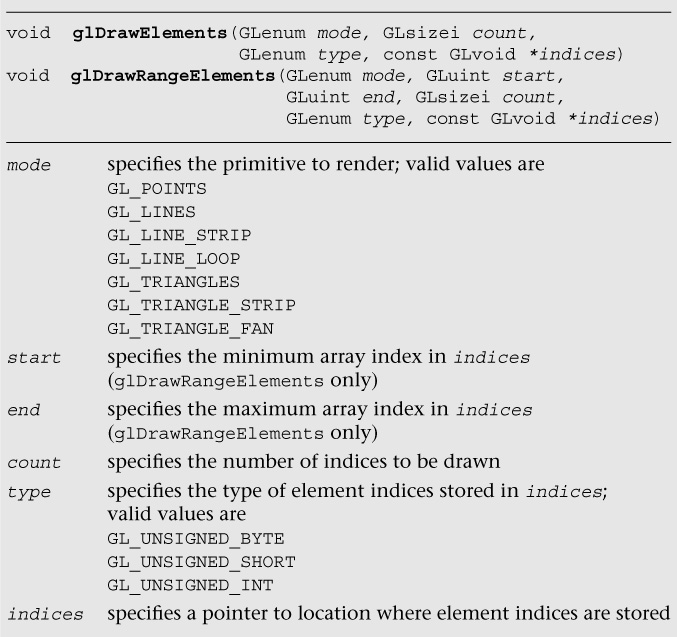
There are five API calls in OpenGL ES to draw primitives: glDrawArrays, glDrawElements, glDrawRangeElements, glDrawArraysInstanced, and glDrawElementsInstanced. We will describe the first three regular non-instanced draw call APIs in this section and the remaining two instanced draw call APIs in the next section.
glDrawArrays draws primitives specified by mode using vertices given by element index first to first + count – 1. A call to glDrawArrays (GL_TRIANGLES, 0, 6) will draw two triangles: a triangle given by element indices (0, 1, 2) and another triangle given by element indices (3, 4, 5). Similarly, a call to glDrawArrays(GL_TRIANGLE_STRIP, 0, 5) will draw three triangles: a triangle given by element indices (0, 1, 2), the second triangle given by element indices (2, 1, 3), and the final triangle given by element indices (2, 3, 4).
glDrawArrays is great if you have a primitive described by a sequence of element indices and if vertices of geometry are not shared. However, typical objects used by games or other 3D applications are made up of multiple triangle meshes where element indices may not necessarily be in sequence and vertices will typically be shared between triangles of a mesh.
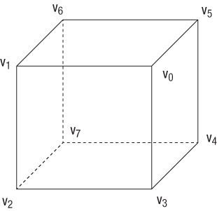
Consider the cube shown in Figure 7-4. If we were to draw this using glDrawArrays, the code would be as follows:
#define VERTEX_POS_INDX 0
#define NUM_FACES 6
GLfloat vertices[] = { ... }; // (x, y, z) per vertex
glEnableVertexAttribArray ( VERTEX_POS_INDX );
glVertexAttribPointer ( VERTEX_POS_INDX, 3, GL_FLOAT,
GL_FALSE, 0, vertices );
for (int i=0; i<NUM_FACES; i++)
{
glDrawArrays ( GL_TRIANGLE_FAN, i*4, 4 );
}
Or
glDrawArrays ( GL_TRIANGLES, 0, 36 );
To draw this cube with glDrawArrays, we would call glDrawArrays for each face of the cube. Vertices that are shared would need to be replicated, which means that instead of having 8 vertices, we would now need to allocate 24 vertices (if we draw each face as a GL_TRIANGLE_FAN) or 36 vertices (if we use GL_TRIANGLES). This is not an efficient approach.
This is how the same cube would be drawn using glDrawElements:
#define VERTEX_POS_INDX 0
GLfloat vertices[] = { ... };// (x, y, z) per vertex
GLubyte indices[36] = {0, 1, 2, 0, 2, 3,
0, 3, 4, 0, 4, 5,
0, 5, 6, 0, 6, 1,
7, 1, 6, 7, 2, 1,
7, 5, 4, 7, 6, 5,
7, 3, 2, 7, 4, 3 };
glEnableVertexAttribArray ( VERTEX_POS_INDX );
glVertexAttribPointer ( VERTEX_POS_INDX, 3, GL_FLOAT,
GL_FALSE, 0, vertices );
glDrawElements ( GL_TRIANGLES,
sizeof(indices)/sizeof(GLubyte),
GL_UNSIGNED_BYTE, indices );
Even though we are drawing triangles with glDrawElements and a triangle fan with glDrawArrays and glDrawElements, our application will run faster than glDrawArrays on a GPU for many reasons. For example, the size of vertex attribute data will be smaller with glDrawElements as vertices are reused (we will discuss the GPU post-transform vertex cache in a later section). This also leads to a smaller memory footprint and memory bandwidth requirement.
Primitive Restart
Using primitive restart, you can render multiple disconnected primitives (such as triangle fans or strips) using a single draw call. This is beneficial to reduce the overhead of the draw API calls. A less elegant alternative to using primitive restart is generating degenerate triangles (with some caveats), which we will discuss in a later section.
Using primitive restart, you can restart a primitive for indexed draw calls (such as glDrawElements, glDrawElementsInstanced, or glDrawRangeElements) by inserting a special index into the indices list. The special index is the largest possible index for the type of the indices (such as 255 or 65535 when the index type is GL_UNSIGNED_BYTE or GL_UNSIGNED_SHORT, respectively).
For example, suppose two triangle strips have element indices of (0, 1, 2, 3) and (8, 9, 10, 11), respectively. The combined element index list if we were to draw both strips using one call to glDrawElements* with primitive restart would be (0, 1, 2, 3, 255, 8, 9, 10, 11) if the index type is GL_UNSIGNED_BYTE.
You can enable and disable primitive restart as follows:
glEnable ( GL_PRIMITIVE_RESTART_FIXED_INDEX );
// Draw primitives
...
glDisable ( GL_PRIMITIVE_RESTART_FIXED_INDEX );
Provoking Vertex
Without qualifiers, output values of the vertex shader are linearly interpolated across the primitive. However, with the use of flat shading (described in the Interpolation Qualifiers section in Chapter 5), no interpolation occurs. Because no interpolation occurs, only one of the vertex values can be used in the fragment shader. For a given primitive instance, the provoking vertex determines which of the vertices output from the vertex shader are used, as only one can be used. Table 7-1 shows the rule for the provoking vertex selection.
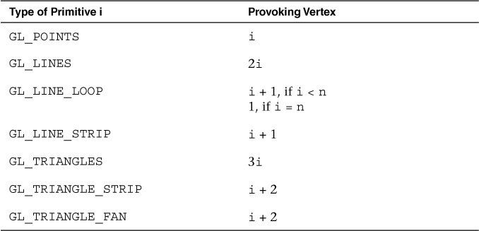
Table 7-1 Provoking Vertex Selection for the ith Primitive Instance Where Vertices Are Numbered from 1 to n, and n Is the Number of Vertices Drawn
Geometry Instancing
Geometry instancing allows for efficiently rendering an object multiple times with different attributes (such as a different transformation matrix, color, or size) using a single API call. This feature is useful in rendering large quantities of similar objects, such as in crowd rendering. Geometry instancing reduces the overhead of CPU processing to send many API calls to the OpenGL ES engine. To render using an instanced draw call, use the following commands:
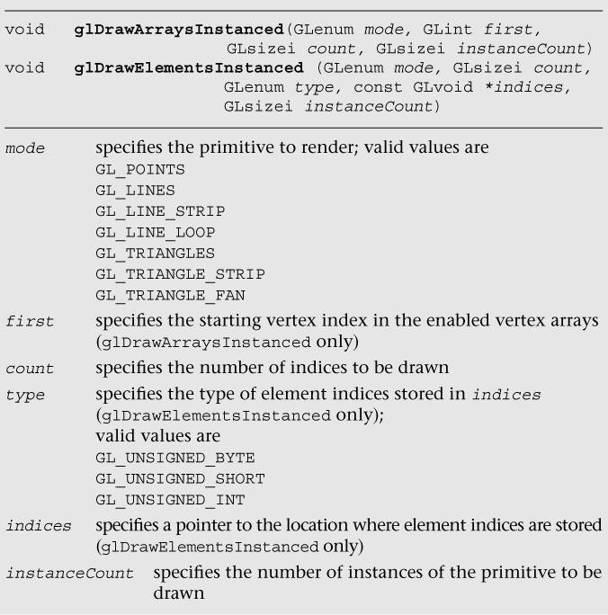
Two methods may be used to access per-instance data. The first method is to instruct OpenGL ES to read vertex attributes once or multiple times per instance using the following command:
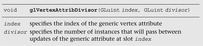
By default, if glVertexAttribDivisor is not specified or is specified with divisor equal to 0 for the vertex attributes, then the vertex attributes will be read once per vertex. If divisor equals 1, then the vertex attributes will be read once per primitive instance.
The second method is to use the built-in input variable gl_InstanceID as an index to a buffer in the vertex shader to access the per-instance data. gl_InstanceID will hold the index of the current primitive instance when the previously mentioned geometry instancing API calls are used. When a non-instanced draw call is used, gl_InstanceID will return 0.
The next two code fragments illustrate how to draw many geometry (i.e., cubes) using a single instanced draw call where each cube instance will be colored uniquely. Note that the complete source code is available in Chapter_7/Instancing example.
First, we create a color buffer to store many color data to be used later for the instanced draw call (one color per instance).
// Random color for each instance
{
GLubyte colors[NUM_INSTANCES][4];
int instance;
srandom ( 0 );
for ( instance = 0; instance < NUM_INSTANCES; instance++ )
{
colors[instance][0] = random() % 255;
colors[instance][1] = random() % 255;
colors[instance][2] = random() % 255;
colors[instance][3] = 0;
}
glGenBuffers ( 1, &userData->colorVBO );
glBindBuffer ( GL_ARRAY_BUFFER, userData->colorVBO );
glBufferData ( GL_ARRAY_BUFFER, NUM_INSTANCES * 4, colors,
GL_STATIC_DRAW );
}
After the color buffer has been created and filled, we can bind the color buffer as one of the vertex attributes for the geometry. Then, we specify the vertex attribute divisor as 1 so that the color will be read per primitive instance. Finally, the cubes are drawn with a single instanced draw call.
// Load the instance color buffer glBindBuffer ( GL_ARRAY_BUFFER, userData->colorVBO );
glVertexAttribPointer ( COLOR_LOC, 4, GL_UNSIGNED_BYTE,
GL_TRUE, 4 * sizeof ( GLubyte ),
( const void * ) NULL );
glEnableVertexAttribArray ( COLOR_LOC );
// Set one color per instance
glVertexAttribDivisor ( COLOR_LOC, 1 );
// code skipped ...
// Bind the index buffer
glBindBuffer ( GL_ELEMENT_ARRAY_BUFFER, userData->indicesIBO );
// Draw the cubes
glDrawElementsInstanced ( GL_TRIANGLES, userData->numIndices,
GL_UNSIGNED_INT,
(const void *) NULL, NUM_INSTANCES );
Performance Tips
Applications should make sure that glDrawElements and glDrawElementsInstanced are called with as large a primitive size as possible. This is very easy to do if we are drawing GL_TRIANGLES. However, if we have meshes of triangle strips or fans, instead of making individual calls to glDrawElements* for each triangle strip mesh, these meshes could be connected together by using primitive restart (see the earlier section discussing this feature).
If you cannot use the primitive restart mechanism to connect meshes together (to maintain compatibility with an older OpenGL ES version), you can add element indices that result in degenerate triangles at the expense of using more indices and some caveats that we will discuss here. A degenerate triangle is a triangle where two or more vertices of the triangle are coincident. GPUs can detect and reject degenerate triangles very easily, so this is a good performance enhancement that allows us to queue a big primitive to be rendered by the GPU.
The number of element indices (or degenerate triangles) we need to add to connect distinct meshes will depend on whether each mesh is a triangle fan or a triangle strip and the number of indices defined in each strip. The number of indices in a mesh that is a triangle strip matters, as we need to preserve the winding order as we go from one triangle to the next triangle of the strip across the distinct meshes that are being connected.
When connecting separate triangle strips, we need to check the order of the last triangle and the first triangle of the two strips being connected. As seen in Figure 7-5, the ordering of vertices that describe even-numbered triangles of a triangle strip differs from the ordering of vertices that describe odd-numbered triangles of the same strip.
Two cases need to be handled:
• The odd-numbered triangle of the first triangle strip is being connected to the first (and therefore even-numbered) triangle of the second triangle strip.
• The even-numbered triangle of the first triangle strip is being connected to the first (and therefore even-numbered) triangle of the second triangle strip.
Figure 7-5 shows two separate triangle strips that represent these two cases, where the strips need to be connected to allow us to draw both of them using a single call to glDrawElements*.
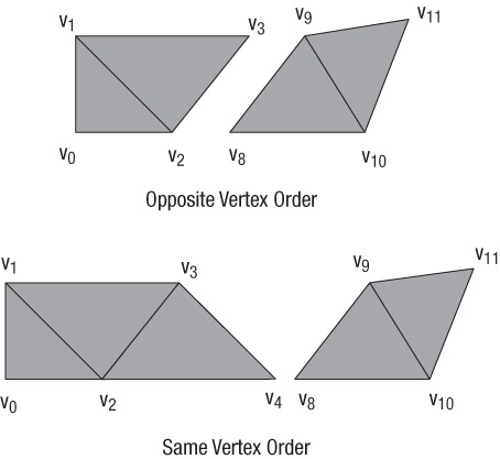
For the triangle strips in Figure 7-5 with opposite vertex order for the last and first triangles of the two strips being connected, the element indices for each triangle strip are (0, 1, 2, 3) and (8, 9, 10, 11), respectively. The combined element index list if we were to draw both strips using one call to glDrawElements* would be (0, 1, 2, 3, 3, 8, 8, 9, 10, 11). This new element index results in the following triangles drawn: (0, 1, 2), (2, 1, 3), (2, 3, 3), (3, 3, 8), (3, 8, 8), (8, 8, 9), (8, 9, 10), (10, 9, 11). The triangles in boldface type are the degenerate triangles. The element indices in boldface type represent the new indices added to the combined element index list.
For triangle strips in Figure 7-5 with the same vertex order for the last and first triangles of the two strips being connected, the element indices for each triangle strip are (0, 1, 2, 3, 4) and (8, 9, 10, 11), respectively. The combined element index list if we were to draw both strips using one call to glDrawElements would be (0, 1, 2, 3, 4, 4, 4, 8, 8, 9, 10, 11). This new element index results in the following triangles drawn: (0, 1, 2), (2, 1, 3), (2, 3, 4), (4, 3, 4), (4, 4, 4), (4, 4, 8), (4, 8, 8), (8, 8, 9), (8, 9, 10), (10, 9, 11). The triangles in boldface type are the degenerate triangles. The element indices in boldface type represent the new indices added to the combined element index list.
Note that the number of additional element indices required and the number of degenerate triangles generated vary depending on the number of vertices in the first strip. This is required to preserve the winding order of the next strip being connected.
It might also be worth investigating techniques that take the size of the post-transform vertex cache into consideration in determining how to arrange element indices of a primitive. Most GPUs implement a post-transform vertex cache. Before a vertex (given by its element index) is executed by the vertex shader, a check is performed to determine whether the vertex already exists in the post-transform cache. If the vertex exists in the post-transform cache, the vertex is not executed by the vertex shader. If it is not in the cache, the vertex will need to be executed by the vertex shader. Using the post-transform cache size to determine how element indices are created should help overall performance, as it will reduce the number of times a vertex that is reused gets executed by the vertex shader.
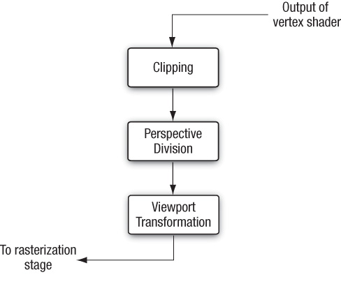
Primitive Assembly
Figure 7-6 shows the primitive assembly stage. Vertices that are supplied through glDraw*** are executed by the vertex shader. Each vertex transformed by the vertex shader includes the vertex position that describes the (x, y, z, w) value of the vertex. The primitive type and vertex indices determine the individual primitives that will be rendered. For each individual primitive (triangle, line, and point) and its corresponding vertices, the primitive assembly stage performs the operations shown in Figure 7-6.
Before we discuss how primitives are rasterized in OpenGL ES, we need to understand the various coordinate systems used within OpenGL ES 3.0. This is needed to get a good understanding of what happens to vertex coordinates as they go through the various stages of the OpenGL ES 3.0 pipeline.
Coordinate Systems
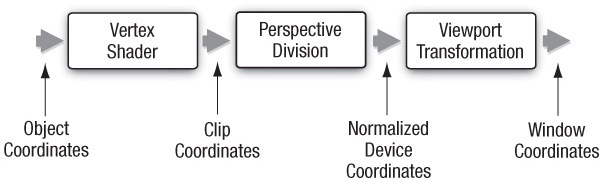
Figure 7-7 shows the coordinate systems as a vertex goes through the vertex shader and primitive assembly stages. Vertices are input to OpenGL ES in the object or local coordinate space. This is the coordinate space in which an object is most likely modeled and stored. After a vertex shader executes, the vertex position is considered to be in the clip coordinate space. The transformation of the vertex position from the local coordinate system (i.e., object coordinates) to clip coordinates is done by loading the appropriate matrices that perform this conversion in appropriate uniforms defined in the vertex shader. Chapter 8, “Vertex Shaders,” describes how to transform the vertex position from object to clip coordinates and how to load appropriate matrices in the vertex shader to perform this transformation.
Clipping
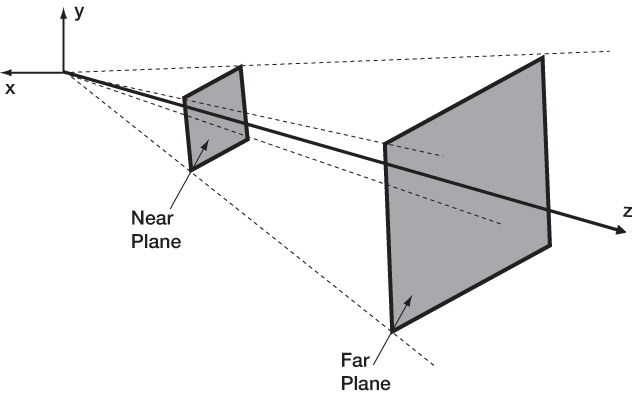
To avoid processing of primitives outside the viewable volume, primitives are clipped to the clip space. The vertex position after the vertex shader has been executed is in the clip coordinate space. The clip coordinate is a homogeneous coordinate given by (xc, yc, zc, wc). The vertex coordinates defined in clip space (xc, yc, zc, wc) get clipped against the viewing volume (also known as the clip volume).
The clip volume, as shown in Figure 7-8, is defined by six clipping planes, referred to as the near, and far clip planes, the left and right clip planes, and the top and bottom clip planes. In clip coordinates, the clip volume is given as follows:
-wc <= xc <= wc
-wc <= yc <= wc
-wc <= zc <= wc
The preceding six checks help determine the list of planes against which the primitive needs to be clipped.
The clipping stage will clip each primitive to the clip volume shown in Figure 7-8. By “primitive,” here we imply each triangle of a list of separate triangles drawn using GL_TRIANGLES, or a triangle of a triangle strip or a fan, or a line from a list of separate lines drawn using GL_LINES, or a line of a line strip or line loop, or a specific point in a list of point sprites. For each primitive type, the following operations are performed:
• Clipping triangles—If the triangle is completely inside the viewing volume, no clipping is performed. If the triangle is completely outside the viewing volume, the triangle is discarded. If the triangle lies partly inside the viewing volume, then the triangle is clipped against the appropriate planes. The clipping operation will generate new vertices that are clipped to the plane that are arranged as a triangle fan.
• Clipping lines—If the line is completely inside the viewing volume, then no clipping is performed. If the line is completely outside the viewing volume, the line is discarded. If the line lies partly inside the viewing volume, then the line is clipped and appropriate new vertices are generated.
• Clipping point sprites—The clipping stage will discard the point sprite if the point position lies outside the near or far clip plane or if the quad that represents the point sprite is outside the clip volume. Otherwise, it is passed unchanged and the point sprite will be scissored as it moves from inside the clip volume to the outside, or vice versa.
After the primitives have been clipped against the six clipping planes, the vertex coordinates undergo perspective division to become normalized device coordinates. A normalized device coordinate is in the range –1.0 to +1.0.
Note
The clipping operation (especially for lines and triangles) can be quite expensive to perform in hardware. A primitive must be clipped against six clip planes of the viewing volume, as shown in Figure 7-8. Primitives that are partly outside the near and far planes go through the clipping operations. However, primitives that are partially outside the x and y planes do not necessarily need to be clipped. By rendering into a viewport that is bigger than the dimensions of the viewport specified with glViewport, clipping in the x and y planes becomes a scissoring operation. Scissoring is implemented very efficiently by GPUs. This larger viewport region is called the guard-band region. Although OpenGL ES does not allow an application to specify a guard-band region, most—if not all—OpenGL ES implementations implement a guard-band.
Perspective Division
Perspective division takes the point given by clip coordinate (xc, yc, zc, wc) and projects it onto the screen or viewport. This projection is performed by dividing the (xc, yc, zc) coordinates with wc. After performing (xc/wc), (yc/wc), and (zc /wc), we get normalized device coordinates (xd, yd, zd). These are called normalized device coordinates, as they will be in the [–1.0 ... 1.0] range. These normalized (xd, yd) coordinates will then be converted to actual screen (or window) coordinates depending on the dimensions of the viewport. The normalized (zd) coordinate is converted to the screen z value using the near and far depth values specified by glDepthRangef. These conversions are performed in the viewport transformation phase.
Viewport Transformation
A viewport is a 2D rectangular window region in which all OpenGL ES rendering operations will ultimately be displayed. The viewport transformation can be set by using the following API call:
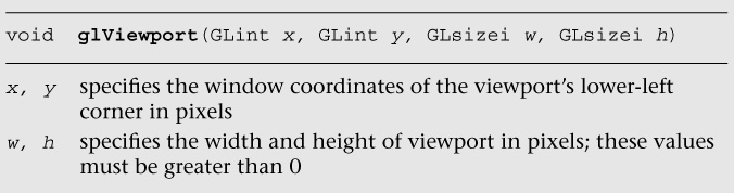
The conversion from normalized device coordinates (xd, yd, zd) to window coordinates (xw, yw, zw) is given by the following transformation:
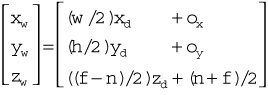
In the transformation ox = x + w/2 and oy = y + h/2, n and f represent the desired depth range.
The depth range values n and f can be set using the following API call:
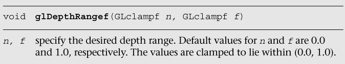
The values specified by glDepthRangef and glViewport are used to transform the vertex position from normalized device coordinates into window (screen) coordinates.
The initial (or default) viewport state is set to w = width and h = height of the window created by the application in which OpenGL ES is to do its rendering. This window is given by the EGLNativeWindowType win argument specified in eglCreateWindowSurface.
Rasterization
Figure 7-9 shows the rasterization pipeline. After the vertices have been transformed and primitives have been clipped, the rasterization pipelines take an individual primitive such as a triangle, a line segment, or a point sprite and generate appropriate fragments for this primitive. Each fragment is identified by its integer location (x, y) in screen space. A fragment represents a pixel location given by (x, y) in screen space and additional fragment data that will be processed by the fragment shader to produce a fragment color. These operations are described in detail in Chapter 9, “Texturing,” and Chapter 10, “Fragment Shaders.”
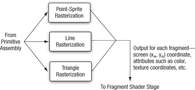
In this section, we discuss the various options that an application can use to control rasterization of triangles, strips, and fans.
Culling
Before triangles are rasterized, we need to determine whether they are front-facing (i.e., facing the viewer) or back-facing (i.e., facing away from the viewer). The culling operation discards triangles that face away from the viewer. To determine whether the triangle is front-facing or back-facing we first need to know the orientation of the triangle.
The orientation of a triangle specifies the winding order of a path that begins at the first vertex, goes through the second and third vertex, and ends back at the first vertex. Figure 7-10 shows two examples of triangles with clockwise and counterclockwise winding orders.
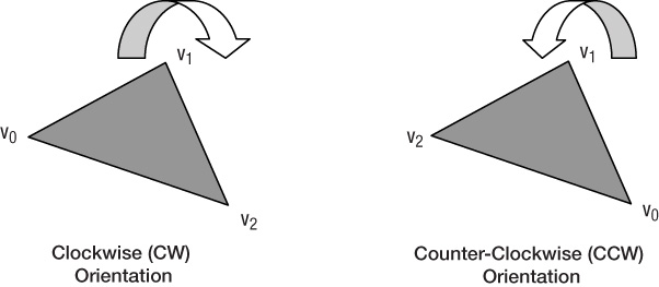
The orientation of a triangle is computed by calculating the signed area of the triangle in window coordinates. We now need to translate the sign of the computed triangle area into a clockwise (CW) or counterclockwise (CCW) orientation. This mapping from the sign of triangle area to a CW or CCW orientation is specified by the application using the following API call:
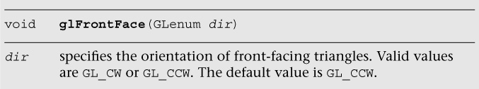
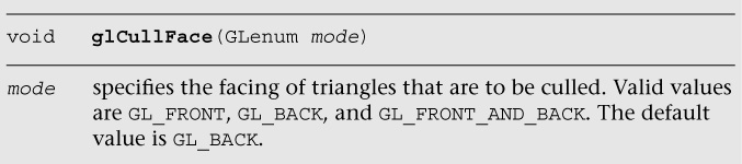
We have discussed how to calculate the orientation of a triangle. To determine whether the triangle needs to be culled, we need to know the facing of triangles that are to be culled. This is specified by the application using the following API call:
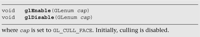
Last but not least, we need to know whether the culling operation should be performed. The culling operation will be performed if the GL_CULL_FACE state is enabled. The GL_CULL_FACE state can be enabled or disabled by the application using the following API calls:
To recap, to cull appropriate triangles, an OpenGL ES application must first enable culling using glEnable (GL_CULL_FACE), set the appropriate cull face using glCullFace, and set the orientation of front-facing triangles using glFrontFace.
Note
Culling should always be enabled to avoid the GPU wasting time rasterizing triangles that are not visible. Enabling culling should improve the overall performance of the OpenGL ES application.
Polygon Offset
Consider the case where we are drawing two polygons that overlap each other. You will most likely notice artifacts, as shown in Figure 7-11. These artifacts, called Z-fighting artifacts, occur because of limited precision of triangle rasterization, which can affect the precision of the depth values generated per fragment, resulting in artifacts. The limited precision of parameters used by triangle rasterization and generated depth values per fragment will get better and better but will never be completely resolved.
Figure 7-11 shows two coplanar polygons being drawn. The code to draw these two coplanar polygons without polygon offset is as follows:
glClear ( GL_COLOR_BUFFER_BIT | GL_DEPTH_BUFFER_BIT );
// load vertex shader
// set the appropriate transformation matrices
// set the vertex attribute state
// draw the SMALLER quad
glDrawArrays ( GL_TRIANGLE_FAN, 0, 4 );
// set the depth func to <= as polygons are coplanar glDepthFunc ( GL_LEQUAL );
// set the vertex attribute state
// draw the LARGER quad
glDrawArrays ( GL_TRIANGLE_FAN, 0, 4 );
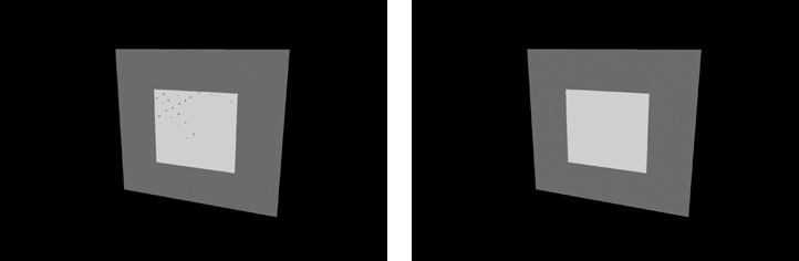
To avoid the artifacts shown in Figure 7-11, we need to add a delta to the computed depth value before the depth test is performed and before the depth value is written to the depth buffer. If the depth test passes, the original depth value—and not the original depth value + delta—will be stored in the depth buffer.
The polygon offset is set using the following API call:
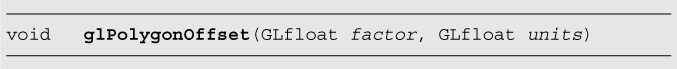
The depth offset is computed as follows:
depth offset = m * factor + r * units
In this equation, m is maximum depth slope of the triangle and is calculated as
m can also be calculated as max {|∂z/∂x|, |∂z/∂y|}.
The slope terms and are calculated by the OpenGL ES implementation during the triangle rasterization stage.
r is an implementation-defined constant and represents the smallest value that can produce a guaranteed difference in depth value.
Polygon offset can be enabled or disabled using glEnable(GL_POLYGON_OFFSET_FILL) and glDisable(GL_POLYGON_OFFSET_FILL), respectively.
With polygon offset enabled, the code for triangles rendered by Figure 7-11 is as follows:
const float polygonOffsetFactor = –l.Of;
const float polygonOffsetUnits = –2.Of;
glClear ( GL_COLOR_BUFFER_BIT | GL_DEPTH_BUFFER_BIT );
// load vertex shader
// set the appropriate transformation matrices
// set the vertex attribute state
// draw the SMALLER quad
glDrawArrays ( GL_TRIANGLE_FAN, 0, 4 );
// set the depth func to <= as polygons are coplanar
glDepthFunc ( GL_LEQUAL );
glEnable ( GL_POLYGON_OFFSET_FILL );
glPolygonOffset ( polygonOffsetFactor, polygonOffsetUnits );
// set the vertex attribute state
// draw the LARGER quad
glDrawArrays ( GL_TRIANGLE_FAN, 0, 4 );
Occlusion Queries
Occlusion queries use query objects to track any fragments or samples that pass the depth test. This approach can be used for a variety of techniques, such as visibility determination for a lens flare effect as well as optimization to avoid performing geometry processing on obscured objects whose bounding volume is obscured.
Occlusion queries can be started and ended using glBeginQuery and glEndQuery, respectively, with GL_ANY_SAMPLES_PASSED or GL_ANY_SAMPLES_PASSED_CONSERVATIVE target.
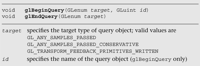
Using the GL_ANY_SAMPLES_PASSED target will return the precise boolean state indicating whether any samples passed the depth test. The GL_ANY_SAMPLES_PASSED_CONSERVATIVE target can offer better performance but a less precise answer. Using GL_ANY_SAMPLES_PASSED_CONSERVATIVE, some implementations may return GL_TRUE even if no sample passed the depth test.
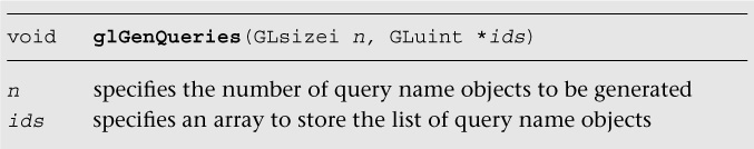
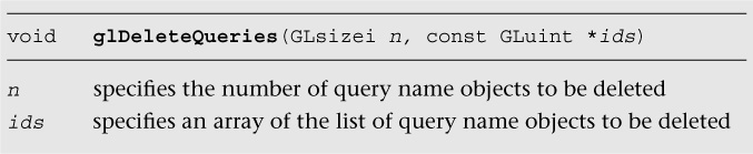
The id is created using glGenQueries and deleted using glDeleteQueries.
After you have specified the boundary of the query object using glBeginQuery and glEndQuery, you can use glGetQueryObjectuiv to retrieve the result of the query object.
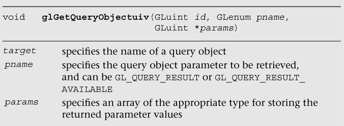
Note
For better performance, you should wait several frames before performing a glGetQueryObjectuiv call to wait for the result to be available in the GPU.
The following example shows how to set up an occlusion query object and query the result:
glBeginQuery ( GL_ANY_SAMPLES_PASSED, queryObject );
// draw primitives here
...
glEndQuery ( GL_ANY_SAMPLES_PASSED );
...
// after several frames have elapsed, query the number of
// samples that passed the depth test
glGetQueryObjectuiv( queryObject, GL_QUERY_RESULT,
&numSamples );
Summary
In this chapter, you learned the types of primitives supported by OpenGL ES, and saw how to draw them efficiently using regular non-instanced and instanced draw calls. We also discussed how coordinate transformations are performed on vertices. In addition, you learned about the rasterization stage, in which primitives are converted into fragments representing pixels that may be drawn on the screen. Now that you have learned how to draw primitives using vertex data, in the next chapter we describe how to write a vertex shader to process the vertices in a primitive.