15
Statistical Programming and Linear Regression
Data analysis and statistical processing are very import applications for modern programming languages. The subject area is vast. The Python ecosystem includes a number of add-on packages that provide sophisticated data exploration, analysis, and decision-making features.
We'll look at several topics, starting with some basic statistical calculations that we can do with Python's built-in libraries and data structures. This will lead to the question of correlation and how to create a regression model.
Statistical work also raises questions of randomness and the null hypothesis. It's essential to be sure that there really is a measurable statistical effect in a set of data. We can waste a lot of compute cycles analyzing insignificant noise if we're not careful.
Finally, we'll apply a common optimization technique. This can help to produce results quickly. A poorly designed algorithm applied to a very large set of data can be an unproductive waste of time.
In this chapter, we'll look at the following recipes:
- Using the built-in
statisticslibrary - Average of values in a counter
- Computing the coefficient of a correlation
- Computing regression parameters
- Computing an autocorrelation
- Confirming that the data is random – the
nullhypothesis - Locating outliers
- Analyzing many variables in one pass
We'll start by using the built-in statistics library. This provides useful results without requiring very sophisticated application software. It exemplifies the idea of the Python language having the batteries included – for some tasks, nothing more is needed.
Using the built-in statistics library
A great deal of exploratory data analysis (EDA) involves getting a summary of the data. There are several kinds of summary that might be interesting:
- Central Tendency: Values such as the mean, mode, and median can characterize the center of a set of data.
- Extrema: The minimum and maximum are as important as the central measures of a set of data.
- Variance: The variance and standard deviation are used to describe the dispersal of the data. A large variance means the data is widely distributed; a small variance means the data clusters tightly around the central value.
This recipe will show how to create basic descriptive statistics in Python.
Getting ready
We'll look at some simple data that can be used for statistical analysis. We've been given a file of raw data, called anscombe.json. It's a JSON document that has four series of (x,y) pairs.
We can read this data with the following command:
>>> from pathlib import Path
>>> import json
>>> from collections import OrderedDict
>>> source_path = Path('code/anscombe.json')
>>> data = json.loads(source_path.read_text())
We've defined the Path to the data file. We can then use the Path object to read the text from this file. This text is used by json.loads() to build a Python object from the JSON data.
We can examine the data like this:
>>> [item['series'] for item in data]
['I', 'II', 'III', 'IV']
>>> [len(item['data']) for item in data]
[11, 11, 11, 11]
The overall JSON document is a sequence of subdocuments with keys such as I and II. Each subdocument has two fields—series and data. The series key provides the name for the series. Within the data key, there is a list of observations that we want to characterize. Each observation has a pair of values.
    [
      {
        "series": "I",
        "data": [
          {
            "x": 10.0,
            "y": 8.04
          },
          {
            "x": 8.0,
            "y": 6.95
          },
          ...
        ]
      },
      ...
    ]
We can call this a List[Dict[str, Any]]. This summary, however, doesn't fully capture the structure of the dictionary. Each of the Series dictionaries has a number of very narrow constraints.
This is very close to the kinds of structures defined by the typing.TypedDict definition. We can almost use definitions like the following:
class Point(TypedDict):
    x: float
    y: float
class Series(TypedDict, total=False):
    series: str
    data: List[Point]
These definitions don't work as well as we'd like, however. When we define a dictionary this way, we're compelled to use literal keys when referencing the items in the dictionary. This isn't ideal for what we're doing, so we'll use a slightly weaker set of type definitions.
These type definitions capture the essence of the document with our raw data:
Point = Dict[str, float]
Series = Dict[str, Union[str, float, List[Point]]]
We've described each point as a mapping from a string, either x or y to a float value. We've defined the series as a mapping from a string, either series or data, to one of the following types; either str, float, or a List[Point] collection.
This doesn't capture the following additional details:
- The
serieskey maps to astring - The
datakey maps to aList[Point]collection
The annotation suggests that additional keys with float values may be added to this dictionary. The file as a whole can be described as a List[Series].
We'll look at the essential application of a few statistical functions to a number of closely related series of data. This core recipe serves as a basis for doing additional processing steps.
How to do it...
We'll start with a few steps to acquire the raw data. Once we've parsed the JSON document, we can define a collection of functions with a similar design pattern for gathering statistics.
- Reading the raw data is a matter of using the
json.loads()function to create aList[Series]structure that we can use for further processing. This was shown previously in the Getting ready section of this recipe. - We'll need a function to extract one of the variables from a
seriesstructure. This will return a generator that produces a sequence of values for a specific variable:def data_iter( series: Series, variable_name: str) -> Iterable[Any]: return ( item[variable_name] for item in cast(List[Point], series["data"]) ) - To compute summary statistics, we'll use a common template for a function. This has two comments to show where computations are done
(# Compute details here) and where results are displayed(# Display output here):def display_template(data: List[Series]) -> None: for series in data: for variable_name in 'x', 'y': samples = list( data_iter(series, variable_name)) # Compute details here. series_name = series['series'] print( f"{series_name:>3s} {variable_name}: " # Display output here. ) - To compute measures of central tendency, such as
meanandmedian, use thestatisticsmodule. Formode, we can use thestatisticsmodule or thecollections.Counterclass. This injectsmean(),median(), and construction of aCounter()into the template shown in the previous step:import statistics import collections def display_center(data: List[Series]) -> None: for series in data: for variable_name in 'x', 'y': samples = list( data_iter(series, variable_name)) mean = statistics.mean(samples) median = statistics.median(samples) mode = collections.Counter( samples ).most_common(1) series_name = series['series'] print( f"{series_name:>3s} {variable_name}: " f"mean={round(mean, 2)}, median={median}, " f"mode={mode}") - To compute the
variance, we'll need a similar design. There's a notable change in this design. The previous example computedmean,median, andmodeindependently. The computations of variance and standard deviation depend on computation of themean. This dependency, while minor in this case, can have performance consequences for a large collection of data:def display_variance(data: List[Series]) -> None: for series in data: for variable_name in 'x', 'y': samples = list( data_iter(series, variable_name)) mean = statistics.mean(samples) variance = statistics.variance(samples, mean) stdev = statistics.stdev(samples, mean) series_name = series['series'] print( f"{series_name:>3s} {variable_name}: " f"mean={mean:.2f}, var={variance:.2f}, " f"stdev={stdev:.2f}")
The display_center() function produces a display that looks like the following:
  I x: mean=9.0, median=9.0, mode=[(10.0, 1)]
  I y: mean=7.5, median=7.58, mode=[(8.04, 1)]
  II x: mean=9.0, median=9.0, mode=[(10.0, 1)]
  II y: mean=7.5, median=8.14, mode=[(9.14, 1)]
  III x: mean=9.0, median=9.0, mode=[(10.0, 1)]
  III y: mean=7.5, median=7.11, mode=[(7.46, 1)]
  IV x: mean=9.0, median=8.0, mode=[(8.0, 10)]
  IV y: mean=7.5, median=7.04, mode=[(6.58, 1)]
The essential design pattern means that we can use a number of different functions to compute different descriptions of the raw data. We'll look at ways to generalize this in the There's more… section of this recipe.
How it works...
A number of useful statistical functions are generally first-class parts of the Python standard library. We've looked in three places for useful functions:
- The
min()andmax()functions are built-in. - The
collectionsmodule has theCounterclass, which can create a frequency histogram. We can get themodefrom this. - The
statisticsmodule hasmean(),median(),mode(),variance(), andstdev(), providing a variety of statistical measures.
Note that data_iter() is a generator function. We can only use the results of this generator once. If we only want to compute a single statistical summary value, that will work nicely.
When we want to compute more than one value, we need to capture the result of the generator in a collection object. In these examples, we've used data_iter() to build a list object so that we can process it more than once.
There's more...
Our original data structure, data, is a sequence of mutable dictionaries. Each dictionary has two keys—series and data. We can update this dictionary with the statistical summaries. The resulting object can be saved for subsequent analysis or display.
Here's a starting point for this kind of processing:
import statistics
def set_mean(data: List[Series]) -> None:
    for series in data:
        for variable_name in "x", "y":
            result = f"mean_{variable_name}"
            samples = data_iter(series, variable_name)
            series[result] = statistics.mean(samples)
For each one of the data series, we've used the data_iter() function to extract the individual samples. We've applied the mean() function to those samples. The result is used to update the series object, using a string key made from the function name, mean, the _ character, and variable_name, showing which variable's mean was computed.
The output starts like this:
[{'data': [{'x': 10.0, 'y': 8.04},
           {'x': 8.0, 'y': 6.95},
           {'x': 13.0, 'y': 7.58},
           {'x': 9.0, 'y': 8.81},
           {'x': 11.0, 'y': 8.33},
           {'x': 14.0, 'y': 9.96},
           {'x': 6.0, 'y': 7.24},
           {'x': 4.0, 'y': 4.26},
           {'x': 12.0, 'y': 10.84},
           {'x': 7.0, 'y': 4.82},
           {'x': 5.0, 'y': 5.68}],
  'mean_x': 9.0,
  'mean_y': 7.500909090909091,
  'series': 'I'},
etc.
]
The other series are similar. Interestingly, mean values of all four series are nearly identical, even though the data is different.
If we want to extend this to include standard deviations or variance, we'd see that the outline of the processing doesn't change. The overall structure would have to be repeated using statistics.median(), min(), max(), and so on. Looking at changing the function from mean() to something else shows that there are two things that change in this boilerplate code:
- The
resultkey that is used to update theseriesdata - The function that's evaluated for the selected sequence of samples
The similarities among all the statistical functions suggest that we can refactor this set_mean() function into a higher-order function that applies any function that summarizes data.
A summary function has a type hint like the following:
Summary_Func = Callable[[Iterable[float]], float]
Any Callable object that summarizes an Iterable collection of float values to create a resulting float should be usable. This describes a number of statistical summaries. Here's a more general set_summary() function to apply any function that meets the Summary_Func-type specification to a collection of Series instances:
def set_summary(
        data: List[Series], summary: Summary_Func) -> None:
    for series in data:
        for variable_name in "x", "y":
            summary_name = f"{summary.__name__}_{variable_name}"
            samples = data_iter(series, variable_name)
            series[summary_name] = summary(samples)
We've replaced the specific function, mean(), with a parameter name, summary, that can be bound to any Python function that meets the Summary_Func type hint. The processing will apply the given function to the results of data_iter(). This summary is then used to update the series dictionary using the function's name, the _ character, and variable_name.
We can use the set_summary() function like this:
for function in statistics.mean, statistics.median, min, max:
    set_summary(data, function)
This will update our document with four summaries based on mean(), median(), max(), and min().
Because statistics.mode() will raise an exception for cases where there's no single modal value, this function may need a try: block to catch the exception and put some useful result into the series object. It may also be appropriate to allow the exception to propagate to notify the collaborating function that the data is suspicious.
Our revised document will look like this:
    [
      {
        "series": "I",
        "data": [
          {
            "x": 10.0,
            "y": 8.04
          },
          {
            "x": 8.0,
            "y": 6.95
          },
          ...
        ],
        "mean_x": 9.0,
        "mean_y": 7.500909090909091,
        "median_x": 9.0,
        "median_y": 7.58,
        "min_x": 4.0,
        "min_y": 4.26,
        "max_x": 14.0,
        "max_y": 10.84
      },
      ...
    ]
We can save this expanded document to a file and use it for further analysis. Using pathlib to work with filenames, we might do something like this:
target_path = (
source_path.parent / (source_path.stem+'_stats.json')
)
target_path.write_text(json.dumps(data, indent=2))
This will create a second file adjacent to the source file. The name will have the same stem as the source file, but the stem will be extended with the string _stats and a suffix of .json.
Average of values in a counter
The statistics module has a number of useful functions. These are based on having each individual data sample available for processing. In some cases, however, the data has been grouped into bins. We might have a collections.Counter object instead of a simple list. Rather than a collection of raw values, we now have a collection of (value, frequency) pairs.
Given frequency information, we can do essential statistical processing. A summary in the form of (value, frequency) pairs requires less memory than raw data, allowing us to work with larger sets of data.
Getting ready
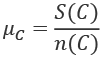
The general definition of the mean is the sum of all of the values divided by the number of values. It's often written like this:

We've defined some set of data, C, as a sequence of n individual values, ![]() . The
. The mean of this collection, ![]() , is the sum of the values divided by the number of values,
, is the sum of the values divided by the number of values, n.
There's a tiny change in this definition that helps to generalize the approach so we can work with Counter objects:


The value of S(C) is the sum of the values. The value of n(C) is the sum using one instead of each value. In effect, S(C) is the sum of ![]() and n(C) is the sum of
and n(C) is the sum of ![]() . We can implement these two computations using the built-in
. We can implement these two computations using the built-in sum() function.
We can reuse these definitions in a number of places. Specifically, we can now define the mean, ![]() , like this:
, like this:
We will use this general idea to provide statistical calculations on data that's part of a Counter object. Instead of a collection of raw values, a Counter object has the raw values and frequencies. The data structure can be described like this:

Each unique value, ![]() , is paired with a frequency,
, is paired with a frequency, ![]() . This makes two small changes to perform similar calculations for S(F) and n(F):
. This makes two small changes to perform similar calculations for S(F) and n(F):


We've defined S(F) to use the product of frequency and value. Similarly, we've defined n(F) to use the frequencies.
In the Using the statistics library recipe, earlier in this chapter, we used a source of data that had a number of Series. Each Series had a name and a number of individual data Point instances.
Here's an overview of each Series and a list of Point data types:
Point = Dict[str, float]
class Series(TypedDict):
    series: str
    data: List[Point]
We've used typing.TypedDict to describe the Series dictionary object. It will have exactly two keys, series and data. The series key will have a string value and the data key will have a list of Point objects as the value.
These types are different from the types shown in the Using the statistics library recipe shown earlier in this chapter. These types reflect a more limited use for the Series object.
For this recipe, a Series object can be summarized by the following function:
def data_counter(
        series: Series, variable_name: str) -> Counter[float]:
    return collections.Counter(
        item[variable_name]
        for item in cast(List[Point], series["data"])
    )
This creates a Counter instance from one of the variables in the Series. In this recipe, we'll look at creating useful statistical summaries from a Counter object instead of a list of raw values.
How to do it...
We'll define a number of small functions that compute sums from Counter objects. We'll then combine these into useful statistics:
- Define the sum of a
Counterobject:def counter_sum(counter: Counter[float]) -> float: return sum(f*v for v, f in counter.items()) - Define the total number of values in a
Counterobject:def counter_len(counter: Counter[float]) -> int: return sum(f for v, f in counter.items()) - We can now combine these to compute a
meanof data that has been put into bins:def counter_mean(counter: Counter[float]) -> float: return counter_sum(counter)/counter_len(counter)
We can use this function with Counter, like this:
>>> s_4_x
Counter({8.0: 10, 19.0: 1})
>>> print(
...     f"Series IV, variable x: "
...     f"mean={counter_mean(s_4_x)}"
... )
Series IV, variable x: mean=9.0
This shows how a Counter object can have essential statistics computed.
How it works...
A Counter is a dictionary. The keys of this dictionary are the actual values being counted. The values in the dictionary are the frequencies for each item. This means that the items() method will produce value and frequency information that can be used by our calculations.
We've transformed each of the definitions for S(F) and S(F) into sums of values created by generator expressions. Because Python is designed to follow the mathematical formalisms closely, the code follows the math in a relatively direct way.
There's more...
To compute the variance (and standard deviation), we'll need two more variations on this theme. We can define an overall mean of a frequency distribution, ![]() :
:

Here, ![]() is the key from the
is the key from the Counter object, F, and ![]() is the frequency value for the given key from the
is the frequency value for the given key from the Counter object.
The variance, ![]() , can be defined in a way that depends on the mean,
, can be defined in a way that depends on the mean, ![]() . The formula is this:
. The formula is this:
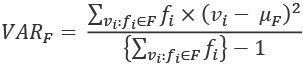
This computes the difference between each distinct value, ![]() , and the mean,
, and the mean, ![]() . This is weighted by the number of times this value occurs,
. This is weighted by the number of times this value occurs, ![]() . The sum of these weighted differences is divided by the count, minus one.
. The sum of these weighted differences is divided by the count, minus one.
The standard deviation, ![]() , is the square root of the variance:
, is the square root of the variance:
![]()
This version of the standard deviation is quite stable mathematically, and therefore is preferred. It requires two passes through the data, which can be better than an erroneous result.
Another variation on the calculation does not depend on the mean, ![]() . This isn't as mathematically stable as the previous version. This variation separately computes the sum of squares of values, the sum of the values, and the count of the values:
. This isn't as mathematically stable as the previous version. This variation separately computes the sum of squares of values, the sum of the values, and the count of the values:

This requires one extra sum computation. We'll need to compute the sum of the values squared, 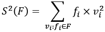 :
:
def counter_sum_2(counter: Counter[float]) -> float:
    return sum(f*v**2 for v, f in counter.items())
Given these three sum functions, ![]() ,
, ![]() , and
, and ![]() , we can define the
, we can define the variance for a Counter with values and frequencies, F:
def counter_variance(counter: Counter[float]) -> float:
   n = counter_len(counter)
   return (
       1/(n-1) *
       (counter_sum_2(counter) - (counter_sum(counter)**2)/n)
   )
The counter_variance() function fits the mathematical definition very closely, giving us reason to believe it's correct.
Using the counter_variance() function, we can compute the standard deviation:
import math
def counter_stdev(counter: Counter[float]) -> float:
   return math.sqrt(counter_variance(counter))
This allows us to see the following:
>>> counter_variance(series_4_x)
11.0
>>> round(counter_stdev(series_4_x), 2)
3.32
These small summary functions for counting, summing, and summing squares provide us with ways to perform simple data analysis without building large collections of raw data. We can work with smaller collections of summary data using Counter objects.
See also
- In the Designing classes with lots of processing recipe in Chapter 7, Basics of Classes and Objects, we looked at this from a slightly different perspective. In that recipe, our objective was simply to conceal a complex data structure.
- The Analyzing many variables in one pass recipe, later in this chapter, will address some efficiency considerations. In that recipe, we'll look at ways to compute multiple sums in a single pass through the data elements.
Computing the coefficient of a correlation
In the Using the built-in statistics library and Average of values in a counter recipes in this chapter, we looked at ways to summarize data. These recipes showed how to compute a central value, as well as variance and extrema.
Another common statistical summary involves the degree of correlation between two sets of data. One commonly used metric for correlation is called Pearson's r. The r-value is the number between -1 and +1 that expresses the degree to which the data values correlate with one another.
A value of zero says the data is random. A value of 0.95 suggests that 95% of the values correlate, and 5% don't correlate well. A value of -0.95 says that 95% of the values have an inverse correlation: when one variable increases, the other decreases.
This is not directly supported by Python's standard library. We can follow a design pattern similar to those shown in the Average of values in a counter recipe, and decompose the larger computation into isolated pieces.
Getting ready
One expression for Pearson's r is this:

We've slightly simplified the summation notation. Instead of  , we've written only
  , assuming the range if the index is clear from the context.
This definition of correlation relies on a large number of individual summations of various parts of a dataset. Each of the ![]() operators can be implemented via the Python
operators can be implemented via the Python sum() function with one of three transformations applied to the value:
sum(1 for x in X)computes a count, shown as n in the definition of Pearson's r.sum(x for x in X)computes the expected sum, and can be simplified tosum(X), shown as and
and  in the preceding equation.
sum(x**2 for x in X)computes the sum of squares, shown as and
and  in the preceding equation.
sum(x*y for x, y in zip(X, Y))computes the sum of products, shown as .
.
We'll use data from the Using the built-in statistics library recipe earlier in this chapter. This data is composed of several individual Series; each Series object is a dictionary with two keys. The series key is associated with a name. The data key is associated with the list of individual Point objects. The following type definitions apply:
from typing import Iterable, TypedDict, List
class Point(TypedDict):
    x: float
    y: float
class Series(TypedDict):
    series: str
    data: List[Point]
These definitions can rely on typing.TypedDict because each reference to a Series object as well as each reference to a Point object uses string literal values that can be matched against the attributes by the mypy tool.
We can read this data with the following command:
>>> from pathlib import Path
>>> import json
>>> source_path = Path('code/anscombe.json')
>>> data: List[Series] = json.loads(source_path.read_text())
We've defined the Path to the data file. We can then use the Path object to read the text from this file. This text is used by json.loads() to build a Python object from the JSON data.
The overall JSON document is a list of Series dictionaries. The data key is associated with a List[Point] object. Each Point object is a dictionary with two keys, x and y. The data looks like this:
    [
      {
        "series": "I",
        "data": [
          {
            "x": 10.0,
            "y": 8.04
          },
          {
            "x": 8.0,
            "y": 6.95
          },
          ...
        ]
      },
      ...
    ]
This set of data has a sequence of Series instances. We'd like to see whether the x and y values correlate with one another by computing the Pearson's coefficient of correlation.
How to do it...
We'll build a number of small sum-related functions first. Given this pool of functions, we can then combine them to create the necessary correlation coefficient:
- Identify the various kinds of summaries required. For the definition, shown above in the Getting ready section of this recipe, we see the following:
- Import the
sqrt()function from themathmodule:from math import sqrt - Define a function that wraps the calculation:
def correlation(series: List[Point]) -> float: - Write the various sums using the built-in
sum()function. This is indented within the function definition. We'll use the value of theseriesparameter: a sequence of values from a givenseries. When we usemypyto check the code, it will try to confirm that the source data fits theTypedDictdefinition, having keysxandy:sumxy = sum(p["x"] * p["y"] for p in series) sumx = sum(p["x"] for p in series) sumy = sum(p["y"] for p in series) sumx2 = sum(p["x"] ** 2 for p in series) sumy2 = sum(p["y"] ** 2 for p in series) n = sum(1 for p in series) - Write the final calculation of r based on the various sums:
    r = (n * sumxy - sumx * sumy) / (
        sqrt(n*sumx2 - sumx**2) * sqrt(n*sumy2 – sumy**2)
    )
    return r
 . This is the count of values. This can also be thought of as
  to be consistent


We can now use this to determine the degree of correlation between the various series:
>>> data = json.loads(source_path.read_text())
>>> for series in data:
...    r = correlation(series['data'])
...    print(f"{series['series']:>3s}, r={r:.2f}")
The output looks like this:
  I, r=0.82
 II, r=0.82
III, r=0.82
 IV, r=0.82
All four series have approximately the same coefficient of correlation. This doesn't mean the series are related to one another. It means that within each series, 82% of the x values predict a y value. This is almost exactly 9 of the 11 values in each series. The four series present interesting case studies in statistical analysis because the details are clearly distinct, but the summary statistics are similar.
How it works...
The overall formula looks rather complex. However, it decomposes into a number of separate sums and a final calculation that combines the sums. Each of the sum operations can be expressed very succinctly in Python.
Conventional mathematical notation might look like the following:

This translates to Python in a very direct way:
sum(p['x'] for p in data)
We can replace each complex-looking ![]() with the slightly more Pythonic variable,
with the slightly more Pythonic variable, ![]() . This pattern can be followed to create
. This pattern can be followed to create ![]() ,
, ![]() ,
, ![]() , and
, and ![]() . These can make it easier to see the overall form of the equation:
. These can make it easier to see the overall form of the equation:

While the correlation() function defined above follows the formula directly, the implementation shown isn't optimal. It makes six separate passes over the data to compute each of the various reductions. As a proof of concept, this implementation works well. This implementation has the advantage of demonstrating that the programming works. It also serves as a starting point for creating unit tests and refactoring the algorithm to optimize the processing.
There's more...
The algorithm, while clear, is inefficient. A more efficient version would process the data once instead of repeatedly computing different kinds of sums. To do this, we'll have to write an explicit for statement that makes a single pass through the data. Within the body of the for statement, the various sums are computed.
An optimized algorithm looks like this:
def corr2(series: List[Point]) -> float:
    sumx = sumy = sumxy = sumx2 = sumy2 = n = 0.0
    for point in series:
        x, y = point["x"], point["y"]
        n += 1
        sumx += x
        sumy += y
        sumxy += x * y
        sumx2 += x ** 2
        sumy2 += y ** 2
    r = (n * sumxy - sumx * sumy) / (
        sqrt(n*sumx2 - sumx**2) * sqrt(n*sumy2 – sumy**2)
    )
    return r
We've initialized a number of results to zero, and then accumulated values into these results from a source of data items, data. Since this uses the data value once only, this will work with any Iterable data source.
The calculation of r from the sums doesn't change. The computation of the sums, however, can be streamlined.
What's important is the parallel structure between the initial version of the algorithm and the revised version that has been optimized to compute all of the summaries in one pass. The clear symmetry of the two versions helps validate two things:
- The initial implementation matches the rather complex formula.
- The optimized implementation matches the initial implementation and the complex formula.
This symmetry, coupled with proper test cases, provides confidence that the implementation is correct.
See also…
- The Computing regression parameters recipe, later in this chapter, will exploit the coefficient of correlation to create a linear model that can be used to predict values of the dependent variable.
- The Analyzing many variables in one pass recipe, later in this chapter, will address some efficiency considerations. In that recipe, we'll look at ways to compute multiple sums in a single pass through the data elements.
Computing regression parameters
Once we've determined that two variables have some kind of relationship, the next step is to determine a way to estimate the dependent variable from the value of the independent variable. With most real-world data, there are a number of small factors that will lead to random variation around a central trend. We'll be estimating a relationship that minimizes these errors, striving for a close fit.
In the simplest cases, the relationship between variables is linear. When we plot the data points, they will tend to cluster around a line. In other cases, we can adjust one of the variables by computing a logarithm or raising it to a power to create a linear model. In more extreme cases, a polynomial is required. The process of linear regression estimates a line that will fit the data with the fewest errors.
In this recipe, we'll show how to compute the linear regression parameters between two variables. This will be based on the correlation computed in Computing the coefficient of correlation recipe earlier in this chapter.
Getting ready
The equation for an estimated line is this:
Given the independent variable, x, the estimated or predicted value of the dependent variable, y, is computed from the ![]() and
and ![]() parameters.
parameters.
The goal is to find values of ![]() and
and ![]() that produce the minimal overall error between the estimated values, y, and the actual values for y. Here's the computation of
that produce the minimal overall error between the estimated values, y, and the actual values for y. Here's the computation of ![]() :
:

Where ![]() is the correlation coefficient. See the Computing the coefficient of correlation recipe earlier in this chapter. The definition of
is the correlation coefficient. See the Computing the coefficient of correlation recipe earlier in this chapter. The definition of ![]() is the standard deviation of
is the standard deviation of x. This value is given directly by the statistics.stdev() function.
Here's the computation of ![]() :
:
Here, ![]() is the
is the mean of y, and ![]() is the
is the mean of x. This, also, is given directly by the statistics.mean() function.
We'll use data from the Using the built-in statistics library recipe earlier in this chapter. This data is composed of several individual Series; each Series object is a dictionary with two keys. The series key is associated with a name. The data key is associated with a list of individual Point objects. The following type definitions apply:
from typing import TypedDict, List
class Point(TypedDict):
    x: float
    y: float
class Series(TypedDict):
    series: str
    data: List[Point]
These definitions can rely on typing.TypedDict because each reference to a Series object, as well as each reference to a Point object, uses string literal values that can be matched against the attributes by the mypy tool.
We can read this data with the following command:
>>> from pathlib import Path
>>> import json
>>> source_path = Path('code/anscombe.json')
>>> data: List[Series] = json.loads(source_path.read_text)
We've defined the Path to the data file. We can then use the Path object to read the text from this file. This text is used by json.loads() to build a Python object from the JSON data.
This set of data has a sequence of Series instances. We'd like to compute the parameters for a linear model that predicts the y value given an x value.
How to do it...
We'll start by leveraging the correlation() function defined in the Computing the coefficient of correlation recipe earlier in this chapter. We'll use this to compute the regression parameters for a linear model:
- Import the
correlation()function and thePointtype hint from the earlier recipe. We'll also need functions from thestatisticsmodule, as well as some common type hints:import statistics from typing import Iterable, TypedDict, List, NamedTuple from Chapter_15.ch15_r03 import correlation, Point - Define a type hint for the regression parameters. This is a tuple to keep the
alphaandbetavalues together:class Regression(NamedTuple): alpha: float beta: float - Define a function that will produce the regression model parameters,
regression(). This will return a two-tuple with thealphaandbetavalues:def regression(series: List[Point]) -> Regression: - Compute the various measures required:
m_x = statistics.mean(p["x"] for p in series) m_y = statistics.mean(p["y"] for p in series) s_x = statistics.stdev(p["x"] for p in series) s_y = statistics.stdev(p["y"] for p in series) r_xy = correlation(series) - Compute the
 and
and  values, and create the regression two-tuple.
    b = r_xy * s_y / s_x
    a = m_y - b * m_x
    return Regression(a, b)
We can use this regression() function to compute the regression parameters as follows:
>>> data = json.loads(source_path.read_text())
>>> for series in data:
...    a, b = regression(series['data'])
...    print(
...        f"{series['series']:>3s} "
...        f"y={round(a, 2)}+{round(b,3)}*x"
...    )
The output shows the formula that predicts an expected y value from a given x value. The output looks like this:
  I y=3.0+0.5*x
 II y=3.0+0.5*x
III y=3.0+0.5*x
 IV y=3.0+0.5*x
In all cases, the equations are ![]() . This estimation appears to be a pretty good predictor of the actual values of y. The four data series were designed to have similar linear regression parameters in spite of having wildly different individual values.
. This estimation appears to be a pretty good predictor of the actual values of y. The four data series were designed to have similar linear regression parameters in spite of having wildly different individual values.
How it works...
The two target formulas for ![]() and
and ![]() are not complex. The formula for
are not complex. The formula for ![]() decomposes into the correlation value used with two standard deviations. The formula for
decomposes into the correlation value used with two standard deviations. The formula for ![]() uses the
uses the ![]() value and two means. Each of these is part of a previous recipe. The correlation calculation contains the actual complexity.
value and two means. Each of these is part of a previous recipe. The correlation calculation contains the actual complexity.
The core design technique is to build new features using as many existing features as possible. This spreads the test cases around so that the foundational algorithms are used (and tested) widely.
The analysis of the performance of Computing the coefficient of a correlation recipe is important, and applies here, as well. The regression() function makes five separate passes over the data to get the correlation as well as the various means and standard deviations. For large collections of data, this is a punishing computational burden. For small collections of data, it's barely measurable.
As a kind of proof of concept, this implementation demonstrates that the algorithm will work. It also serves as a starting point for creating unit tests. Given a working algorithm, then, it makes sense to refactor the code to optimize the processing.
There's more...
The regression algorithm shown earlier, while clear, is inefficient. In order to process the data once, we'll have to write an explicit for statement that makes a single pass through the data. Within the body of the for statement, we can compute the various sums required. Once the sums are available, we can compute values derived from the sums, including the mean and standard deviation:
def regr2(series: Iterable[Point]) -> Regression:
    sumx = sumy = sumxy = sumx2 = sumy2 = n = 0.0
    for point in series:
        x, y = point["x"], point["y"]
        n += 1
        sumx += x
        sumy += y
        sumxy += x * y
        sumx2 += x ** 2
        sumy2 += y ** 2
    m_x = sumx / n
    m_y = sumy / n
    s_x = sqrt((n * sumx2 - sumx ** 2) / (n * (n - 1)))
    s_y = sqrt((n * sumy2 - sumy ** 2) / (n * (n - 1)))
    r_xy = (n * sumxy - sumx * sumy) / (
        sqrt(n * sumx2 - sumx ** 2) * sqrt(n * sumy2 - sumy ** 2)
    )
    b = r_xy * s_y / s_x
    a = m_y - b * m_x
    return Regression(a, b)
We've initialized a number of sums to zero, and then accumulated values into these sums from a source of data items, data. Since this uses the data value once only, this will work with any Iterable data source.
The calculation of r_xy from these sums doesn't change from the previous examples, nor does the calculation of the ![]() or
or ![]() values,
values, ![]() and
and ![]() . Since these final results are the same as the previous version, we have confidence that this optimization will compute the same answer, but do it with only one pass over the data.
. Since these final results are the same as the previous version, we have confidence that this optimization will compute the same answer, but do it with only one pass over the data.
See also
- The Computing the coefficient of correlation recipe earlier in this chapter, provides the
correlation()function that is the basis for computing the model parameters. - The Analyzing many variables in one pass recipe, later in this chapter, will address some efficiency considerations. In that recipe, we'll look at ways to compute multiple sums in a single pass through the data elements.
Computing an autocorrelation
In many cases, events occur in a repeating cycle. If the data correlates with itself, this is called an autocorrelation. With some data, the interval may be obvious because there's some visible external influence, such as seasons or tides. With some data, the interval may be difficult to discern.
If we suspect we have cyclic data, we can leverage the correlation() function from the Computing the coefficient of correlation recipe, earlier in this chapter, to compute an autocorrelation.
Getting ready
The core concept behind autocorrelation is the idea of a correlation through a shift in time, T. The measurement for this is sometimes expressed as ![]() : the correlation between x and x with a time shift of T.
: the correlation between x and x with a time shift of T.
Assume we have a handy correlation function, ![]() . It compares two sequences of length n,
. It compares two sequences of length n, ![]() and
and ![]() , and returns the coefficient of correlation between the two sequences:
, and returns the coefficient of correlation between the two sequences:

We can apply this to autocorrelation by using it as a time shift in the index values:

We've computed the correlation between values of x where the indices are offset by T. If T = 0, we're comparing each item with itself; the correlation is ![]()
We'll use some data that we suspect has a seasonal signal in it. This is data from http://www.esrl.noaa.gov/gmd/ccgg/trends/. We can visit ftp://ftp.cmdl.noaa.gov/ccg/co2/trends/co2_mm_mlo.txt to download the file of the raw data.
The file has a preamble with lines that start with #. These lines must be filtered out of the data. We'll use the Picking a subset – three ways to filter recipe in online Chapter 9, Functional Programming Features (link provided in the Preface), that will remove the lines that aren't useful.
The remaining lines are in seven columns with spaces as the separators between values. We'll use the Reading delimited files with the CSV module recipe in Chapter 10, Input/Output, Physical Format, and Logical Layout, to read CSV data. In this case, the comma in CSV will be a space character. The result will be a little awkward to use, so we'll use the Refactoring a csv DictReader to a dataclass reader recipe in Chapter 10, Input/Output, Physical Format, and Logical Layout, to create a more useful namespace with properly converted values.
To read the CSV-formatted files, we'll need the CSV module as well as a number of type hints:
import csv
from typing import Iterable, Iterator, Dict
Here are two functions to handle the essential aspects of the physical format of the file. The first is a filter to reject comment lines; or, viewed the other way, pass non-comment lines:
def non_comment_iter(source: Iterable[str]) -> Iterator[str]:
    for line in source:
        if line[0] == "#":
            continue
        yield line
The non_comment_iter() function will iterate through the given source of lines and reject lines that start with #. All other lines will be passed untouched.
The non_comment_iter() function can be used to build a CSV reader that handles the lines of valid data. The reader needs some additional configuration to define the data columns and the details of the CSV dialect involved:
def raw_data_iter(
        source: Iterable[str]) -> Iterator[Dict[str, str]]:
    header = [
        "year",
        "month",
        "decimal_date",
        "average",
       "interpolated",
        "trend",
        "days",
    ]
    rdr = csv.DictReader(
        source, header, delimiter=" ", skipinitialspace=True)
    return rdr
The raw_data_iter() function defines the seven column headers. It also specifies that the column delimiter is a space, and the additional spaces at the front of each column of data can be skipped. The input to this function must be stripped of comment lines, generally by using a filter function such as non_comment_iter().
The results of using these two functions are rows of data in the form of dictionaries with seven keys. These rows look like this:
    [{'average': '315.71', 'days': '-1', 'year': '1958', 'trend': '314.62',
        'decimal_date': '1958.208', 'interpolated': '315.71', 'month': '3'},
     {'average': '317.45', 'days': '-1', 'year': '1958', 'trend': '315.29',
        'decimal_date': '1958.292', 'interpolated': '317.45', 'month': '4'},
    etc.
Since the values are all strings, a pass of cleansing and conversion is required. Here's a row cleansing function that can be used in a generator to build a useful NamedTuple:
from typing import NamedTuple
class Sample(NamedTuple):
    year: int
    month: int
    decimal_date: float
    average: float
    interpolated: float
    trend: float
    days: int
def cleanse(row: Dict[str, str]) -> Sample:
    return Sample(
        year=int(row["year"]),
        month=int(row["month"]),
        decimal_date=float(row["decimal_date"]),
        average=float(row["average"]),
        interpolated=float(row["interpolated"]),
        trend=float(row["trend"]),
        days=int(row["days"]),
    )
This cleanse() function will convert each dictionary row to a Sample by applying a conversion function to the values in the raw input dictionary. Most of the items are floating-point numbers, so the float() function is used. A few of the items are integers, and the int() function is used for those.
We can write the following kind of generator expression to apply this cleansing function to each row of raw data:
cleansed_data = (cleanse(row) for row in raw_data)
This will apply the cleanse() function to each row of data. Generally, the expectation is that the rows ready for cleansing will come from the raw_data_iter() generator. Each of these raw rows comes from the non_coment_iter() generator.
These functions can be combined into a stack as follows:
def get_data(source_file: TextIO) -> Iterator[Sample]:
    non_comment_data = non_comment_iter(source_file)
    raw_data = raw_data_iter(non_comment_data)
    cleansed_data = (cleanse(row) for row in raw_data)
    return cleansed_data
This generator function binds all of the individual steps into a transformation pipeline. The non_comment_iter() function cleans out non-CSV lines. The raw_data_iter() function extracts dictionaries from the CSV source. The final generator expression applies the cleanse() function to each row to build Sample objects. We can add filters, or replace the parsing or cleansing functions in this get_data() function.
The context for using the get_data() function will look like this:
>>> source_path = Path('data/co2_mm_mlo.txt')
>>> with source_path.open() as source_file:
...     all_data = list(get_data(source_file))
This will create a List[Sample] object that starts like this:
[Sample(year=1958, month=3, decimal_date=1958.208, average=315.71, interpolated=315.71, trend=314.62, days=-1),
Sample(year=1958, month=4, decimal_date=1958.292, average=317.45, interpolated=317.45, trend=315.29, days=-1),
Sample(year=1958, month=5, decimal_date=1958.375, average=317.5, interpolated=317.5, trend=314.71, days=-1),
…
]
Once we have the raw data, we can use this for statistical processing. We can combine this input pipeline with recipes shown earlier in this chapter to determine the autocorrelation among samples.
How to do it...
To compute the autocorrelation, we'll need to gather the data, select the relevant variables, and then apply the correlation() function:
- Import the
correlation()function from thech15_r03module:from Chapter_15.ch15_r03 import correlation, Point - Get the relevant time series data item from the source data. In this case, we'll use the interpolated data. If we try to use the average data, there are reporting gaps that would force us to locate periods without the gaps. The interpolated data has values to fill in the gaps:
source_path = Path("data") / "co2_mm_mlo.txt" with source_path.open() as source_file: co2_ppm = list( row.interpolated for row in get_data(source_file)) print(f"Read {len(co2_ppm)} Samples") - For a number of time offsets,
 , compute the correlation. We'll use time offsets from
 1to20periods. Since the data is collected monthly, we suspect that will have the highest correlation.
 - The
correlation()function from the Computing the coefficient of correlation recipe expects a small dictionary with two keys: x and y. The first step is to build an array of these dictionaries. We've used thezip()function to combine two sequences of data:co2_ppm[:-tau]co2_ppm[tau:]
- For different
tauoffsets from1to20months, we can create parallel sequences of data and correlate them:for tau in range(1, 20): data = [ Point({"x": x, "y": y}) for x, y in zip(co2_ppm[:-tau], co2_ppm[tau:]) ] r_tau_0 = correlation(data[:60]) r_tau_60 = correlation(data[60:120]) print(f"r_{{xx}}(τ={tau:2d}) = {r_tau_0:6.3f}")
We've taken just the first 60 values to compute the autocorrelation with various time offset values. The data is provided monthly. The strongest correlation is among values that are 12 months apart. We've highlighted this row of output:
    r_{xx}(τ= 1) =  0.862
    r_{xx}(τ= 2) =  0.558
    r_{xx}(τ= 3) =  0.215
    r_{xx}(τ= 4) = -0.057
    r_{xx}(τ= 5) = -0.235
    r_{xx}(τ= 6) = -0.319
    r_{xx}(τ= 7) = -0.305
    r_{xx}(τ= 8) = -0.157
    r_{xx}(τ= 9) =  0.141
    r_{xx}(τ=10) =  0.529
    r_{xx}(τ=11) =  0.857
    r_{xx}(τ=12) =  0.981
    r_{xx}(τ=13) =  0.847
    r_{xx}(τ=14) =  0.531
    r_{xx}(τ=15) =  0.179
    r_{xx}(τ=16) = -0.100
    r_{xx}(τ=17) = -0.279
    r_{xx}(τ=18) = -0.363
    r_{xx}(τ=19) = -0.349
When the time shift is 12, ![]() . A similarly striking autocorrelation is available for almost any subset of the data. This high correlation confirms an annual cycle to the data.
. A similarly striking autocorrelation is available for almost any subset of the data. This high correlation confirms an annual cycle to the data.
The overall dataset contains almost 700 samples spanning over 58 years. It turns out that the seasonal variation signal is not as clear over the entire span of time as it is in the first 5 years' worth of data. This means that there is another, longer period signal that is drowning out the annual variation signal.
The presence of this other signal suggests that something more complex is going on with a timescale longer than 5 years. Further analysis is required.
How it works...
One of the elegant features of Python is the slicing concept. In the Slicing and dicing a list recipe in Chapter 4, Built-In Data Structures Part 1: Lists and Sets, we looked at the basics of slicing a list. When doing autocorrelation calculations, array slicing gives us a wonderful tool for comparing two subsets of the data with very little complexity.
The essential elements of the algorithm amounted to this:
data = [
    Point({"x": x, "y": y})
    for x, y in zip(co2_ppm[:-tau], co2_ppm[tau:])
]
The pairs are built from the zip() function, combing pairs of items from two slices of the co2_ppm sequence. One slice, co2_ppm[:-tau], starts at the beginning, and the other slice, co2_ppm[tau:], starts at an offset. These two slices build the expected (x,y) pairs that are used to create a temporary object, data. Given this data object, an existing correlation() function computed the correlation metric.
There's more...
We can observe the 12-month seasonal cycle repeatedly throughout the dataset using a similar array slicing technique. In the example, we used this:
r_tau_0 = correlation(data[:60])
The preceding code uses the first 60 samples of the available 699. We could begin the slice at various places and use various sizes of the slice to confirm that the cycle is present throughout the data.
We can create a model that shows how the 12 months of data behave. Because there's a repeating cycle, the sine function is the most likely candidate for a model. We'd be having a fit using this:

The mean of the sine function itself is zero, so the K factor is the mean of a given 12-month period. The function, ![]() , will convert monthly figures to proper values in the range
, will convert monthly figures to proper values in the range ![]() . A function such as
. A function such as ![]() might be ideal for this conversion from period to radians. Finally, the scaling factor, A, scales the data to match the minimum and maximum for a given month.
might be ideal for this conversion from period to radians. Finally, the scaling factor, A, scales the data to match the minimum and maximum for a given month.
Long-term model
This analysis exposes the presence of a long-term trend that obscures the annual oscillation. To locate that trend, it is necessary to reduce each 12-month sequence of samples to a single, annual, central value. The median, or the mean, will work well for this.
We can create a sequence of monthly average values using the following generator expression:
from statistics import mean, median
monthly_mean = [
    Point(
        {"x": x, "y": mean(co2_ppm[x : x + 12])}
    )
    for x in range(0, len(co2_ppm), 12)
]
This generator builds a sequence of dictionaries. Each dictionary has the required x and y items that are used by the regression function. The x value is a simple surrogate for the year and month: it's a number that grows from 0 to 696. The y value is the average of 12 monthly values for a given year.
The regression calculation is done as follows:
from Chapter_15.ch15_r04 import regression
alpha, beta = regression(monthly_mean)
print(f"y = {alpha}+x*{beta}")
This shows a pronounced line, with the following equation:

The x value is a month number offset from the first month in the dataset, which is March 1958. For example, March of 1968 would have an x value of 120. The yearly average CO2 parts per million would be y = 323.1. The actual average for this year was 323.27. As you can see, these are very similar values.
The r2 value for this model, which shows how the equation fits the data, is 0.98. This rising slope is the strongest part of the signal, which, in the long run, dominates any seasonal fluctuations.
See also
- The Computing the coefficient of a correlation recipe earlier in this chapter shows the core function for the computing correlation between a series of values.
- The Computing regression parameters recipe earlier in this chapter gives additional background for determining the detailed regression parameters.
Confirming that the data is random – the null hypothesis
One of the important statistical questions is framed as the null hypothesis and an alternate hypothesis about sets of data. Let's assume we have two sets of data, S1 and S2. We can form two kinds of hypothesis in relation to the data:
- Null: Any differences are random effects and there are no significant differences.
- Alternate: The differences are statistically significant. Generally, we consider that the likelihood of this happening stochastically to samples that only differ due to random effects must be less than 5% for us to deem the difference "statistically significant."
This recipe will show one of many ways in which to evaluate data to see whether it's truly random or whether there's some meaningful variation.
Getting ready
The rare individual with a strong background in statistics can leverage statistical theory to evaluate the standard deviations of samples and determine whether there is a significant difference between two distributions. The rest of us, who are potentially weak in statistical theory, but have a strong background in programming, can do a little coding and achieve similar results.
The idea is to generate (or select) either a random subset of the data, or create a simulation of the process. If the randomized data matches the carefully gathered data, we should consider the null hypothesis, and try to find something else to measure. If the measurements don't match a randomized simulation, this can be a useful insight.
There are a variety of ways in which we can compare sets of data to see whether they're significantly different. The Computing the coefficient of correlation recipe from earlier in this chapter shows how we can compare two sets of data for correlation.
A simulation works best when a simulation is reasonably complete. Discrete events in casino gambling, for example, are easy to simulate. Some kinds of discrete events in web transactions, such as the items in a shopping cart, are also easy to simulate. Some phenomena are hard to simulate precisely.
In those cases where we can't do a simulation, we have a number of resampling techniques that are available. We can shuffle the data, use bootstrapping, or use cross-validation. In these cases, we'll use the data that's available to look for random effects.
We'll compare three subsets of the data in the Computing an autocorrelation recipe. We'll reuse the get_data() function to acquire the raw collection of Sample objects.
The context for using the get_data() function will look like this:
>>> source_path = Path('data/co2_mm_mlo.txt')
>>> with source_path.open() as source_file:
...     all_data = list(get_data(source_file))
This will create a List[Sample] objects that starts like this:
[Sample(year=1958, month=3, decimal_date=1958.208, average=315.71, interpolated=315.71, trend=314.62, days=-1),
 Sample(year=1958, month=4, decimal_date=1958.292, average=317.45, interpolated=317.45, trend=315.29, days=-1),
 Sample(year=1958, month=5, decimal_date=1958.375, average=317.5, interpolated=317.5, trend=314.71, days=-1),
…
]
We want subsets of the data. We'll look at data values from two adjacent years and a third year that is widely separated from the other two. Each year has 12 samples, and we can compute the means of these groups:
>>> y1959 = [r.interpolated for r in all_data if r.year == 1959]
>>> y1960 = [r.interpolated for r in all_data if r.year == 1960]
>>> y2014 = [r.interpolated for r in all_data if r.year == 2014]
We've created three subsets for three of the available years of data. Each subset is created with a filter that creates a list of values for which the year matches a target value. We can compute statistics on these subsets as follows:
>>> from statistics import mean
>>> round(mean(y1959), 2)
315.97
>>> round(mean(y1960), 2)
316.91
>>> round(mean(y2014), 2)
398.61
The three mean values are different. Our hypothesis is that the differences between the 1959 and 1960 mean values are insignificant random variation, while the differences between the 1959 and 2014 mean values are statistically significant.
The permutation or shuffling technique for resampling works as follows:
- Start with two collections of points to compare. For example, we can compare the data samples from
1959and1960, and
and  . The observed difference between the means of the
 1959data, , and the 1960 data,
  is
is  . We can call this Tobs, the observed test measurement. We can then compute random subsets to compare arbitrary data to this specific grouping.
 - Combine the data from the two collections into a single population of data points,
 .
. - For each permutation of the population of values, P:
- Create two subsets from the permutation, A, and B, such that
 . This is the resampling step that gives the process its name.
 - Compute the difference between the means of each resampled subset,
 .
. - Count the number of differences, L, larger than Tobs and, S, smaller than Tobs.
- Create two subsets from the permutation, A, and B, such that
If the differences between ![]() and
and ![]() are not statistically significant, all the random subsets of data will be scattered evenly around the observed measurement, Tobs. If there is a statistically significant difference, however, the distribution of random subsets will be highly skewed. A common heuristic threshold is to look for a 20:1 ratio between larger and smaller counts, L, and S.
are not statistically significant, all the random subsets of data will be scattered evenly around the observed measurement, Tobs. If there is a statistically significant difference, however, the distribution of random subsets will be highly skewed. A common heuristic threshold is to look for a 20:1 ratio between larger and smaller counts, L, and S.
The two counts show us how our observed difference compares with all possible differences. There can be many permutations. In our case, we know that the number of combinations of 24 samples taken 12 at a time is given by this formula:
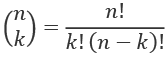
We can compute the value for n = 24 and k = 12:
>>> from Chapter_03.ch03_r10 import fact_s
>>> def binom(n, k):
...     return fact_s(n)//(fact_s(k)*fact_s(n-k))
>>> binom(24, 12)
2704156
There are a fraction more than 2.7 million permutations of 24 values taken 12 at a time. We can use functions in the itertools module to generate these. The combinations() function will emit the various subsets. Processing all these combinations takes over 5 minutes (320 seconds).
An alternative plan is to use randomized subsets. Using 270,415 randomized samples can be done in under 30 seconds on a four-core laptop. Using 10% of the combinations provides an answer that's accurate enough to determine whether the two samples are statistically similar and the null hypothesis is true, or if the two samples are different.
How to do it...
To apply the shuffling technique, we'll leverage the statistics and random modules. We'll compute descriptive statistics for a number of random subsets.
- We'll be using the
randomandstatisticsmodules. Theshuffle()function is central to randomizing the samples. We'll also be using themean()function. While the process suggests two counts, values above and below the observed difference, Tobs, we'll instead create aCounterand quantize the counts in 2,000 fine-grained steps from-0.001to+0.001. This will provide some confidence that the differences are normally distributed:import collections import random from statistics import mean - Define a function that accepts two separate sets of samples. These will be compared using the randomized shuffling procedure:
def randomized( s1: List[float], s2: List[float], limit: int = 270_415) -> None: - Compute the observed difference between the means, Tobs:
T_obs = mean(s2) - mean(s1) print( f"T_obs = {mean(s2):.2f}-{mean(s1):.2f} " f"= {T_obs:.2f}" ) - Initialize a
Counterobject to collect details:counts: Counter[int] = collections.Counter() - Create the combined universe of samples. We can concatenate the two lists:
universe = s1 + s2 - Use a
forstatement to perform a large number of resamples;270,415samples can take35seconds. It's easy to expand or contract the subset to balance a need for accuracy and the speed of calculation. The bulk of the processing will be nested inside this loop:for resample in range(limit): - Shuffle the data:
random.shuffle(universe) - Pick two subsets that match the original sets of data in size. It seems easiest to slice the shuffled data cleanly into two subsets:
a = universe[:len(s2)] b = universe[len(s2):] - Compute the difference between the means. In this case, we'll scale this by
1000and convert to an integer so that we can accumulate a frequency distribution:delta = int(1000*(mean(a) - mean(b))) counts[delta] += 1 - After the
forloop, summarize thecountsshowing how many are above the observed difference, and how many are below it. If either value is less than 5%, this is a statistically significant difference:T = int(1000*T_obs) below = sum(v for k,v in counts.items() if k < T) above = sum(v for k,v in counts.items() if k >= T) print( f"below {below:,} {below/(below+above):.1%}, " f"above {above:,} {above/(below+above):.1%}" )
When we run the randomized() function for the data from 1959 and 1960, we see the following:
print("1959 v. 1960")
randomized(y1959, y1960)
The output looks like the following:
1959 v. 1960
T_obs = 316.91-315.97 = 0.93
below 239,491 88.6%, above 30,924 11.4%
This shows that 11% of the data was above the observed difference, while 88% was below it. This is well within the realm of normal statistical noise.
When we run this for data from 1959 and 2014, we see the following output:
1959 v. 2014
T_obs = 398.61-315.97 = 82.64
below 270,415 100.0%, above 0 0.0%
The data here shows that none of the resampled subsets was above the observed difference in means, Tobs. We can conclude from this resampling exercise that the change from 1959 to 2014 is statistically significant.
How it works...
Computing all 2.7 million permutations gives the exact answer to a comparison of the given subsets with all possible subsets. It's faster to use many randomized subsets instead of computing all possible permutations. The Python random number generator is excellent, and it assures us that the randomized subsets will be fairly distributed.
We've used two techniques to compute randomized subsets of the data:
- Shuffle the entire universe with
random.shuffle(u). - Partition the universe with code similar to
a,b = u[x:],u[:x].
Computing the means of the two partitions is done with the statistics module. We could define somewhat more efficient algorithms that did the shuffling, partitioning, and mean computation all in a single pass through the data.
The preceding algorithm turned each difference into a value between -1000 and +1000 using this:
delta = int(1000*(mean(a) - mean(b)))
This allows us to compute a frequency distribution with a Counter. This will indicate that most of the differences really are zero, something to be expected for normally distributed data. Seeing the distribution assures us that there isn't some hidden bias in the random number generation and shuffling algorithm.
Instead of populating a Counter, we could simply count the above and below values. The simplest form of this comparison between a permutation's difference and the observed difference, Tobs, is as follows:
    if mean(a) - mean(b) > T_obs:
        above += 1
This counts the number of resampling differences that are larger than the observed difference. From this, we can compute the number below the observation via below = limit-above. This will give us a simple percentage value.
There's more...
We can speed processing up a tiny bit more by changing the way we compute the mean of each random subset.
Given a pool of numbers, P, we're creating two disjoint subsets, A, and B, such that:


The union of the A and B subsets covers the entire universe, P. There are no missing values because the intersection between A and B is an empty set.
The overall sum, Sp, can be computed just once:

We only need to compute a sum for one subset, SA:

This means that the other subset sum is a subtraction. We don't need a costly process to compute a second sum.
The sizes of the sets, NA, and NB, similarly, are constant. The means, ![]() and
and ![]() , can be calculated a little more quickly than by using the
, can be calculated a little more quickly than by using the statistics.mean() function:


This leads to a slight change in the resample function. We'll look at this in three parts. First, the initialization:
def faster_randomized(
        s1: List[float],
        s2: List[float],
        limit: int = 270_415) -> None:
    T_obs = mean(s2) - mean(s1)
    print(
        f"T_obs = {mean(s2):.2f}-{mean(s1):.2f} "
        f"= {T_obs:.2f}")
    counts: Counter[int] = collections.Counter()
    universe = s1 + s2
    a_size = len(s1)
    b_size = len(s2)
    s_u = sum(universe)
Three additional variables have been introduced: a_size and b_size are the sizes of the two original sets; s_u is the sum of all of the values in the universe. The sums of each subset must sum to this value, also.
Here's the second part of the function, which performs resamples of the full universe:
    for resample in range(limit):
        random.shuffle(universe)
        a = universe[: len(s1)]
        s_a = sum(a)
        m_a = s_a/a_size
        m_b = (s_u-s_a)/b_size
        delta = int(1000*(m_a-m_b))
        counts[delta] += 1
This resampling loop will compute one subset, and the sum of those values. The sum of the remaining values is computed by subtraction. The means, similarly, are division operations on these sums. The computation of the delta bin into which the difference falls is very similar to the original version.
Here's the final portion to display the results. This has not changed:
    T = int(1000 * T_obs)
    below = sum(v for k, v in counts.items() if k < T)
    above = sum(v for k, v in counts.items() if k >= T)
    print(
        f"below {below:,} {below/(below+above):.1%}, "
        f"above {above:,} {above/(below+above):.1%}"
    )
By computing just one sum, s_a, we shave considerable processing time off of the random resampling procedure. On a small four-core laptop, processing time dropped from 26 seconds to 3.6 seconds. This represents a considerable saving by avoiding computations on both subsets. We also avoided using the mean() function, and computed the means directly from the sums and the fixed counts.
This kind of optimization makes it quite easy to reach a statistical decision quickly. Using resampling means that we don't need to rely on a complex theoretical knowledge of statistics; we can resample the existing data to show that a given sample meets the null hypothesis or is outside of expectations, meaning that an alternative hypothesis is called for.
See also
- This process can be applied to other statistical decision procedures. This includes the Computing regression parameters and Computing an autocorrelation recipes earlier in this chapter.
Locating outliers
A set of measurements may include sample values that can be described as outliers. An outlier deviates from other samples, and may indicate bad data or a new discovery. Outliers are, by definition, rare events.
Outliers may be simple mistakes in data gathering. They might represent a software bug, or perhaps a measuring device that isn't calibrated properly. Perhaps a log entry is unreadable because a server crashed, or a timestamp is wrong because a user entered data improperly. We can blame high-energy cosmic ray discharges near extremely small electronic components, too.
Outliers may also be of interest because there is some other signal that is difficult to detect. It might be novel, or rare, or outside the accurate calibration of our devices. In a web log, this might suggest a new use case for an application or signal the start of a new kind of hacking attempt.
In this recipe, we'll look at one algorithm for identifying potential outliers. Our goal is to create functions that can be used with Python's filter() function to pass or reject outlier values.
Getting ready
An easy way to locate outliers is to normalize the values to make them Z-scores. A Z-score converts the measured value to a ratio between the measured value and the mean measured in units of standard deviation:
Here, ![]() is the mean of a given variable, x, and
is the mean of a given variable, x, and ![]() is the standard deviation of that variable. We can compute the
is the standard deviation of that variable. We can compute the mean and standard deviation values using the statistics module.
This, however, can be somewhat misleading because the Z-scores are limited by the number of samples involved. If we don't have enough data, we may be too aggressive (or too conservative) on rejecting outliers. Consequently, the NIST Engineering and Statistics Handbook, Section 1.3.5.17, suggests using the modified Z-score, ![]() , for detecting outliers:
, for detecting outliers:

Median Absolute Deviation (MAD) is used instead of the standard deviation for this outlier detection. The MAD is the median of the absolute values of the deviations between each sample, ![]() , and the population median,
, and the population median, ![]() :
:

The scaling factor of 0.6745 is used so that an Mi value greater than 3.5 can be identified as an outlier. This modified Z-score uses the population median, parallel to the way Z-scores use the sample variance.
We'll use data from the Using the built-in statistics library recipe shown earlier in this chapter. This data includes several individual Series, where each Series object is a dictionary with two keys. The series key is associated with a name. The data key is associated with a list of individual Point objects. The following type definitions apply:
from typing import Iterable, TypedDict, List, Dict
Point = Dict[str, float]
class Series(TypedDict):
    series: str
    data: List[Point]
The Series definition can rely on typing.TypedDict because each reference to a Series object uses string literal values that can be matched against the attributes by the mypy tool. The references to items within the Point dictionary will use variables instead of literal key values, making it impossible for the mypy tool to check the type hints fully.
We can read this data with the following command:
>>> from pathlib import Path
>>> import json
>>> source_path = Path('code/anscombe.json')
>>> data: List[Series] = json.loads(source_path.read_text)
We've defined the Path to the data file. We can then use the Path object to read the text from this file. This text is used by json.loads() to build a Python object from the JSON data.
This set of data has a sequence of Series instances. Each observation is a pair of measurements in a Point dictionary. In this recipe, we'll create a series of operations to locate outliers in the x or y attribute of each Point instance.
How to do it...
We'll need to start with the median() function of the statistics module. With this to create the threshold, we can build functions to work with the filter() function to pass or reject an outlier:
- Import the
statisticsmodule. We'll be doing a number ofmediancalculations. In addition, we can use some of the features ofitertools, such ascompress()andfilterfalse():import statistics import itertools - Define the
absdev()function to map from absolute values to Z-scores. This will either use a givenmedianor compute the actualmedianof the samples. It will then return a generator that provides all of the absolute deviations from themedian:def absdev( data: Sequence[float], median: Optional[float] = None) -> Iterator[float]: if median is None: median = statistics.median(data) return (abs(x - median) for x in data) - Define a function to compute the
medianof deviations from themedian, themedian_absdev()function. This will locate themedianof a sequence of absolute deviation values. This computes theMADvalue used to detect outliers. This can compute amedianor it can be given amedianalready computed:def median_absdev( data: Sequence[float], median: Optional[float] = None) -> float: if median is None: median = statistics.median(data) return statistics.median(absdev(data, median=median)) - Define the modified Z-score mapping,
z_mod(). This will compute themedianfor the dataset, and use this to compute the MAD. The MAD value is then used to compute modified Z-scores based on this deviation value. The returned value is an iterator over the modified Z-scores. Because multiple passes are made over the data, the input can't be aniterablecollection, so it must be alistobject:def z_mod(data: Sequence[float]) -> Iterator[float]: median = statistics.median(data) mad = median_absdev(data, median) return (0.6745 * (x - median) / mad for x in data)Interestingly, there's a possibility that the MAD value is zero. This can happen when the majority of the values don't deviate from the
median. When more than half of the points have the same value, themedianabsolute deviation will be zero, and it's difficult to detect outliers with this method. - Define two outlier filters based on the modified Z mapping,
pass_outliers(), andreject_outliers(). Any value over 3.5 can be labeled as an outlier. The statistical summaries can then be computed with and without the outlier values. Theitertoolsmodule has acompress()function that can use a sequence ofBooleanselector values to choose items from the original data sequence based on the results of thez_mod()computation:def pass_outliers(data: Sequence[float] ) -> Iterator[float]: return itertools.compress( data, (z >= 3.5 for z in z_mod(data))) def reject_outliers(data: Sequence[float] ) -> Iterator[float]: return itertools.compress( data, (z < 3.5 for z in z_mod(data)))
Most of these functions make multiple references to the input data parameter—an iterable cannot be used. These functions must be given a Sequence object so the data can be examined multiple times.
We can use pass_outliers() to locate the outlier values. This can be handy to identify the suspicious data values. We can use reject_outliers() to provide data with the outliers removed from consideration; this data would be used for other analysis steps.
How it works...
The stack of transformations can be summarized like this:
- Compute the overall population median.
- Map each value to an absolute deviation from the population median.
- Reduce the absolute deviations to create a median absolute deviation, MAD.
- Map each value to the modified Z-score using the population median and the MAD.
- Filter the results based on the modified Z-scores.
We've defined each transformation function in this stack separately. We can use recipes from the online Chapter 9, Functional Programming Features (link provided in the Preface), to create smaller functions and use the built-in map() and filter() functions to implement this process.
We can't easily use the built-in reduce() function to define a median computation. Efficient computation of the median involves a recursive algorithm to partition the data into smaller and smaller subsets, one of which has the median value. A less efficient alternative is to sort the data and choose the value in the middle.
Here's how we can apply the outlier detection to the given sample data:
def examine_all_series(source_path: Path) -> None:
    raw_data: List[Series] = json.loads(source_path.read_text())
    series_map = {
        series["series"]: series["data"]
        for series in raw_data}
    for series_name in series_map:
        print(series_name)
        series_data = series_map[series_name]
        for variable_name in 'x', 'y':
            values = [item[variable_name] for item in series_data]
            print(variable_name, values, end=" ")
            try:
                print("outliers", list(pass_outliers(values)))
            except ZeroDivisionError:
                print("Data Appears Linear")
        print()
We've iterated through each of the series in the source data. The computation of series_data extracts one of the series from the source data. Each of the series is a list of dictionaries with two keys, x and y. Within the set of samples, we can use the pass_outliers() function to locate outliers in the data.
The except clause handles a ZeroDivisionError exception. This exception is raised by the z_mod() function for a particularly pathological set of data. Here's the line of output that shows this odd-looking data:
x [8.0, 8.0, 8.0, 8.0, 8.0, 8.0, 8.0, 19.0, 8.0, 8.0, 8.0] Data Appears Linear
In this case, more than half the values are the same, which leads the mode to also be the median. More than half the absolute deviations from the median will be zero, leaving the MAD to be zero. In this case, the idea of outliers is suspicious because the data doesn't seem to reflect ordinary statistical noise either.
When we find data like this, that does not fit the general model, and a different kind of analysis must be applied. It's possible, for example, that the cluster of identical values represents some kind of measurement error. Those values are invalid, and need to be rejected. This would leave a very small dataset with only a single valid point.
There's more...
The design shown in the recipe used two similar looking function definitions to the pass_outliers() and reject_outliers() functions. This design suffers from an unpleasant duplication of critical program logic; it breaks the DRY principle because a critical computation is repeated. Here are the two functions:
def pass_outliers(data: List[float]) -> Iterator[float]:
    return itertools.compress(
        data, (z >= 3.5 for z in z_mod(data)))
def reject_outliers(data: List[float]) -> Iterator[float]:
    return itertools.compress(
        data, (z < 3.5 for z in z_mod(data)))
The difference between pass_outliers() and reject_outliers() is tiny, and amounts to a logical negation of an expression. We have >= in one version and < in another. If the logic was more complex than a simple comparison, it may be difficult to be certain that the two logical expressions were opposites.
We can extract one version of the filter rule to create something like the following:
outlier = lambda z: z >= 3.5
We can then modify the two uses of the compress() function to make the logical negation explicit:
def pass_outliers_2(data: List[float]) -> Iterator[float]:
    return itertools.compress(
        data, (outlier(z) for z in z_mod(data)))
def reject_outliers_2(data: List[float]) -> Iterator[float]:
    return itertools.compress(
        data, (not outlier(z) for z in z_mod(data)))
The essential rule, outlier(), is like a separate lambda object. This helps reduce the code duplication and makes the logical negation more obvious. Now, the two versions can be compared easily to be sure that they have appropriate behavior.
We've used itertools.compress() to pass or reject outliers. This allows us to have a sequence of Boolean values and a sequence of data values. The function chooses data values where the matching Boolean value is True.
Another possible design alternative is to use the built-in filter() function. This leads to a radical transformation of the processing pipeline. The filter() higher-order function requires a decision function that creates a Boolean result for each raw value. Instead of comparing z_mod() results to a threshold, this version must compute the z_mod() value and also apply the decision threshold in a single function. The decision function for the filter() function is this:
This decision function requires two additional inputs—the population median, x, and the MAD value. This makes the filter decision function rather complex. It would look like this:
def filter_outlier(mad: float, median_x: float, x: float) -> bool:
    return 0.6745*(x - median_x)/mad >= 3.5
This filter_outlier() function can be used with filter() to pass outliers. It can be used with itertools.filterfalse() to reject outliers and create a subset that is free from erroneous values.
In order to use this filter_outlier() function, we'll need to create a pair of functions like these:
from functools import partial
def make_filter_outlier_partial(
        data: List[float]) -> Callable[[float], bool]:
    population_median = statistics.median(data)
    mad = median_absdev(data, population_median)
    outlier_partial = partial(
        filter_outlier, mad, population_median)
    return outlier_partial
def pass_outliers_3(data: List[float]) -> Iterator[float]:
    outlier_partial = make_filter_outlier_partial(data)
    return filter(outlier_partial, data)
The make_filter_outlier_partial() function creates a partial function built around the filter_outlier() function. This partial function provides fixed values for the mad and median_x parameters; the x parameter is the only remaining parameter.
To create the partial function, the make_filter_outlier_partial() function computes the two overall reductions: population_median, and mad. Given these two values, the partial function, outlier_partial() is created with two parameter values bound.
The pass_outliers_3() function is identical to previous pass_outliers() functions. It expects a sequence of data values. First, it creates the necessary partial function, and then it applies the partial function to pass outlier values. A similar function can be defined to reject outliers; the principal difference involves using the itertools.filterfalse() function instead of the built-in filter() function.
See also
- See http://www.itl.nist.gov/div898/handbook/eda/section3/eda35h.htm for details on algorithms that help with the detection of outlier values from a set of measurements.
Analyzing many variables in one pass
In many cases, we'll have data with multiple variables that we'd like to analyze. The data can be visualized as filling in a grid, with each row containing a specific outcome. Each outcome row has multiple variables in columns. Many recipes in this chapter have a very narrow grid with only two variables, x and y. Two recipes earlier in this chapter, Computing an autocorrelation, and Confirming that the data is random – the null hypothesis, have relied on data with more than two variables.
For many of these recipes, we have followed a pattern of treating the data as if it is provided in column-major order: the recipe processed each variable (from a column of data) independently. This leads to visiting each row of data multiple times. For a large number of rows, this can become inefficient.
The alternative is to follow a pattern of row-major order. This means processing all the variables at once for each row of data. This refactoring tends to make the functions a bit more complex-looking, but considerably more efficient.
We'll look at ways to optimize an algorithm to make a single pass through a set of data and collect several descriptive statistics all at once.
Getting ready
The variables that we might want to analyze will fall into a number of categories. For example, statisticians often segregate variables into categories such as the following:
- Continuous real-valued data: These variables are often measured by floating-point values, they have a well-defined unit of measure, and they can take on values with a precision limited by the accuracy of the measurement.
- Discrete or categorical data: These variables take on a value selected from a finite domain. In some cases, we can enumerate the domain in advance. Postal ZIP codes, for example, are often known in advance. In other cases, the domain's values must be discovered.
- Ordinal data: This provides a ranking or ordering. Generally, the ordinal value is a number; no other statistical summaries apply to this number. Since it's not really a measurement, it has no units, for example.
- Count data: This variable is a summary of individual discrete outcomes. It can be treated as if it were continuous by computing a real-valued mean of an otherwise discrete count.
Variables may be independent of each other, or a variable may depend on other variables. In the initial phases of a study, the dependence may not be known. In later phases, one objective of the software is to discover the dependencies. Later, software may be used to model the dependencies.
Because of the varieties of data, we need to treat each variable as a distinct item. We can't treat them all as simple floating-point values. Properly acknowledging the differences will lead to a hierarchy of class definitions. Each subclass will contain the unique features for a variable.
We have two overall design patterns:
- Eager: We can compute the various summaries as early as possible. In some cases, we don't have to accumulate very much data for this.
- Lazy: We compute the summaries as late as possible. This means that we'll be accumulating data, and using properties to compute the summaries.
For very large sets of data, we want to have a hybrid solution. We'll compute some summaries eagerly, and also use properties to compute the final results from those summaries.
We'll use some data from the Using the built-in statistics library recipe earlier in this chapter, and we'll also use some data from the Computing an autocorrelation recipe ealier in this chapter. In both cases, the data is a sequence of dictionaries. Each key is a column name. The values are mostly numbers, but it's a mixture of integer (discrete) values and floating-point (continuous) values.
The following type definitions apply
from typing import TypedDict, List, Dict
Sample = Dict[str, str]
class Series(TypedDict):
    series: str
    data: List[Sample]
The Series definition can rely on typing.TypedDict because each reference to a Series object uses string literal values that can be matched against the attributes by the mypy tool. The references to items within the Point dictionary will use variables instead of literal key values, making it impossible for the mypy tool to check the type hints fully.
This recipe will be designed to work with potentially invalid data. The Sample dictionary definition reflects this by expecting data with string values that will be cleansed and converted to more useful Python objects. We'll include this cleansing step in this recipe.
We can read this data with the following command:
>>> from pathlib import Path
>>> import json
>>> source_path = Path('code/anscombe.json')
>>> data: List[Series] = json.loads(source_path.read_text)
We've defined the Path to the data file. We can then use the Path object to read the text from this file. This text is used by json.loads() to build a Python object from the JSON data.
How can we examine all of the variables in a given series at once? We'll focus on an eager design that can work with very large volumes of data by minimizing the amount of raw data that's used.
How to do it...
We'll define a class that can include a number of summary values. The computations will rely on the data being kept in a separate object that is a collection of raw data. We'll define a hierarchy of classes for the various kinds of summaries:
- Define a superclass for various kinds of analysis. This will act as a superclass for all more specialized analytics classes that may be required. We'll call this class
StatsGatherbecause that seems to summarize the general purpose:from abc import abstractmethod class StatsGather: def __init__(self, name: str) -> None: self.name = name @abstractmethod def add(self, value: Any) -> None: raise NotImplementedError @abstractmethod def summary(self) -> str: raise NotImplementedError - Define a class to handle the analysis of the variable. This should handle all conversions and cleansing. We'll eagerly compute the
count,sum, andsumof squares values that can be used to compute themeanand standard deviation. We won't compute the finalmeanor standard deviation until these property values are requested:import math class SimpleStats(StatsGather): def __init__(self, name: str) -> None: super().__init__(name) self.count = 0 self.sum = 0 self.sum_2 = 0 def cleanse(self, value: Any) -> float: return float(value) def add(self, value: Any) -> None: value = self.cleanse(value) self.count += 1 self.sum += value self.sum_2 += value * value @property def mean(self) -> float: return self.sum / self.count @property def stdev(self) -> float: return math.sqrt( (self.count * self.sum_2 - self.sum ** 2) / (self.count * (self.count - 1)) ) def summary(self) -> str: return ( f"{self.name} " f"mean={self.mean:.1f} stdev={self.stdev:.3f}" ) - Define an
analyze()function that creates multiple instances of theSimpleStatsclass and applies these to columns of data:def analyze( series_data: Iterable[Sample], names: List[str] ) -> Dict[str, SimpleStats]: - Create a mapping from column names to instances of the
SimpleStatsclass. Each of these objects will accumulate the summaries of the matching column of data:column_stats = { key: SimpleStats(key) for key in names } - Define a function to process all rows, using the
statistics-computing objects for each column within eachrow. The outerforstatement processes eachrowof data. The innerforstatement processes each column of eachrow. The processing is clearly inrow-major order:for row in series_data: for column_name in column_stats: column_stats[column_name].add(row[column_name]) return column_stats - Display results or summaries from the various objects. The following snippet requires a
series_name, and adata_streamwhich is aniterableover thePointtypes:print(f"{series_name:>3s} var mean stddev") column_stats = analyze(data_stream, ["x", "y"]) for column_key in column_stats: print(" ", column_stats[column_key].summary())
This gives an overview of each of the variables. We might see output like this for a series named I:
I
x mean=9.0 stdev=3.317
y mean=7.5 stdev=2.032
The analyze() function provides a summary, making a single pass through the data. This can be helpful for immense datasets that don't fit into the computer's memory.
How it works...
We've created the SimpleStats class to handle cleansing, filtering, and statistical processing for a continuous variable with a floating-point value. When confronted with other kinds of variables, for example, a discrete variable, we'll need additional class definitions. The idea is to be able to create a hierarchy of related classes, all of which have the essential StatsGather interface.
The analyze() function created an instance of the SimpleStats class for each specific column that we're going to analyze. For discrete or ordinal data, the computation of mean and standard deviation doesn't make sense, so a different summary object is required.
The StatsGather class is an abstract superclass requiring each subclass to provide an add() method and a summary() method. Each individual data value is provided to the add() method.
A subclass can provide any additional statistics that might be interesting. In this case, the SimpleStats class provided mean and stdev properties to compute summary statistics.
The SimpleStats class also defines an explicit cleanse() method. This can handle the data conversion needs. This can be extended to handle the possibility of invalid data. It might filter the values instead of raising an exception.
The overall analyze() function uses a collection of these SimpleStats statistics-processing objects. As a practical matter, there will be multiple classes involved in handling discrete variables and other kinds of data conversion processing. As each row of data is consumed by the for statement inside the analyze() function, all of the various StatsGather objects in the column_stats dictionary are updated using the add() method.
When all the rows have been consumed, the summaries in the column_stats dictionary can be displayed. This will provide summaries of the available data without loading huge datasets into memory.
There's more...
In this design, we've only considered the case where a variable is continuous and maps to a floating-point value. While this is common, there are a number of other categories of variables. One of the common alternatives is a discrete integer-valued variable.
We'll define an additional class, similar to SimpleStats, to handle this case. For discrete values, there's no good reason to use a measure of central tendency, like a mean or a median. A frequency distribution table, however, can be useful.
Here's a class that uses a collection.Counter object to compute the frequency of each discrete integer value:
class IntegerDiscreteStats:
def __init__(self, name: str) -> None:
self.name = name
self.counts: Counter[int] = collections.Counter()
def cleanse(self, value: Any) -> float:
return int(value)
def add(self, value: Any) -> None:
value = self.cleanse(value)
self.counts[value] += 1
@property
def mode(self) -> Tuple[int, int]:
return self.counts.most_common(1)[0]
@property
def fq_dist(self) -> Counter[int]:
return self.counts
This IntegerDiscreteStats class defines a cleanse() method to convert the source string to an integer. These integer values are then used to populate the self.counts object. The modal value is the most common value in the collection.
A more sophisticated class might check for several values with similar frequencies to expose the fact that the modal value is not unique. We've omitted any checking and simply reported the most common value and the count.
The fq_dist property is a reference to the underlying Counter object. This method isn't required, but this method can help to encapsulate internal processing, separating it from the return type provided by the property.
Our initial analyze() function built a dictionary mapping the column names provided in the names parameter to SimpleStats instances. This is limiting because it makes an assumption that all of the variables in the source data will fit the SimpleStats model. A better design would be to provide the collection of keys and statistical analyzers. A function like this works out better because it makes fewer assumptions about the data being analyzed:
def analyze2(
series_data: Iterable[Sample],
column_stats: Dict[str, StatsGather]
) -> Dict[str, StatsGather]:
    for row in series_data:
        for column_name in column_stats:
            column_stats[column_name].add(row[column_name])
    return column_stats
This function expects to be given a mapping from column names to StatsGather subclass instances. For example:
column_stats: Dict[str, StatsGather] = {
    "year": IntegerDiscreteStats("year"),
    "month":  IntegerDiscreteStats("month"),
    "decimal_date": SimpleStats("decimal_date"),
    "average": SimpleStats("average"),
    "interpolated": SimpleStats("interpolated"),
    "trend": SimpleStats("trend"),
    "days": IntegerDiscreteStats("days"),
}
could be used to analyze the more complex raw data used in the Computing an autocorrelation and Confirming that the data is random – the null hypothesis recipes earlier in this chapter.
See also
- See the Designing classes with lots of processing and Using properties for lazy attributes recipes in Chapter 7, Basics of Classes and Objects, for some additional design alternatives that fit into this overall approach.
- We can make use of the Command Design Patterns as well. See the Combining many applications using the Command Design Pattern section in Chapter 14, Application Integration: Combination, for ways to combine multiple individual
Commandclasses into a compositeCommandclass definition.