
OptML framework and its application to model optimization
Güner Orhan; Mehmet Akşit University of Twente, Computer Science, Formal Methods & Tools Group, Enschede, The Netherlands
Abstract
Model-based software development, in particular Model-Driven Engineering (MDE), has received a lot of attention during the last decade. More and more companies adopt MDE methods in software development. As a consequence, software engineers may need to deal with a large model base which becomes the main company asset. Moreover, there may be many configurations of the same model resulting in a large set of alternatives for the software engineers to take into account. This chapter presents the OptML Framework, which accepts various models defined in the Ecore MDE environment and computes the optimal models which satisfy user-defined constraints. Commonly used models in the MDE context such as class model, feature model, platform model, and process model are utilized in this chapter for illustration purposes. The examples of user-defined criteria are timeliness, energy consumption, and precision. To the best of our knowledge, this is the first generic MDE framework that is suitable for model optimization. The term generic here refers to a tool workbench architecture that is deliberately designed to extend the workbench with new features if necessary. The framework is fully implemented and tested for a selected set of models defined in the image processing domain.
Keywords
Model-Driven Engineering; OptML Framework; model optimization; schedulability analysis; multiquality optimization
9.1 Introduction
Since the 2010s, there has been an increasing emphasis on Model-Driven Engineering (MDE) [1]. There has been a considerable effort in definition and implementation of models in a large category of application domains and as such many useful models are readily available for use.
Availability of models in the domains of interest, however, creates its own problems to deal with.
First, due to complexity of the domain of interest, complexity and size of models can be very large [2]. Although there have been some approaches, such as model splitting/merging/transforming [3], which can be used to deal with model complexity, generally they must be “hand-tailored” and their effects in reducing complexity can be rather limited. A number of model complexity reduction approaches has been proposed. However, as stated in Babur's article on models [4], this is an active research area and the problem of model complexity has not been solved yet satisfactorily.
Second, due to built-in variation mechanisms, models may be configured in many different ways. In addition to functional requirements, selection and configuration of models may largely depend on certain quality attributes and contextual parameters, which may not be explicitly specified as parts of models. Examples of quality attributes are, for example, time performance, energy reduction, and precision in computations. Examples of contextual parameters are software and hardware architectural styles of adopted platforms and their characteristics.
Last but not least, since the number of model configurations can be very large, given a set of requirements, it may be very hard for software engineers to derive the most suitable configurations in a convenient manner. Optimizing a model configuration for a single purpose is generally not satisfactory. Software engineers generally have to trade off different objectives to configure the most suitable model for a given application setting.
This chapter presents a novel tool workbench, called Optimal Modeling Language (OptML)1 Framework, to represent certain quality attributes and contextual parameters, explicitly. This approach is supported by Optimal Modeling Process (OptMP) to guide the software engineer in selecting and configuring models, according to the desired optimization criteria. The framework incorporates a dedicated set of tools to compute the desired optimal model configurations. Examples of currently supported quality attributes are time performance, energy reduction, and precision. Furthermore, as contextual parameters, single- and multicore platforms and various distributed and/or parallel system architectures are supported. The software engineer can define new quality attributes by using the Value metamodel of the framework. The utility of the model and the associated processes and tools are demonstrated by a set of examples. A prototype implementation is realized using the Eclipse framework [5] and FSF application framework. FSF is a dedicated software library to implement a large category of scheduling systems [6].
This chapter is organized as follows. The following section introduces an illustrative example and explains the addressed problems. Section 9.3 presents the architecture of the framework. Section 9.4 gives a set of example models based on various architectural views. The Model Processing Subsystem and Model Optimization Subsystem of the framework are described in Sections 9.5 and 9.6, respectively. Section 9.7 briefly summarizes the related work. Section 9.8 evaluates the approach. Finally, Section 9.9 concludes the chapter.
9.2 Illustrative example, problem statement, and requirements
In this section, an illustrative example from the image processing domain is given which will be used throughout the chapter to demonstrate the problems and the proposed solutions. This example is considered illustrative for the following reasons. First, this chapter addresses the concerns where model size and complexity are considerably high. There exists a comprehensive and fully implemented software library of the example, which is considered representative for the purpose of the chapter. Second, this software library can be configured in many ways. This chapter aims at dealing with models with a large number of configurations. Third, while reusing this software library for a particular application, the software engineers are typically concerned with various quality attributes such as timeliness, energy consumption, and precision. This chapter aims to select the optimal model configuration that satisfies multiple quality constraints.
Registration is a problem of reconstructing an image output by matching two or more related images captured in different environmental conditions [7] so that the obtained image is more expressive for a particular purpose than the individual input images. This may be needed in systems where multiple sensors are used with different resolutions, positions, and imaging characteristics.
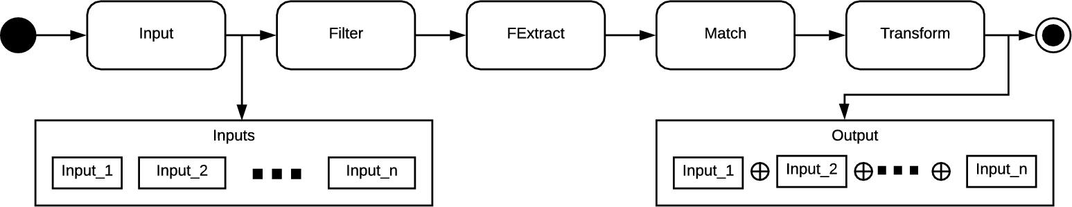
Consider, for example, the following pipeline architecture for a registration system, which is represented in five consecutive states, depicted in Fig. 9.1. This architecture is inspired from the Point Cloud Library (PCL) [8]. From the left, the state Input represents the data acquisition loop which gathers image data from one or more sensors. The second state Filter aims to reduce the data size if necessary so that only the relevant information is used for further processing. In addition, the original images are preserved. The third state FExtract is responsible to compute the predefined key features from the data to reason about the geometric characteristics of the images. The fourth state Match is used to correlate the extracted features with each other. The state Transform is used to transform the original images into a common image based on the matching process. Here, the sign ⊕ represents the transformation operator.
Assume that a version of the PCL library is instantiated in an Ecore MDE environment with the following models which represent the system from different architectural views [9]. More detailed information about these models can be found in Section 9.4.
- • A class model, which describes the logical structure of the system.
- • A feature model, which defines the variations to configure different versions of registration systems.
- • A platform model, which describes the underlying computational resources of the registration system.
- • A process model, which illustrates the execution flow of the processes and the necessary synchronization points among them.
From the perspective of this chapter, the following potential problems can be observed:
- 1. Large configuration spaces of models: It is a common practice that multiple related models are used in MDE environments for a given system. Each of these models may define different kinds of variations. The possible combination of all variations may potentially enable many possible instantiations of models, which can be difficult for the MDE expert to comprehend. Consider, for example, the registration system which is described by four different kinds of models. Due to the variations of each model, the design space of the registration system can be very large. In our example case, for instance, the number of variations of the defined feature model is computed as 6144 (see Section 9.5). There have been a number of proposals, such as model splitting, merging, or transforming [3,4], which can be used to deal with model complexity. However, many of these proposals provide dedicated solutions, for example, through the application of predefined rules.
- 2. Lack of quality concerns in model configurations: This problem is a natural consequence of the previous problem. An important set of criteria for creating a particular configuration from a model space is to select the configuration that fulfills the desired quality attributes.
- For example, while configuring a particular registration system, it may be necessary to check whether the tasks in the process model can be completed on a given platform configuration within a given time. To this aim, it must be possible (i) to decorate the process model with the desired attributes such as the execution times of processes and (ii) to check if the process can be completed on time (schedulability analysis [10]).
- Obviously, new models can be introduced aiming at different architectural views if necessary. Assume that we would like to extend the set of models in the MDE environment with two additional models:
- Energy model: a model to define the energy demanded by processes (also called operations) to complete them on the configuration of the underlying platform in a certain time interval. The factors that affect the completion time of processes depend on the demanded energy by them and the offered energy by the platform configuration.
- Precision model: a model to define the quality of the resulting image accuracy in the registration process. In the implementation, there are alternative algorithmic solutions defined with different precision. Depending on the requirements, a low-precision algorithm may be preferred to a high-precision one for the sake of time performance.
- 3. Optimization of configurations: Software engineers generally have to trade off different quality attributes to configure the most suitable model for a given application setting. For example, a particular model configuration may improve the quality attribute “reducing energy consumption” while decreasing the quality attribute “time performance.” The MDE environment must provide means to optimize model configurations by considering multiple quality attributes.
Based on these observations, it is desired that the OptML Framework must support at least the following requirements.
It must be possible to:
- 1. evaluate configurations of models and whether there exists a configuration that can be mapped on a specified platform architecture while satisfying the time and resource constraints; and/or
- 2. find out the optimal model among configurations based on certain optimization criteria and objectives. Along this line, for example, it must be possible to
- (a) introduce a model for each quality attribute;
- (b) normalize the quality attributes;
- (c) prioritize the quality attributes with respect to each other;
- (d) apply the well-known logical operators on the values of attributes, such as “
 ”;
”; - (e) select the models with respect to minimization or maximization of the quality attributes;
- 3. find out the optimal model among configurations based on certain optimization criteria and objectives; and/or
- 4. find out whether the introduced models are consistent with each other with respect to the predefined consistency rules.
Obviously, software engineers may demand many different kinds of models in developing their applications. The facilities provided by the OptML Framework may need to be extended accordingly. The effort that is spent in realizing the OptML Framework can only be justified if the facilities of the OptML Framework are demanded by multiple software engineers. The OptML Framework, therefore, must offer solutions to the recurring problems of software engineers. If, however, the OptML Framework is required to be extended to satisfy the emerging needs of software engineers, it must be extended accordingly. In addition, enhancements to the implementation of OptML may be necessary from time to time, for instance, to increase performance. Based on these assumptions, the following extensions are considered foreseeable:
- 5. supporting new models defined in the Ecore environment;
- 6. introducing new pruning mechanisms while extracting models from the model base;
- 7. introducing new value-based quality attributes;
- 8. introducing new value optimization algorithms where necessary;
- 9. adopting new search strategies for the schedulability analysis and optimization techniques.
9.3 The architecture of the framework
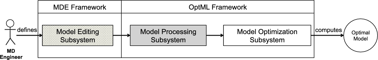
As shown in Fig. 9.2, the architecture of the OptML Framework consists of three subsystems. The Model Editing Subsystem, which is symbolically shown on the left side of the figure, can be used to define various models representing different architectural views based on the corresponding metamodels. If necessary, new metamodels can be introduced to the system using MDE facilities. We assume that this subsystem corresponds to a standard MDE framework such as the Eclipse Modeling Framework. The second process in the figure, the Model Processing Subsystem, is used to transform the introduced models into a representation, which can be processed by the Model Optimization Subsystem. The Model Optimization Subsystem part of the framework, which is shown symbolically at the right-hand side of the figure, automatically processes the transformed models and computes the optimal model based on the criteria provided by the model-driven engineer. The last two processing subsystems form the essential components of the OptML Framework. In our approach, we adopt the Ecore Modeling language and Eclipse Platform for the Model Editing Subsystem. Since this framework is well known, we do not explain it further in this chapter. Nevertheless, in Sections 9.5 and 9.6, we respectively describe the Model Processing Subsystem and Model Optimization Subsystem in detail.
9.4 Examples of models for registration systems based on various architectural views
We will now introduce six models subsequently to illustrate the contributions of this chapter and to deal with the complexity of the example design problem. It is also a common practice in MBSD that a complex design problem is decomposed into a set of models where each represents a different aspect of the system to be designed [11]. Of course, in the end, all the relevant models must be related to each other in some way to represent the system as a whole.
The modeling paradigm adopted in this chapter follows the MDE Ecore tradition, which means that first a metamodel is to be defined that conforms the Ecore metametamodel (called Ecore EMF format) [5]. A model is an instantiation of its metamodel. In the following subsections, the described models are:
- • UML Class model: to depict the logical view [12] of the example;
- • Feature metamodel: to specify the possible configurations of the example [13];
- • Platform metamodel: to specify the physical view and the deployment view [12] of the example;
- • Process metamodel: to specify the process view [12] of the example;
- • Value metamodel: to specify the quality concerns of the example.
These models are selected because they are considered as fundamental models required by many applications as published by Kruchten [12]. In addition, to address the requirements of this chapter, the Value metamodel is introduced so that the optimal model can be computed accordingly.
9.4.1 UML class model
A class diagram is used for specifying the logical building blocks of a software system. We do not define a new metamodel for classes, but rather we adopt the standard UML class metamodel, which is one of the registered packages2 of the Epsilon Modeling Framework in Eclipse IDE.
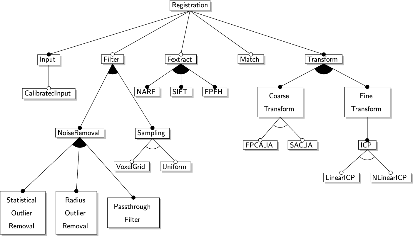
Fig. 9.3 shows a class model for the registration system, which is introduced in Section 9.2. Here, for brevity, the attributes and operations are not shown in the figure.
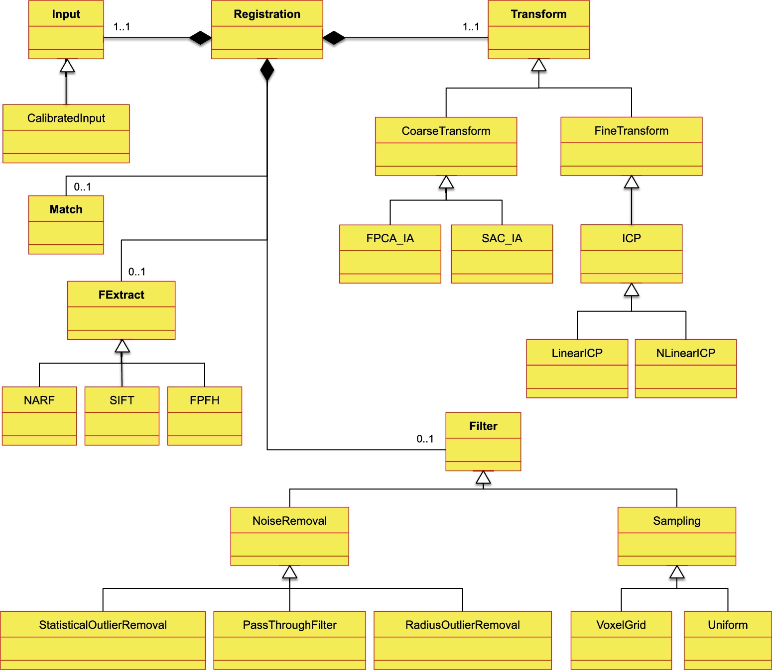
The names of classes Input, Filter, FExtract, Match, and Transform are written bold in the figure, and they correspond to the subsystems of a registration system presented in Fig. 9.1 of Section 9.2.
9.4.2 Feature metamodel
The metamodel representing feature models is shown in Fig. 9.4. The aim of the feature model is to express commonalities and variabilities in a family of software systems. A feature model enables the model-driven engineer to express various configurations of the system. Due to various options, configuring a feature model may result in more than one software system. In the traditional MDE approach, the model-driven engineer is supposed to evaluate each configuration and choose the most suitable one based on some criteria.
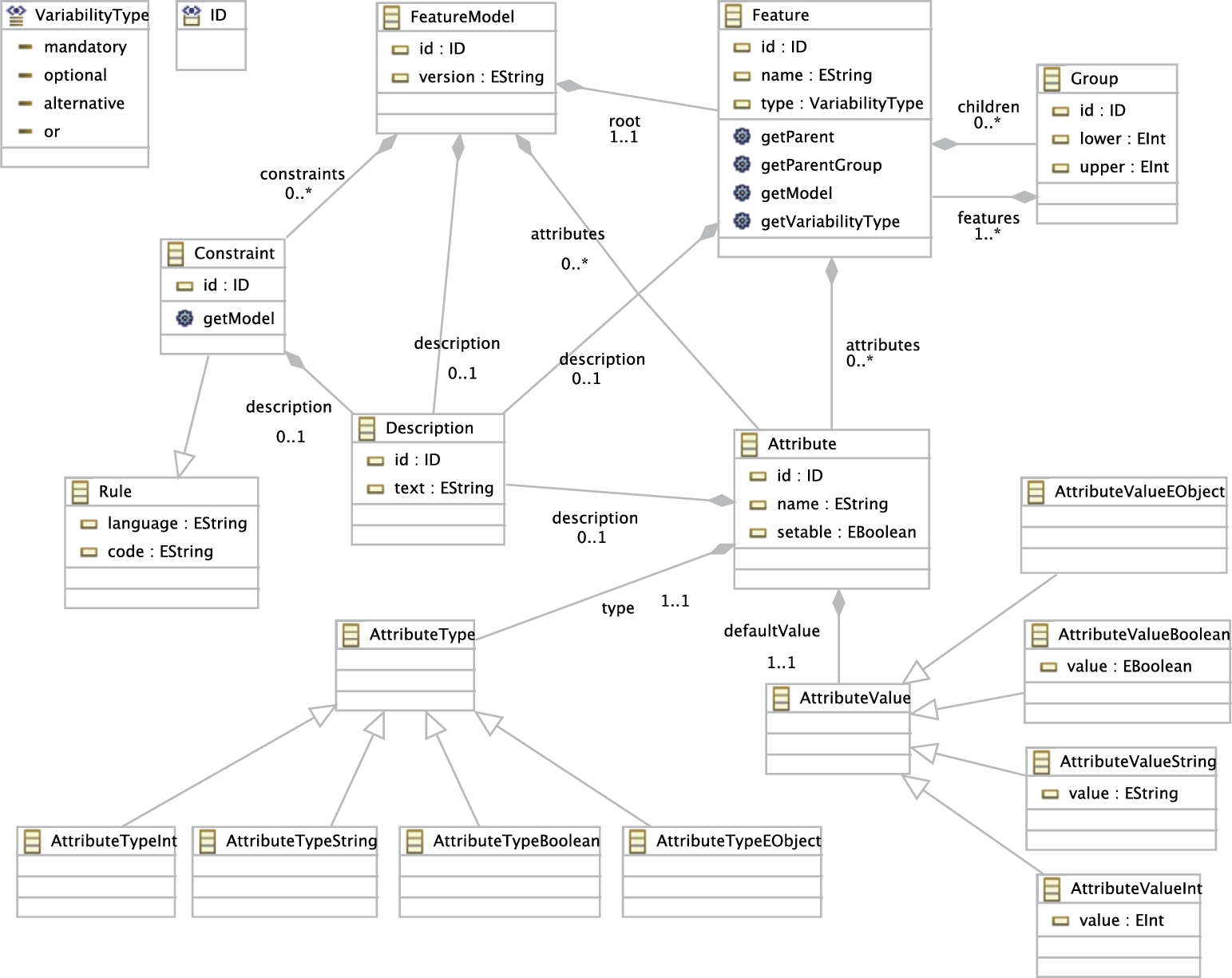
Fundamentally, any feature model has exactly one root from which subfeature models originate. Each feature may have zero or more child features and attributes. Each attribute has a type and defaultValue, which may belong to the types Boolean, String, Integer, or Object. In addition, each feature has a type as optional, alternative, or or if it is a variability; or mandatory if it is a common asset for the product family. All the features are placed into a Group with upper and lower. The number of bound features inside the same group has to be between these values in any configuration instantiated from one feature model. Finally, a feature model may have cross-tree constraints that are defined as rules in any constraint-based language.
A feature model must be consistent with the process model and class diagram. Therefore, we assume that each feature defined in a feature model must correspond to a class in the class diagram.
A feature model of the registration system, which is instantiated from the Feature metamodel, is given in Appendix 9.A.
9.4.3 Platform metamodel
As a third example, we will present the Platform metamodel, as adopted in the OptML Framework. A platform model, which is also termed deployment model [14], is an instance of this metamodel and enables the designer to express the underlying computational system. If a platform model is not specified, it is assumed that the underlying computational system is transparent and as such mapping of software modules to computer architecture is to be handled by the operating system in some way. In many system design problems, however, it may be necessary to take the platform into account, for example, in designing software architecture over distributed and/or multicore systems and in Internet of Things (IoT) applications to map software modules over the underlying architecture.
The Platform metamodel is shown in Fig. 9.5. It expresses hierarchically nested software/hardware architectures, which can be composed of various types of architectural components. The Platform metamodel is represented as class PlatformDiagram, which aggregates classes ResourceType and CompositeResource. The class ResourceType specifies the characteristics of the corresponding resources with a unique string type identifier and an enumeration of the literals active, passive, and composite. We aim to create a uniform model by considering all possible architectures as a special configuration of a composite object. To this aim the class PlatformDiagram aggregates the class CompositeResource. To create a hierarchical platform organization, the class CompositeResource uses the composite pattern format [15]. The class Resource here corresponds to an abstract representation of every architectural component, since every resource inherits its properties. The class CompositeResource may encompass zero or more terminal and/or composite resources, where composite resources may further aggregate resources, and so on. The aggregation relation from the class CompositeResource to the class Resource enables to create nested instances of classes CompositeResource and/or TerminalResource. The class TerminalResource, as the name implies, is the representation of the resources that cannot be decomposed any further. The attribute capacity of the class TerminalResource defines the maximum utilization unit which a resource can provide [16].
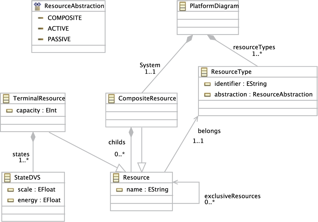
In recent years, mobile devices are increasingly used as a computing platform. Due to limited operational time of batteries, reducing power consumption of mobile devices has become important. To this aim, for example, the Dynamic Voltage and Frequency Scaling (DVFS) technique is introduced [17,18]. In Lin's article [18], the concept of operating frequency levels has been defined. The levels correspond to the frequency scaling factors varying between 0 and 1. A higher value means higher energy consumption. Due to the popularity of this approach in practice, we adopt this technique in our platform model as well; the class StateDVS is introduced for this purpose. Each level has its scaling factor and corresponding power consumption value, which are represented by the attributes scale and energy of the class StateDVS, respectively.
To avoid race conditions and simultaneous access to shared resources, the self-reference relation over the abstract class Resource is defined. It avoids any multiple resources to run at the same time.
The reference relation from Resource to ResourceType is used to denote the type of the corresponding resource.
The platform model as an instantiation of this metamodel for the registration system is given in Appendix 9.B.
9.4.4 Process metamodel
It is considered important to understand the dynamic behavior of systems, for example in allocating software to underlying architecture, verifying the operational semantics of software, or determining the time performance. In the literature, various kinds of models have been presented, such as state diagrams, process diagrams, collaboration diagrams, and activity diagrams. If the time constraints are to be considered in mapping the software system to a particular platform, we assume that a process model is defined which represents the processes and their execution flow, input–output data dependencies, and resource requirements. Consider, for example, the following Process metamodel, which is shown in Fig. 9.6.
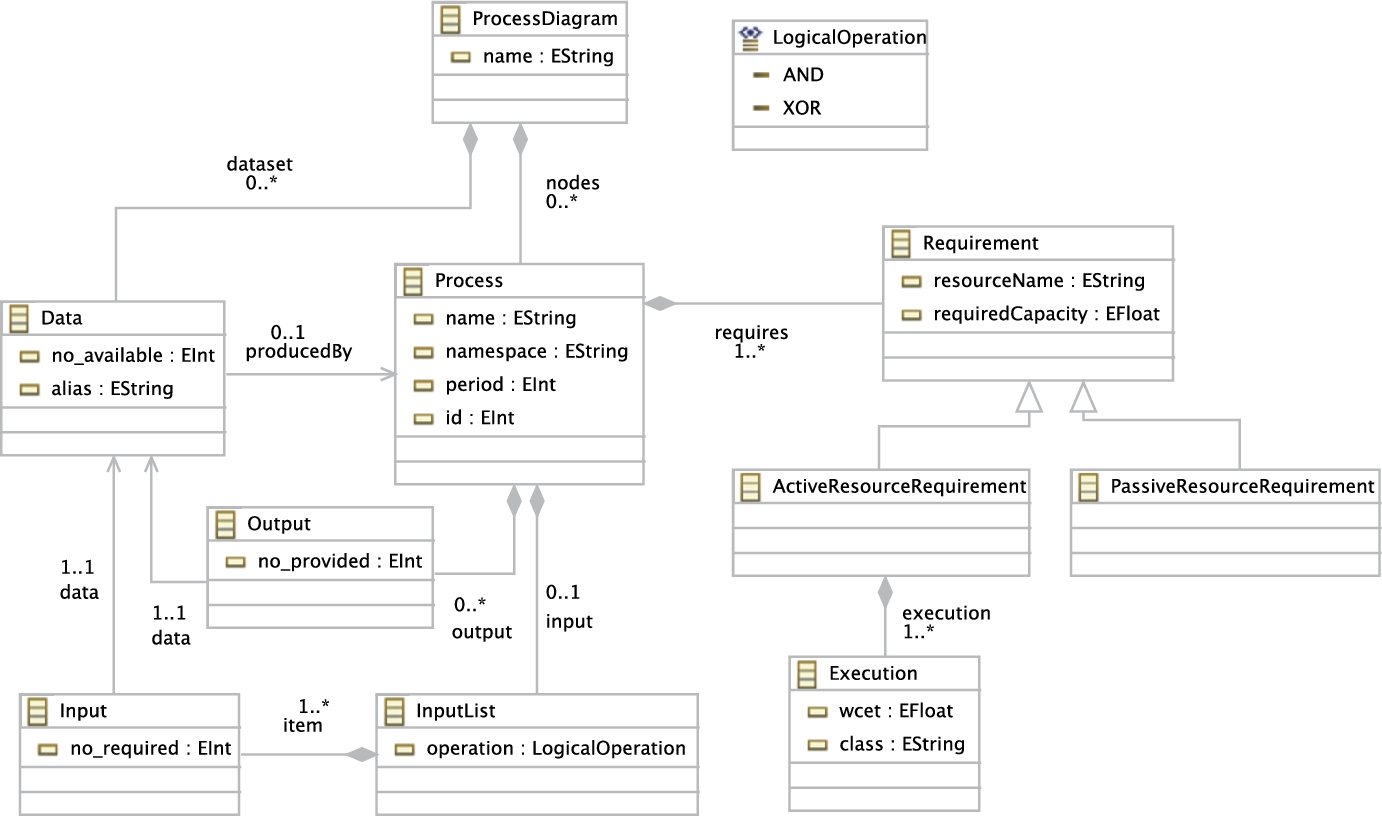
A common practice to represent a process model is to consider it as a graph where each process is a node and the dependencies among processes are the edges of a graph [19]. In our approach, in Fig. 9.6, the class ProcessDiagram represents the root of the graph. Since there may be multiple independent processes in the system, the attribute name of this class is used to denote a particular process diagram.
The class ProcessDiagram aggregates zero or more nodes, where each node is represented by the class Process. The attribute name of this class is used to identify a particular process in a process diagram. In pure object-oriented programs, a process is associated with an object of a class. To represent this property, the attribute namespace is used to denote the corresponding class. In the literature, periodic processes are executed repeatedly at each time interval [20]. To support this characteristic of a process, the attribute period is defined. In case of multiple instances of a process, the attribute id can be used to distinguish the instances from each other.
It may be the case that the application semantics demands a process to be executed in a certain order [20,21]. To specify such conditions, we adopt the data dependency constraint explained in [22,23]. A data dependency constraint specifies the data that are required and/or provided by a process. If, say, the process ![]() provides the data
provides the data ![]() which are demanded by the process
which are demanded by the process ![]() , then
, then ![]() is eligible to be executed only after the completion of
is eligible to be executed only after the completion of ![]() . In the figure, the required and provided data for a process are represented by classes Input and Output, respectively. Both classes refer to only one instance of the class Data. The availability of a particular data item is indicated by the attribute no-available of the class Data. The attributes no-required and no-provided of classes Input and Output refer to the required and provided number of available data items, respectively. The class InputList specifies the input dependency constraints of a process. If a process requires more than one data item and is eligible to start when only one of the data items is available, the attribute operation of the class InputList should be defined as XOR. However, if the process requires the availability of all data items, then the attribute should be defined as AND, instead.
. In the figure, the required and provided data for a process are represented by classes Input and Output, respectively. Both classes refer to only one instance of the class Data. The availability of a particular data item is indicated by the attribute no-available of the class Data. The attributes no-required and no-provided of classes Input and Output refer to the required and provided number of available data items, respectively. The class InputList specifies the input dependency constraints of a process. If a process requires more than one data item and is eligible to start when only one of the data items is available, the attribute operation of the class InputList should be defined as XOR. However, if the process requires the availability of all data items, then the attribute should be defined as AND, instead.
Resource requirements of a process are expressed by the class Requirement. The attributes resourceName and requiredCapacity refer to the necessary resource type and its capacity, respectively. To increase the utilization factor of resources, it may be profitable to divide resource types as active and passive resources [6,24]. To this aim, classes ActiveResourceRequirement and PassiveResourceRequirement are defined, which inherit from the class Requirement. For allocating active resources to processes that complete in a timely manner, worst-case execution time of a process is an important factor to consider. The attribute wcet of the class ActiveResourceRequirement is used for this purpose.
The process model of our example case which is created from the metamodel shown in Fig. 9.6 is presented in Appendix 9.C.
9.4.5 Value metamodel
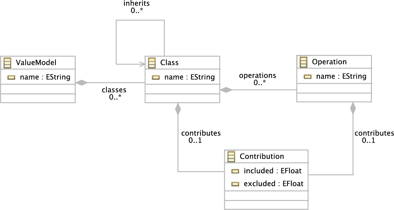
The OptML Framework aims to optimize software models based on various quality attributes. This metamodel assumes that these attributes are expressed in numeric values associated with the models3. If there are multiple attributes, the associated values must be differentiated by the types of the qualities used. We define nevertheless a common Value metamodel, which can be instantiated for different quality attributes if needed. The Value metamodel is shown in Fig. 9.7. Here, the class ValueModel has an attribute name that is used to specify the type of a quality attribute. The value of a quality attribute is assigned to each operation within a class. As a short-hand notation, it is also possible to assign a value to a class. This means however that the values of the operations defined in that class are equal. If two different values are assigned to a class and an operation of that class, the value of the operation overrides the value of the class. It is also possible to override values through inheritance relations. To specify these values, the class Contribution is defined which is associated with Class and Operation. Here, the attributes included and excluded indicate the positive and the negative contribution values depending on the inclusion or exclusion of the corresponding element in the configuration, respectively.
The instantiations of the Value metamodel for energy consumption and computation accuracy are given in Appendix 9.D.
9.5 Model processing subsystem
The Model Processing Subsystem is used to integrate the models with each other. The output of this subsystem is expressed as a dynamic data structure called pipeline data, which will be explained in the following subsections. Fig. 9.8 symbolically depicts the processing steps of this subsystem.
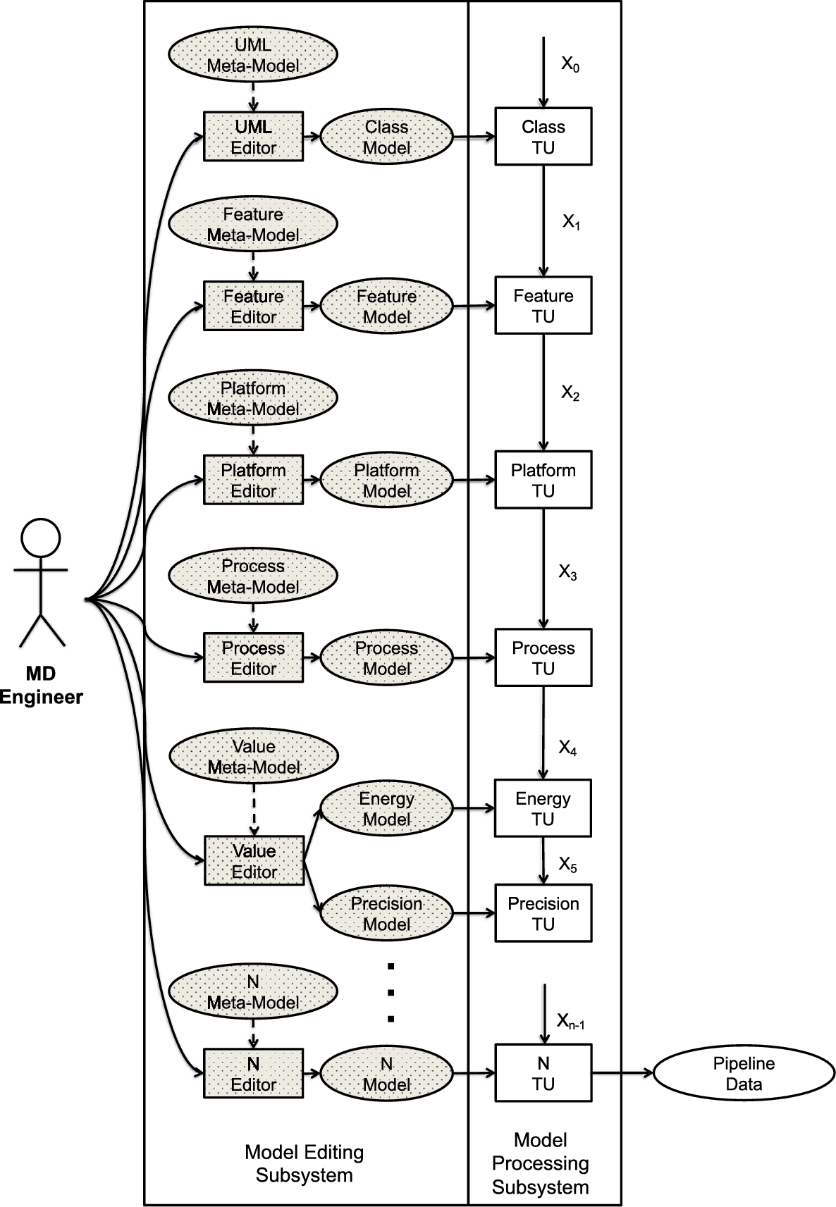
As shown in the figure, for each model that is defined, there exists a corresponding transformation unit (TU). TUs are organized in a pipeline structure and carry out the following two operations: inputModel and transform. The input and output formats of each TU conform to the pipeline data type. The operation inputModel retrieves the corresponding model from the model base.
The operation transform is specialized with respect to the characteristics of the corresponding model. A typical transformation operation consists of the following steps. First, it retrieves the incoming data from the pipeline. Second, it checks the consistency between the incoming data and the corresponding model. An error message is generated in case of inconsistency. Third, it transforms the structure of the corresponding model to the format of the pipeline data. Finally, it concatenates the incoming pipeline data with the transformed data and places it at the output. The next processing unit takes it as an incoming pipeline data, and so on.
An example of pipeline data is represented in Listing 9.1.
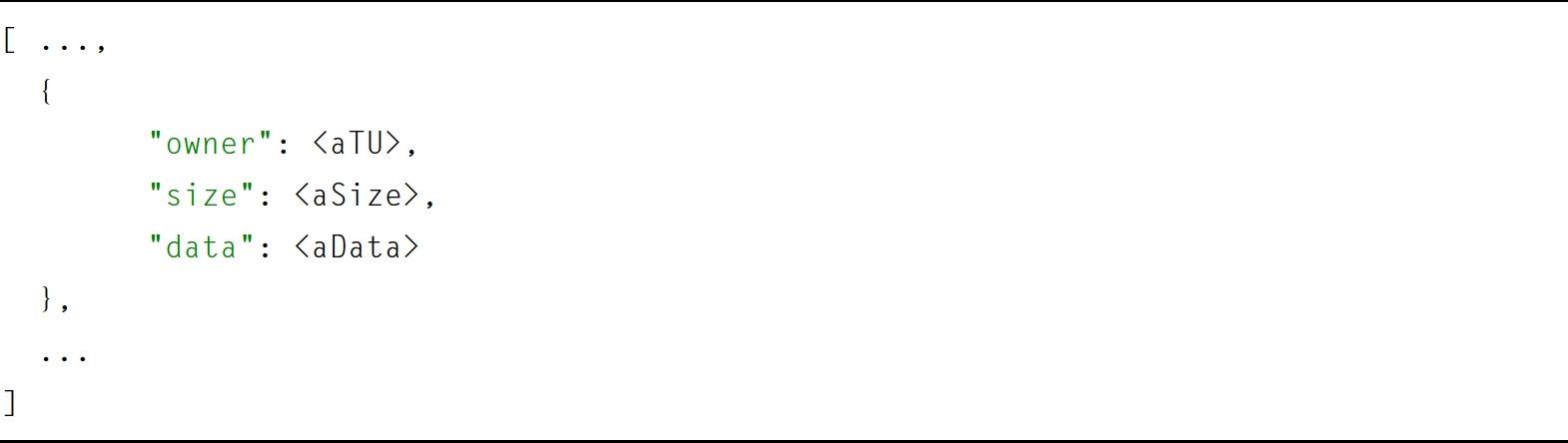
Pipeline data consist of zero or more entities. Each TU adds its own data as an entity to the pipeline data. The three dots before and after the brackets “{” and “}” indicate a possible existence of more entities. The keyword “owner” denotes the identity of the TU which outputs these data. Here, the item “<aTU>” must be replaced with the name of a concrete identity of the corresponding TU. The keyword “size” indicates the number of entries in the corresponding data. The keyword “data” holds the instance of the data type that represents the corresponding model.
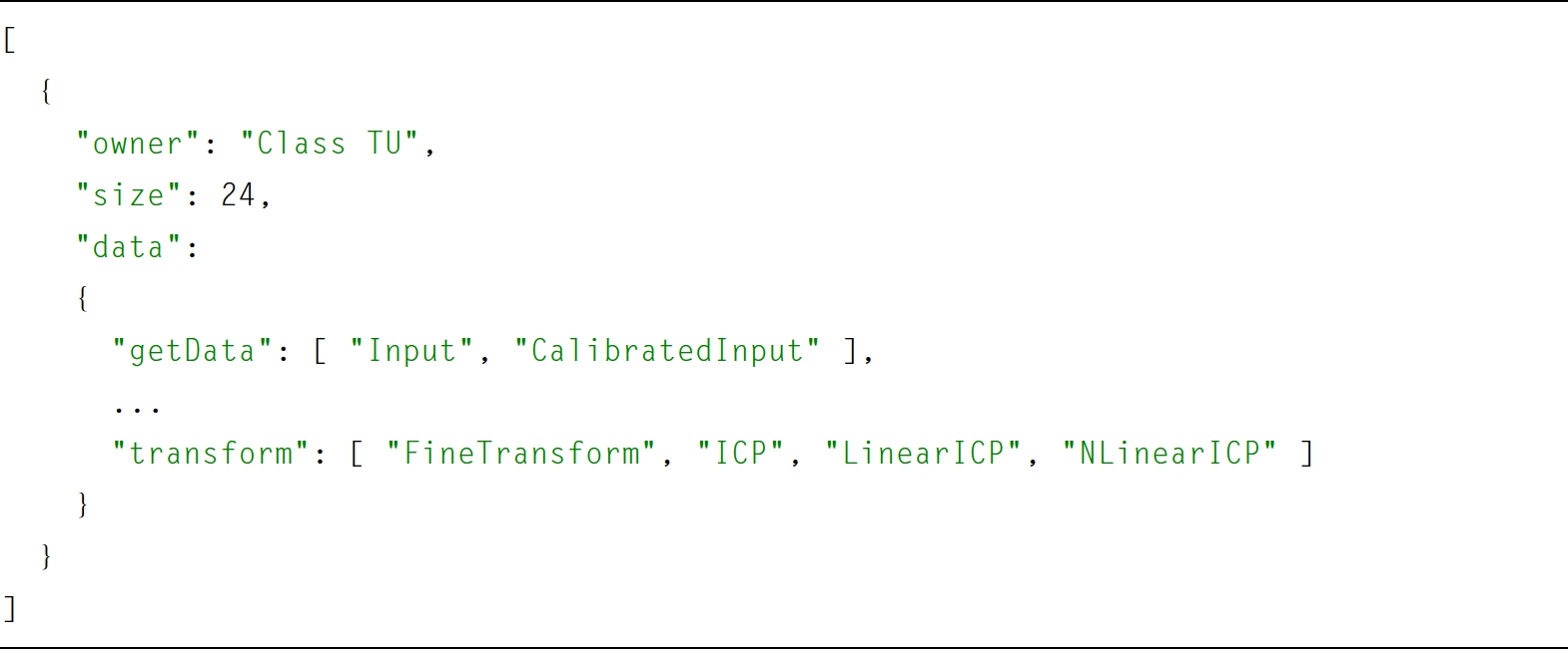
As defined in Fig. 9.8, now assume that the first TU in the pipeline corresponds to a class model. Since this is the first TU in the pipeline, it creates the first entity, which is shown in Listing 9.2. Here, “owner” is defined as “ClassTU,” and the data size is computed as 24. A class model is defined as a “dictionary” where each key indicates an operation and the corresponding value indicates one or more classes that incorporate the operation. This data format is accepted by the Model Optimization Subsystem. In our example class model given in Section 9.4, there are 24 operations with unique names. In the figure, this is represented in the following way. After the keyword “data,” first the operation “getData” and classes “Input” and “CalibratedInput” which incorporate this operation are specified. Following this, 23 more operations must be included in the list. For brevity, in the figure, only the last operation is shown. Here, the operation “transform” is associated with four classes: “FineTransform,” “ICP,” “LinearICP,” and “NLinearICP.”
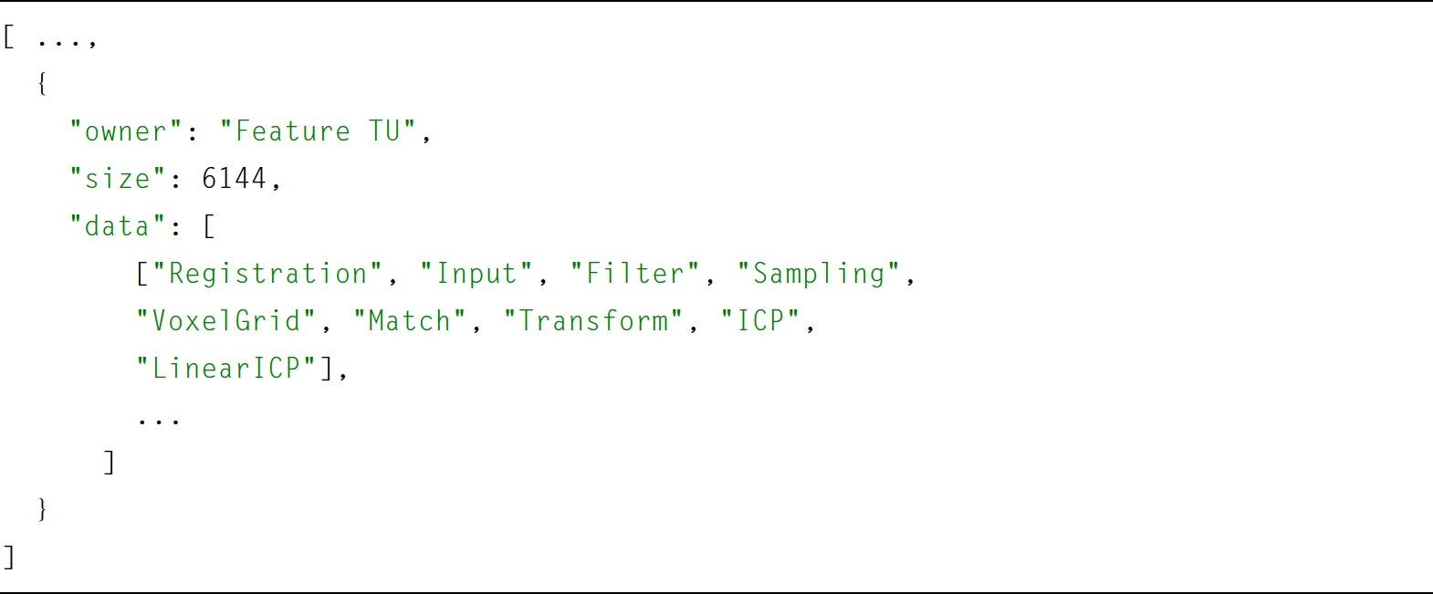
The second TU corresponds to the Feature model. In the description of the feature model, it is assumed that each feature corresponds to a class in the class model. For this reason, Feature TU checks whether for each feature there exists a matching class in the class model. In case of a mismatch, an error condition is raised. In Listing 9.3, the output of our example Feature TU is shown. Here, we will only focus on the keywords “size” and “data.” The value of “size” is calculated as 6144, meaning that with the current specification of the feature model 6144 configurations are possible. Feature TU computes the configurations and adds these as the entries of the instance of the data type list, as required by the Model Optimization Subsystem, and stores it at “data.” For example, the first configuration in the list includes the features “Registration,” “Input,” “Filter,” “Sampling,” “VoxelGrid,” “Match,” “Transform,” “ICP,” and “LinearICP.” For brevity, the remaining configurations are not shown in the figure.
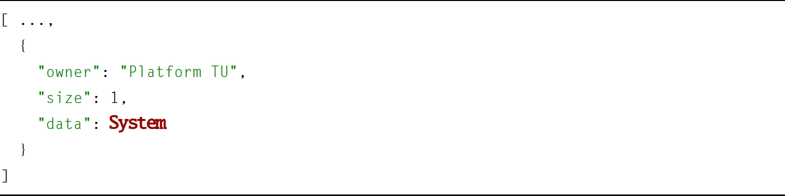
Platform TU is the third unit in the pipeline. The output of this TU is shown in Listing 9.4. The keyword “size” is set to value one, meaning that there is only a single entry in the model and that is the platform model. The keyword “data” refers to the instance object of the platform model, denoted by the variable name System, which is defined in the model base. The Model Optimization Subsystem directly accepts the models (objects) that conform to the Platform metamodel.
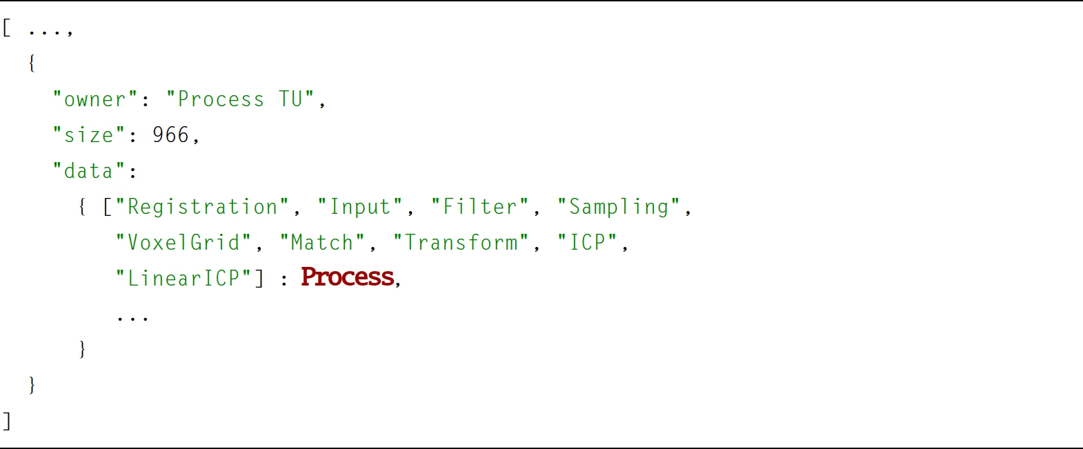
Process TU is defined as the fourth unit in the pipeline. In the process model, it is assumed that each process corresponds to an operation in the class model. Furthermore, there exists a consistency relation between the process model and the feature model, since there exists a one-to-one relation between features and classes. Therefore, Process TU first checks whether these conditions are satisfied. It is possible that while configuring the Feature model some of the optional features are not included. The operations corresponding to these excluded features must be excluded from the process model as well. Listing 9.5 shows the output data of Process TU. From the figure, it can be seen that the value of “size” drops from 6144 to 966 due to the elimination of the irrelevant configurations in our example. The data are organized as a dictionary type where the keys are the configurations and the values are the corresponding instances that represent the relevant portions of the process model. The Model Optimization Subsystem requires this dictionary data type. In Listing 9.5, only the first entry of the dictionary is shown. Here, the features “Registration,” “Input,” “Filter,” “Sampling,” “VoxelGrid,” “Match,” “Transform,” “ICP,” and “LinearICP” correspond to a relevant configuration of the feature model. This configuration is associated with the instance Process that includes the portion of the corresponding processes. In the figure, for brevity, the remaining 965 instances are not shown.
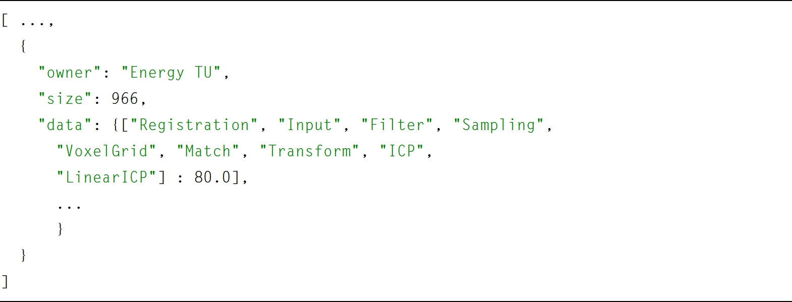
Energy TU is defined as the fifth unit in the pipeline. As the first step, Energy TU checks if the Energy model and the models retrieved from the pipeline data are consistent with each other. In this context, the consistency is specified as follows. Every class and operation defined in the Energy model must conform to the class model. Second, the configurations of processes are taken from the pipeline data and the total energy value per configuration is computed. Third, Energy TU creates a dictionary where the keys are the relevant configurations, and the values are the total energy value of the processes that are utilized in the corresponding configuration. Finally, this dictionary is concatenated with the incoming pipeline data and placed at the output. This data representation is required by the Model Optimization Subsystem. An example of output pipeline data is shown in Listing 9.6. Consider now the keyword “data.” Here, only the first configuration is shown, which consists of “Registration,” “Input,” “Filter,” “Sampling,” “VoxelGrid,” “Match,” “Transform,” “ICP,” and “LinearICP.” In this example, the total energy value consumed by this configuration is computed as 80.0.
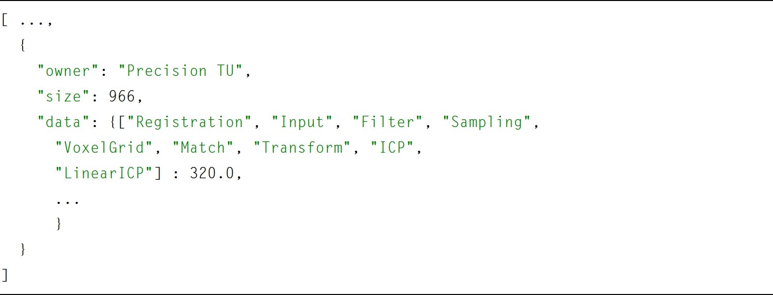
The last unit in the pipeline is Precision TU. The steps carried out in this TU are the same as in the previous one, namely, checking consistency, extracting configurations from the process model, computing the value of each configuration, and concatenating the obtained data with the incoming pipeline data. Of course, in this context, the values correspond to the precision values. The output pipeline data are shown in Listing 9.7. The first configuration associated with“data” is the same but the associated value of this configuration is computed as 320.0.
9.6 Model optimization subsystem
In this section, we first define the adopted optimization process. Second, we shortly describe the architecture of the subsystem. Finally, we give three example scenarios to illustrate how the subsystem computes the optimal model according to the given constraints.
9.6.1 Definition of the optimization process
The OptML Framework is used to optimize software models. According to our definition, the essential property of every software system is the execution of operations according to a certain program. The Process metamodel is defined to express the dynamic behavior of a software system. The model-driven engineer must specialize this metamodel to describe the dynamic behavior of the system being designed. This model is particularly useful to compute the timeliness and energy consumption properties of the models.
A process configuration corresponds to a program which is defined as a valid set of processes conforming to its process model. In general, more than one process configuration can be derived from a Process model. We assume that if there are inconsistent models, they are detected by the Model Processing Subsystem before the pipeline data reach the Model Optimization Subsystem.
The Model Optimization Subsystem searches for a solution of a process configuration where each process is allocated to the appropriate elements of the Platform model, while satisfying the constraints4 defined by the model-driven engineer of each process. Currently, the following constraints are supported:
- • The capacity. This is specified based on the units of the relevant platform elements. Examples are memory size and processing power.
- • The worst-case execution time.
- • The release time.
- • The deadline.
- • The dependency constraints.
- • The preemption constraint.
- • The migration constraint.
- • The mutual-exclusion constraint.
The Platform model specifies the resources and their characteristics so that they can be matched to the constraint embedded in the process model.
While searching for an optimal configuration, the Model Optimization Subsystem may adopt various strategies among the set of candidate configurations, such as first-fit, nth-fit, and first-n searches. In the first-fit search approach, the first configuration that satisfies the requirements is selected and the search process is terminated. In the nth-fit search, as the name implies, the first n valid configurations are selected if existing. Finally, in the first-n search, the first n configurations are selected even if some of them are invalid.
In additional to the process requirements, the optimization process can be extended by defining constraints which can be derived from the Value metamodel, similar to the examples of the energy and precision models presented in Appendix 9.D. These additional constraints are only meaningful if more than one configuration is considered. The configurations that satisfy the process requirements and are within the boundaries of the desired value constraints are ranked according to the optimal required value. The optimal value may be either a minimum or a maximum of the values of the considered configurations.
A Class model is a static representation of a program, and as such it defines the bindings of processes to the operations of classes which can be overridden through inheritance. Therefore, the class model restricts the definition of configurations derived from the Process metamodel. Similarly, the Feature model can be seen as a restriction over the Class model.
9.6.2 The architecture of the model optimization subsystem
The Model Optimization Subsystem consists of three components: Adapter, Value Processor, and Schedulability Analyzer, as shown in Fig. 9.9.
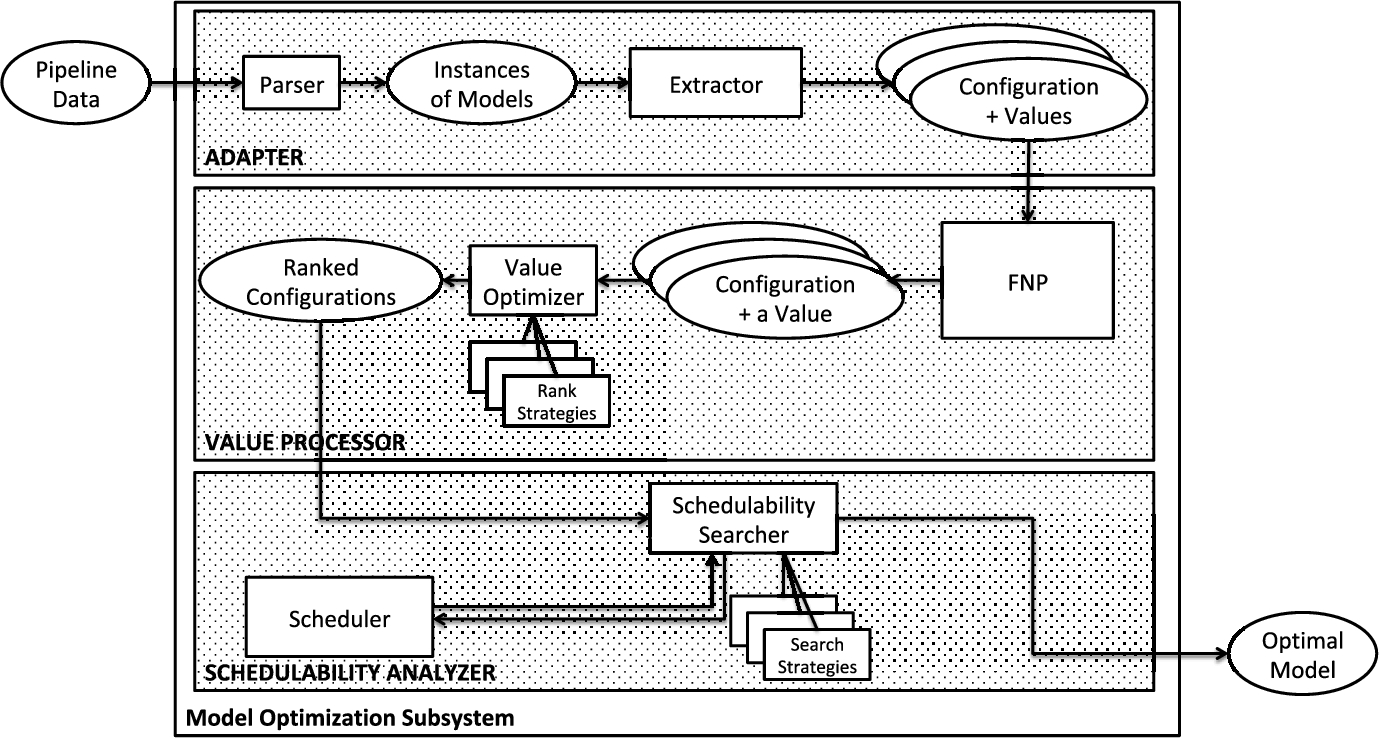
Adapter has two subcomponents:
- • Parser accepts the pipeline data as input and extracts the instances of models that are generated by the transformation units. These are a dictionary representing the class model, a list of configurations obtained from the feature model, an instance object that represents the platform, a dictionary of process configurations, and two dictionaries representing energy and precision models, respectively.
- • Extractor processes the instances of models and generates a list of process configurations associated with the values to be considered for the optimization process.
The module Value Processor includes two subcomponents:
- • FNP implements three operations, i.e., Filter, Normalize, and Prioritize. The operation Filter eliminates the process configurations which have associated values out of the desired boundaries. For example, the model-driven engineer may indicate that the precision value must be above a certain number and/or the energy value must be less than a certain number. Second, the operation FNP normalizes each value between 0 and 1. Finally, based on the input given by the model-driven engineer, the operation Prioritize computes a single value using the following formula:
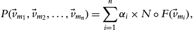
- where
 represents the priority of the corresponding model
  to the total equation,
  indicates the composition of functions normalize and filter, and
  represents the list of values of the process configurations computed according to the value model .
 - • Value Optimizer ranks the list with respect to the selected Rank Strategy in an ascending or a descending order. According to the choice of the strategy, the model-driven engineer may request for the best n process configurations rather than delegating all of them to the following subcomponent Schedulability Searcher. The best configurations are computed by using an appropriate optimization algorithm. In this way, only the most promising configurations are considered first. If no quality attributes are defined, this component has no effect.
The module Schedulability Analyzer incorporates two subcomponents:
- • Scheduler is based on an application framework called First Scheduling Framework (FSF) [26], which provides the necessary abstractions and mechanisms to implement schedulers. Currently, this framework supports the following abstractions as class hierarchies: Tasks, Resources, Scheduling characteristics, and Scheduling Strategy. The task and resource models of FSF are of the same type as the process and platform models of the OptML Framework, respectively. Upon defining a scheduling application using the provided models, the scheduling constraints are translated to the mathematical constraints to be solved in the generic constraint solvers provided by FSF. Since the models defined in this chapter are designed in accordance with the models in FSF, the transformation of the models is realized in the following way. Firstly, the platform model in OptML is translated to the resource model in FSF. Secondly, the Process model that defines the execution flow of the operations in the Class model is converted to the task model in FSF. Thirdly, the scheduling characteristics are defined with respect to the requirements of each process defined in Section 9.6.1, and scheduling strategy is defined as minimizing the makespan. Since the execution time of a process in the Process model changes with respect to the class in which it is defined, a separate scheduling problem is generated for each configuration. In the sense of schedulability, any feasible solution (schedule) computed by Scheduler makes the corresponding process configuration valid.
- • Schedulability Searcher implements the search algorithm based on a certain strategy. To this aim, it retrieves the top element of the ranked configurations from the subcomponent Value Processor and calls on Scheduler to evaluate it. Depending on the result of this evaluation this process may iterate over the remaining configurations in the ranked list based on the selected strategy. For example, if the first-fit strategy is used, Schedulability Searcher terminates the search as soon as Scheduler finds a solution that satisfies the constraints. This configuration is considered to be the optimal model. Other related models such as the Class model can be reconstructed based on this result.
9.6.3 Example scenarios
In the following subsections, we will give a set of model optimization scenarios to illustrate the utility of the OptML Framework with respect to the requirements defined in Section 9.2. In practice, it is not possible to validate the correctness of a software system with the help of user-defined scenarios since the number of scenarios in any practical system can be extremely large. Therefore, we categorize the scenarios in the following way: (i) time analysis on a single- and multiprocessor architecture; (ii) model optimization based on time analysis combined with a single quality attribute; (iii) model optimization based on time analysis on multiple quality attributes; and (iv) three different search strategies to find an optimal model. We assume that these four categories represent a large number of scenarios that can be experienced in practice.
With respect to the requirements given in Section 9.2, the fulfillment of the first three requirements, finding the schedulable optimal model while satisfying the quality requirements, is demonstrated by the three categories of the scenarios that will be given in the following subsections.
9.6.3.1 Scenario 1: finding out the schedulability of the model with respect to a platform model
This scenario aims at justifying the fulfillment of the first requirement: schedulability of processes on platforms. To this aim, we have made the following assumptions about the models:
- • The class, feature and process models are taken from the appendix.
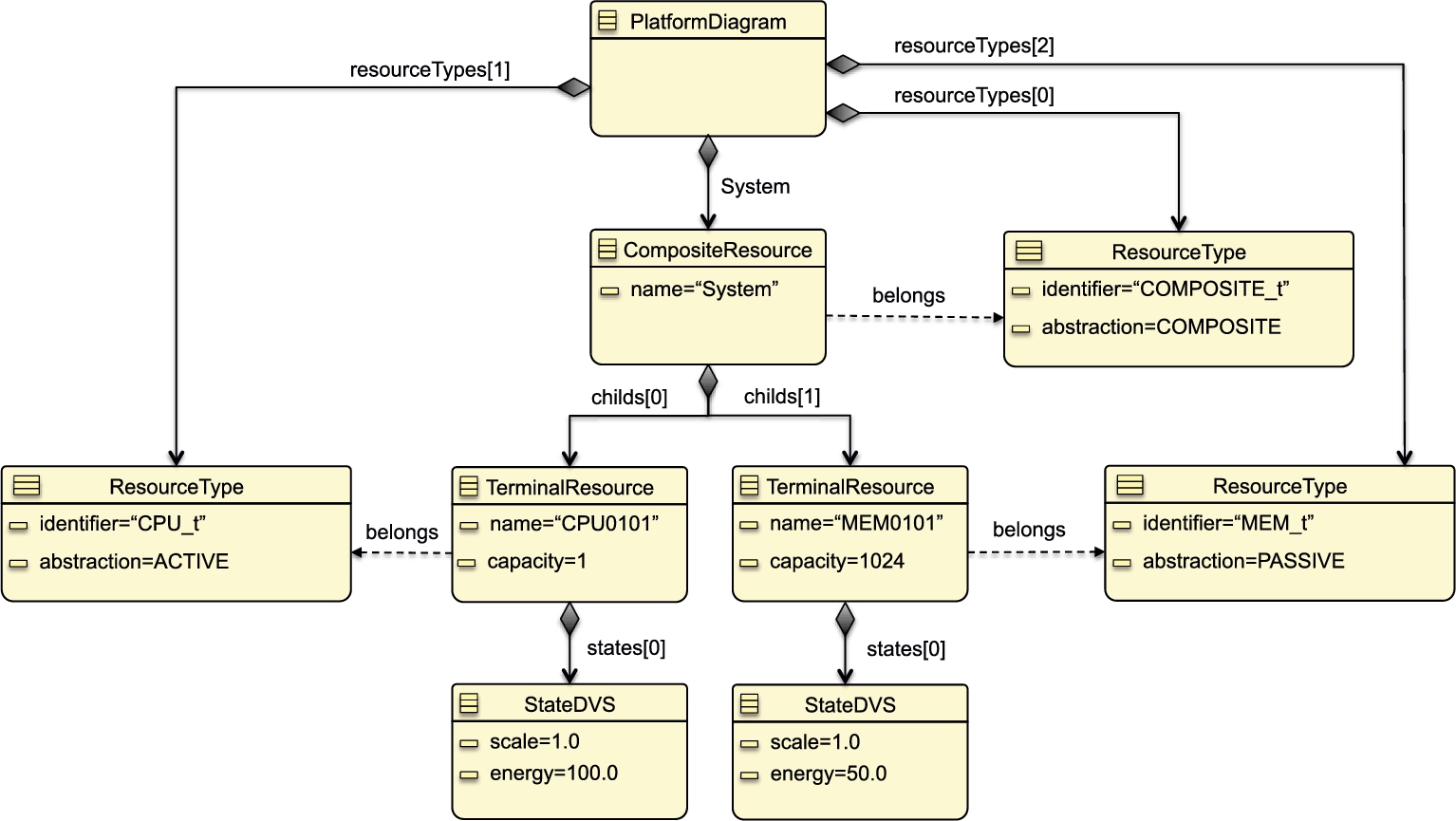
- • The platform model has the following characteristics: It has two terminal resources cpu0101 and mem0101, belonging to active and passive resource types, respectively. The object diagram for the corresponding platform model is shown in Fig. 9.10. The capacity of the active terminal resource is 1; the passive terminal resource has 1024-unit capacity. Each of these terminal resources has one running state. In this scenario, we choose a platform model with single processing unit that is more restricted than the one given in the appendix to demonstrate the effect of platform capacities on the schedulability process.
- • The criteria of the scheduling objective is set to “minimizing the maximum makespan” [21].
- • The scheduling window for the processes is set to 50.
- • The search strategy is chosen as first-fit.
- • The process configurations are not ranked by the subcomponent Value Optimizer.
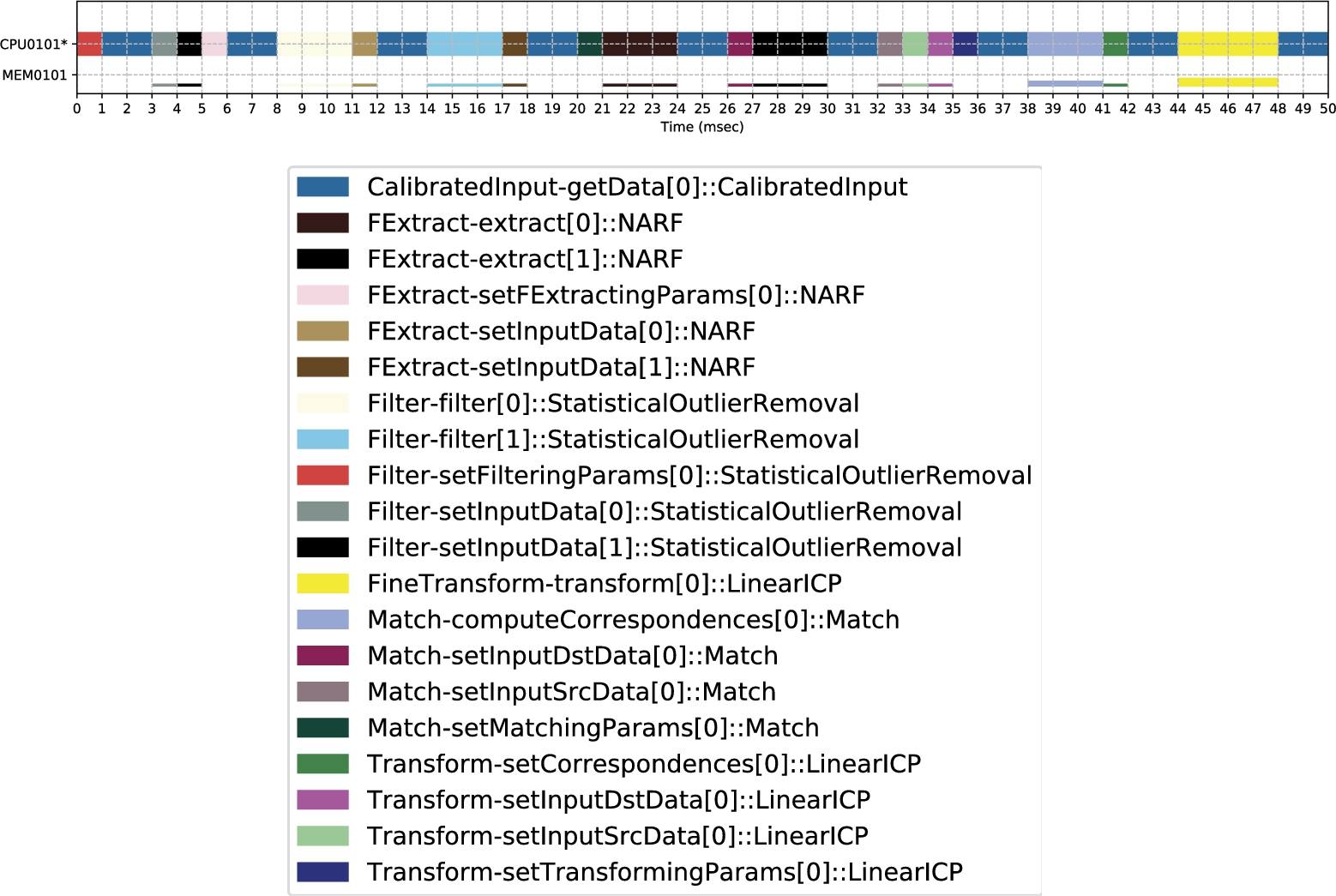
With these given assumptions, Scheduler returns a solution that is depicted in Fig. 9.11. The figure consists of two rectangles. The top horizontal rectangle depicts the schedule computed by Scheduler. This figure only includes the processes that are selected by the optimizer. The horizontal axis corresponds to Time, and the vertical axis corresponds to the capacities of the two terminal resources, cpu0101 and mem0101. Each unit in the vertical coordinate corresponds to total amount of capacity for each resource. The larger rectangle shows all processes, some of which may not be included in the schedule. The legend of each process is indicated by a different color.
9.6.3.2 Scenario 2: finding the schedulable optimal model with respect to a single quality attribute
The second scenario is defined to illustrate the first three requirements in Section 9.2: introducing new quality attributes and finding out the optimal model that satisfies both the schedulability and the quality requirements.
Along this line, the following assumptions are made:
- • The class, feature, platform, and process models are taken from the appendix.
- • A single quality model energy consumption is introduced, which is defined in the appendix.
- • The criteria of the scheduling objective is set to “minimizing the maximum makespan.”
- • The scheduling window for the processes is set to 23.
- • The search strategy is chosen as third-fit.
- • The process configurations are ranked by the subcomponent Value Optimizer with respect to the ascending energy values.
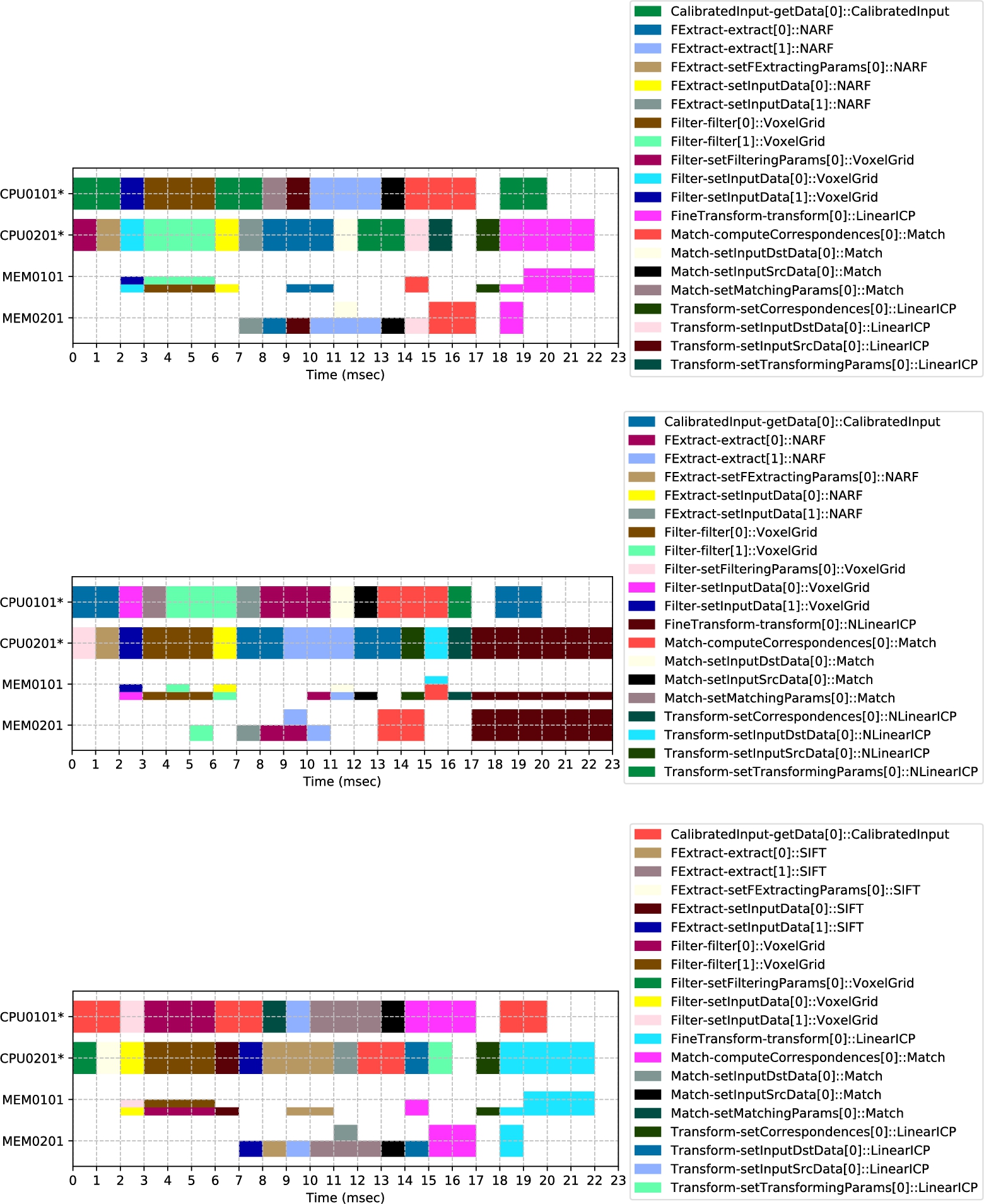
In this scenario, the multiprocessor architecture is selected. The result of the optimization process based on the given assumptions is shown in Fig. 9.12. This figure consists of three subfigures, where each subfigure shows the evaluation of a particular process configuration. The top subfigure shows a schedule with the lowest energy consumption; the bottom subfigure shows one with the highest consumption among the ones that are evaluated. Therefore, the top subfigure is considered as the optimal model.
9.6.3.3 Scenario 3: finding the schedulable optimal model with respect to multiple quality attributes
This scenario extends the previous one with an additional quality attribute precision. To this aim, the assumptions are the same as the previous scenario, except the following:
- • The scheduling window size is set to 21.
- • The search strategy is set to first-25.
- • A new quality attribute precision is defined in the appendix.
- • The priorities of the quality attributes energy and precision are defined as 0.2 and 0.8, respectively.
- • The process configurations are ranked by the subcomponent Value Optimizer with respect to the ascending energy and precision values. To preserve uniformity, a normalized value of 1 corresponds to lowest precision, whereas 0 is the highest.
The result is presented in Fig. 9.13. Here only two configurations are shown. The second configuration found in the ranked configurations happens to be not schedulable, because the operation transform exceeds the specified scheduling window size if it is implemented with a high precision value.
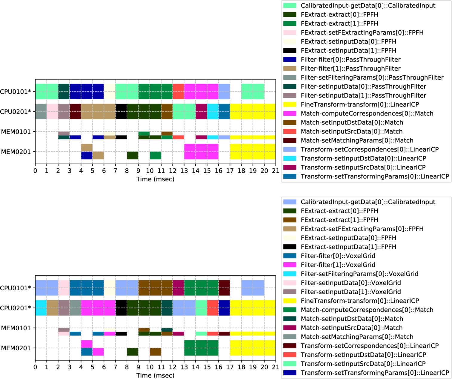
The figure consists of two subfigures, where the top subfigure corresponds to a configuration with a higher quality value. This configuration is selected as the optimal model.
9.7 Related work
Model-Driven Architecture (MDA) aims at separating platform-independent and platform-dependent models from each other [28]. MDE extends MDA with metamodels and model transformations [29]. In MDE, not only models but also metamodels and model transformations are the core assets of software development. The research activities in MDE are very broad, including domain-specific models, model building, model verification, model reuse, model transformation, and code generation [30,31].
In the literature, the terms model and optimization are used in two ways: (i) models for optimization and (ii) model optimization. There have been considerable works on models for optimization where researchers investigate mostly mathematical models to define and implement optimization processes. For our approach, such techniques are adopted in the subcomponents FNP and Value Optimizer for value optimization and in the subcomponents Schedulability Searcher and Scheduler for schedulability analysis.
The purpose of model optimization, however, is to search for the models within a model base that satisfy certain criteria. This is the main focus of the chapter. In contrast to models for optimization, there are hardly any publications that address this problem. As stated by Chenouard [32], a constraint programming-based design synthesis process is presented using MDE techniques. A similar approach is adopted in Joachim's article [33], where an optimal model is searched within the context of certain requirements. The difference between these two articles is that in the former, the optimal model is searched at a model level using constraint programming, whereas in the latter, search is defined as a model transformation. The objectives of both articles are, however, different than ours. The aim in these articles is to synthesize the optimal model which satisfies the constraints, whereas in our work, the aim is to select the optimal model among model configurations which satisfies the constraints. There are a number of research works which aim at verifying models based on certain specifications. With the help of OCL [34], for example, certain properties of models can be formally specified. Also various tools have been developed to verify models decorated with such specifications [35]. These tools in general are used for verification and testing purposes but not for model optimization.
To the best of our knowledge, there is no framework proposal that aims at optimizing models defined in the context of MDE, as proposed in this chapter.
There has been a number of research works aiming at optimizing software architectures according to a set of quality attributes. In [36], algorithms are proposed to optimize TV architectures for the qualities availability, reduced memory usage, and time performance. Multiobjective optimization techniques are proposed in [37] with respect to certain quality attributes such as production speed, reduced energy usage, and print quality. A design method for balancing quality attributes energy reduction and modularity of software is proposed in [38].
9.8 Evaluation
We will now evaluate this chapter with respect to the nine requirements given in Section 9.2. The fulfillment of the first three requirements given in Section 9.2 is explained in Section 9.6.3.
The fourth requirement, checking consistency among models, is realized by the TUs defined in the Model Processing Subsystem, as explained in Section 9.5.
The fifth requirement, supporting new models in the Ecore environment, is provided with the following condition: For each new model, the tool engineer must define the corresponding TU with the necessary model extraction, consistency checking, and model transformation functions.
The sixth requirement, pruning models, is supported in the TUs by redefining the operation inputModel with different retrieval strategies so that only the relevant parts of the model are selected. For example, in the current implementation of the framework, we support the following strategies: (a) retrieve the complete model (default); (b) include only the classes denoted by the model-driven engineer; and (c) include all the classes with a query. The architecture allows introducing new strategies modularly. However, if not all model elements are selected, the pruned model can be inconsistent with the other models. In our framework, for example, if some classes, which are eliminated from the class model, are included in the feature model, the feature TU will give an error message. For brevity, this chapter does not focus on the pruning techniques. An interested reader may refer to the following report [39]. As explained in Section 9.5, due to the pipeline architecture of the Model Processing Subsystem, the framework allows the tool designer to introduce such extensions to the existing utilities.
As demonstrated in Section 9.6.3, the seventh requirement, introducing new quality attributes, can be realized by specializing the Value metamodel with the following restrictions: (a) the quality attributes are expressed in numbers and associated with classes and their operations; and (b) if necessary, the quality attributes per configuration are computed by the corresponding TU. If this way of representing the desired quality attribute is not appropriate, a new Value metamodel and the corresponding TU must be introduced. The pipeline architecture of the Model Processing Subsystem makes this possible without changing the other TUs.
The eighth requirement, introducing new value optimization algorithms, is supported in the following way: Currently, the OptML Framework implements a rather straightforward value optimization based on filtering, normalizing, prioritizing, and priority-based ranking with the help of the subcomponents FNP and Value Optimizer. Different quality values are merged into a single value. As the next step, the schedulability of the ranked configurations is analyzed. One may adopt, however, different value optimization techniques depending on the needs, and the feasibility of time and space complexity of the optimization algorithms. For example, one may aim at reducing the time of optimization processes by using heuristic rules. In the literature, various optimization algorithms are presented, such as hill climbing, exhaustive search, and pareto-front multiobjective optimization [36]. These changes can be encapsulated in the subcomponents FNP and Value Optimizer.
The last requirement, adopting new search strategies for scheduling, can be introduced by defining a new search strategy for the subcomponent Schedulability Searcher.
The time performance of the model optimization process is considered important for the usability of the framework. The current architecture allows performance improvement in the following ways: (a) introducing effective model pruning strategies in the corresponding TUs; (b) applying different optimization algorithms in the Model Optimization Subsystem; (c) using efficient schedulability search strategies; and (d) using efficient solvers in the subcomponent Scheduler.
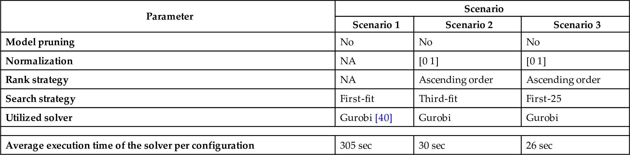
The average execution times of the solver per configuration are shown in Table 9.1. In the figure, the bottom row shows the results of the evaluation. The top five rows define the parameters of the implementations. In none of these scenarios, model pruning is used. Normalization of the quality values is only applied to the second and third scenarios where the values are mapped into the range of 0 to 1. Here, NA means not applicable. The definitions of rank and search strategies are self-explanatory. The row “Utilized solver” defines the constraint solver that is used in the subcomponent Scheduler. The execution time of the solver for Scenario 1 is much higher due to the longer schedulability window size. The time that is required to search among the possible solutions by the subcomponent Schedulability Searcher is negligible when compared with the time performance of the solvers. Of course, to determine the total time performance, one needs to multiply the last column value with the number of iterations in the search strategy.
Table 9.1
The performance values of the scenarios. The scenarios are implemented on a MacBook Pro with 2.6 GHz Intel Core i5 processor and 8 GB 1600 MHz memory.
| Parameter | Scenario | ||
|---|---|---|---|
| Scenario 1 | Scenario 2 | Scenario 3 | |
| Model pruning | No | No | No |
| Normalization | NA | [0 1] | [0 1] |
| Rank strategy | NA | Ascending order | Ascending order |
| Search strategy | First-fit | Third-fit | First-25 |
| Utilized solver | Gurobi [40] | Gurobi | Gurobi |
| Average execution time of the solver per configuration | 305 sec | 30 sec | 26 sec |
9.9 Conclusion
This chapter identifies the following problems: (a) model complexity; (b) the lack of quality-based model selection; and (c) the lack of support of multiple quality-based evaluations. To address these problems, the OptML Framework is presented. This framework accepts various models defined in the Ecore MDE environment, processes them according to user preferences and model properties, and computes the optimal schedulable models based on value optimization and constraint-based scheduling algorithms. To the best of our knowledge, this is the first generic MDE framework that is suitable for model optimization.
The utility of the framework is demonstrated by implementing three scenarios inspired from registration systems used in the area of image processing. The scenarios show that the required objectives of model optimization as defined in this chapter are fulfilled. With the help of design patterns and various architectural styles, the architecture has a modular structure and thereby allows for the introduction of new strategies for model extraction and transformation, value optimization, and schedulability analysis. The framework is fully implemented and tested. It integrates a number of third-party software such as Eclipse EMF [41], pyecore [42], pyuml2 [43], FSF [26], Numberjack [44], matplotlib [45], Gurobi [40], SCIP [46], and Mistral [47].
Appendix 9.A Feature model
The tool designer instantiates the Feature metamodel shown in Fig. 9.4. The instantiated model is shown in Fig. 9.14. The number of systems that can be configured from this model is computed as 1288.
In this section, we present a feature model for the example registration system. This model conforms to the Feature metamodel presented in Fig. 9.4 of Section 9.4. This model is used in the scenario implementations presented in Section 9.6.3. By definition, in our framework, each feature corresponds to a class in the class model. The descriptions of the names of the adopted features are presented in Section 9.4.2. To avoid repetition, the features are not described here again. The number of systems that can be configured from this model is computed as 1288.
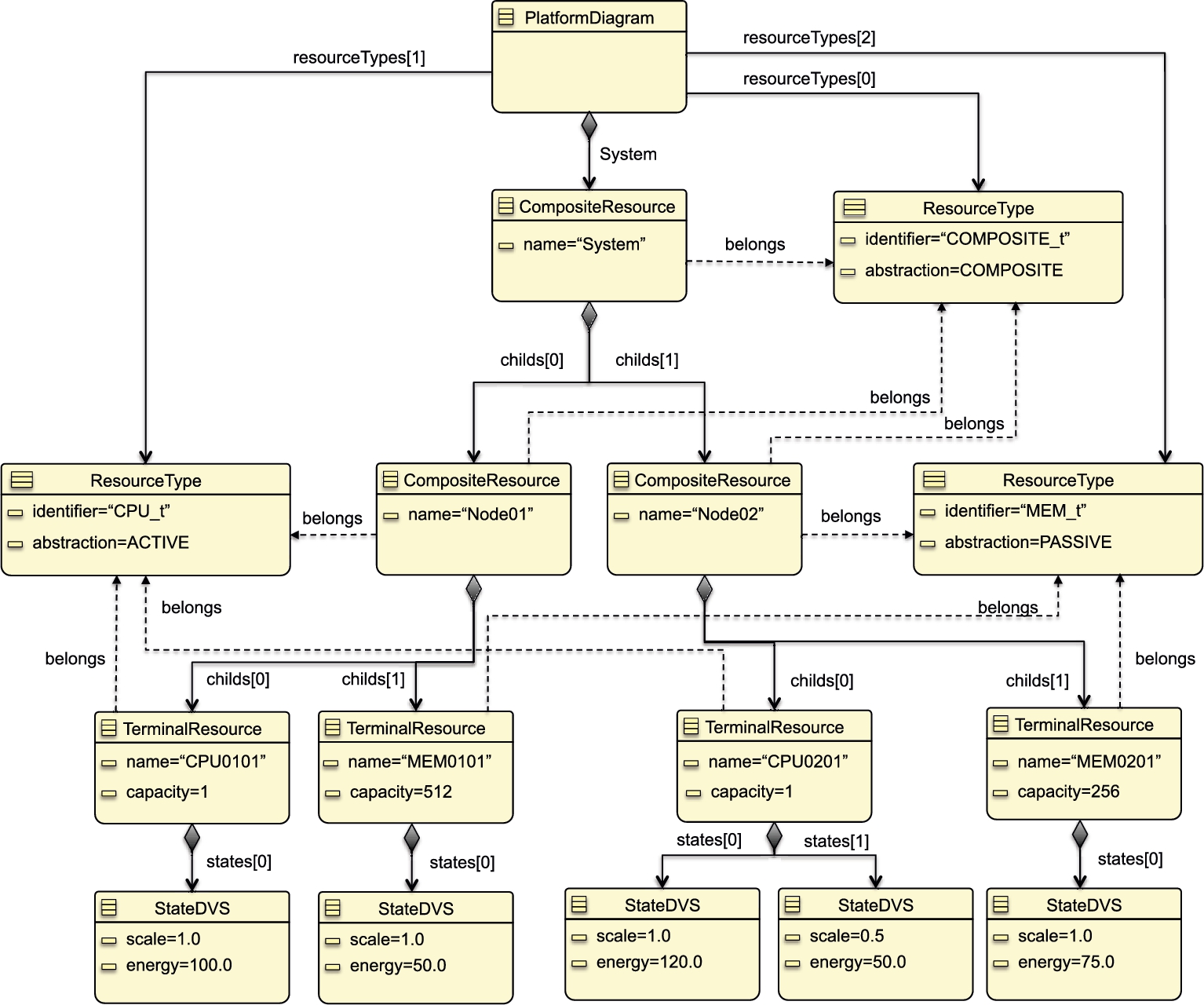
Appendix 9.B Platform model
The metamodel shown in Fig. 9.5 is instantiated according to the registration system given in Section 9.2. To this aim, we define a platform model depicted in Fig. 9.15 in which the system has two composite resources, each of which consists of one active and one passive resource. Each terminal resource has one state except the active resource of the second composite resource. There exist three resource types: processing unit (active), memory (passive), and computation node (composite). Unlike the other terminal resources, the processing unit of the second node has two states: half- and full-speed running modes. Each processing unit has a unit capacity. The memory components have 512- and 256-unit capacity on the first and second computation nodes, respectively.
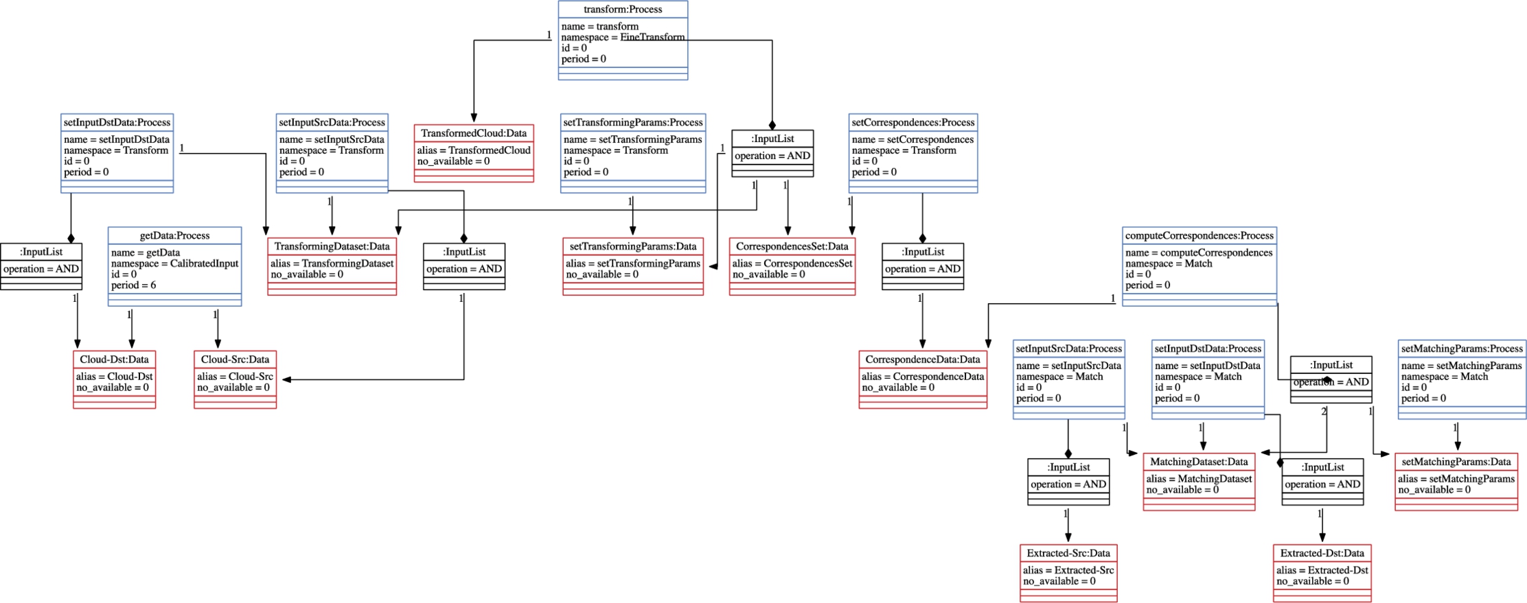
Appendix 9.C Process model
In Figs. 9.16 and 9.17, the process model is presented which is created from the Process metamodel presented in Fig. 9.6 in Section 9.4.4. Since the process model is rather large, in the figure, we will only elaborate a selected set of processes. As explained previously, the input data are acquired by utilizing the class Input. For this purpose, the operation getData is defined. In some cases, the accuracy of acquired data may be crucial. To this aim, the class CalibratedInput is used instead of using the superclass of it. The operation calibrate aims to increase the quality of the data if it is called before calling getData.
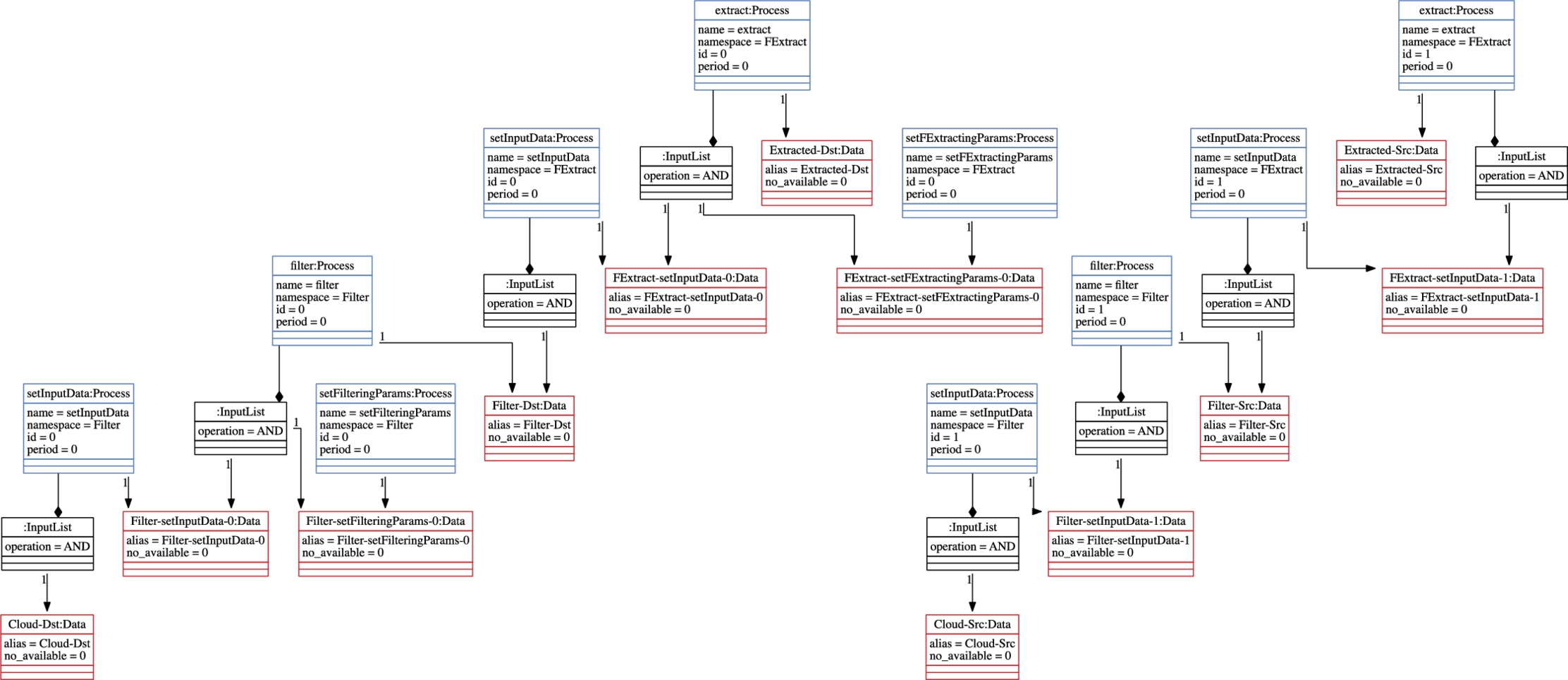
To reduce the size of the input data, the class Filter is defined. The operation setInputData is used to set the interested data. To set the filtering-related parameters, the operation setFilteringParams is defined. The operation filter is, finally, called to gather the filtered data. The class Filter is specialized further into classes NoiseRemoval and Sampling, which are responsible for eliminating the erroneous data and getting a part of the data to reduce the size, respectively. Classes inheriting to these classes, such as StatisticalOutlierRemoval or VoxelGrid, correspond to the different algorithmic approaches.
The class FExtract is responsible for computing predefined key features of the data to reason about the geometric properties. Similarly, the operation setInputData of the class FExtract is utilized to set the interested data, and the operation setFExtractingParams is responsible to adjust the settings of the class. To gather a combination of computed key features and the given data, the operations extract is called. Classes NARF, SIFT, and FPFH represent the definitions for computing various predefined features.
To relate two different inputs to each other, the class Match is defined. One of the important factors that is supposed to be decided is the direction of the relation from source to destination data, which are set with the operations setInputSrcData and setInputDstData, respectively. The relevant parameters are adjusted using the operation setMatchingParams. The operation computeCorrespondences is responsible for obtaining the related data in pairs.
To transform the source data into the coordinate frame of the destination data, class Transform is utilized. Similar to class Match, it has two operations, setInputSrcData and setInputDstData, for setting source and destination data. The operation setTransformingParams is used to configure the parameters. To increase the accuracy of a transformation process, the computed correspondences can be given using setCorrespondences. The operation getTransformationMatrix gives the transformation matrix including rotation and translation. This class is specialized into two classes, CoarseTransform and FineTransform. In the literature [48], the coarse transform is known as the preprocess initial alignment to pretransforming the data to increase the accuracy of the process. In some cases, there may be no need for further transformation after initial alignment, but mostly to gather accurate results, the process fine transformation is applied. The classes CoarseTransform and FineTransform have two different operations, align and transform, respectively, to perform their own computation and set the transformation matrix, accordingly. The class Coarse Transform is specialized further into two different approaches, FPCA_IA and SAC_IA. The class ICP, called iterative closest point, is a commonly known algorithm. Classes LinearICP and NLinearICP correspond to the different versions of ICP algorithms.
Appendix 9.D The instantiation of the value metamodel for energy consumption and computation accuracy
In this section we will illustrate how the Value metamodel that is presented in Fig. 9.7 of Section 9.4.5 is instantiated for the two quality attributes energy reduction and precision.
The instantiation parameters are shown in Table 9.2, where the rows and columns represent the features defined in the feature model and the values for the quality attributes, respectively. In the figure, each cell includes the positive and negative contributions of the feature to the process configuration. Since the operations are not specifically defined in the value models, the contributions of operations are the same with the contributions of the owner class defined in the class model. The higher values for energy model and precision model mean that the corresponding feature increases the energy consumption and decreases the computation accuracy, respectively.
Table 9.2
| Energy value | Precision value | |
|---|---|---|
| Registration | 0 / 0 | 0 / 0 |
| Input | 0 / 0 | 0 / 0 |
| CalibratedInput | 50 / 30 | 20 / 50 |
| Filter | 5 / 0 | 5 / 10 |
| NoiseRemoval | 10 / 0 | 10 / 20 |
| PassthroughFilter | 15 / 0 | 15 / 30 |
| RadiusOutlierRemoval | 15 / 0 | 15 / 30 |
| StatisticalOutlierRemoval | 15 / 0 | 15 / 30 |
| Sampling | 10 / 0 | 10 / 20 |
| VoxelGrid | 15 / 0 | 15 / 30 |
| Uniform | 15 / 0 | 15 / 30 |
| FExtract | 10 / 0 | 5 / 10 |
| SIFT | 30 / 0 | 10 / 30 |
| NARF | 30 / 0 | 10 / 30 |
| FPFH | 30 / 0 | 10 / 30 |
| Match | 20 / 0 | 15 / 50 |
| Transform | 5 / 0 | 5 / 5 |
| CoarseTransform | 10 / 0 | 10 / 30 |
| FPCA_IA | 12 / 0 | 5 / 30 |
| SAC_IA | 12 / 0 | 5 / 30 |
| FineTransform | 15 / 0 | 2 / 90 |
| ICP | 15 / 0 | 3 / 90 |
| LinearICP | 20 / 0 | 1 / 110 |
| NLinearICP | 20 / 0 | 1 / 110 |