
CHAPTER 23
Using Data Validation
This chapter explores a useful Excel feature: data validation. Data validation enables you to add rules for what's acceptable in specific cells, and it allows you to add dynamic elements to your worksheet without using any macro programming.
About Data Validation
The Excel data validation feature allows you to set up rules that determine what can be entered into a cell. For example, you may want to limit data entry in a particular cell to whole numbers between 1 and 12. If the user makes an invalid entry, you can display a custom message, such as the one shown in Figure 23.1.

FIGURE 23.1 Displaying a message when the user makes an invalid entry
Excel makes it easy to specify the validation criteria. You can also use a formula for more complex criteria.
Specifying Validation Criteria
To specify the type of data allowable in a cell or range, follow these steps:
- Select the cell or range of cells.
- Choose Data ➪ Data Tools ➪ Data Validation. The Data Validation dialog box appears, as shown in Figure 23.2.

FIGURE 23.2 The three tabs of the Data Validation dialog box
- Select the Settings tab.
- Choose an option from the Allow drop-down list. The contents of the Data Validation dialog box change, displaying controls based on your choice. For example, to specify a formula, select Custom.
- Specify the conditions by using the displayed controls. Your selection in step 4 determines the other controls that you can access.
- (Optional) Select the Input Message tab and specify which message to display when a user selects the cell. You can use this optional step to tell the user what type of data is expected or to document the purpose of the cell. If this step is omitted, no message will appear when the user selects the cell.
- (Optional) Select the Error Alert tab and specify which error message to display when a user makes an invalid entry. The selection for Style determines what choices users have when they make invalid entries. For example, choose Stop to prevent an invalid entry. If this step is omitted, a standard message will appear if the user makes an invalid entry.
- Click OK. The cell or range contains the validation criteria you specified.
Types of Validation Criteria You Can Apply
From the Settings tab of the Data Validation dialog box, you can specify a variety of data validation criteria. The following options are available from the Allow drop-down list. Keep in mind that the other controls on the Settings tab vary, depending on your choice from the Allow drop-down list.
- Any Value Selecting this option removes any existing data validation. Note, however, that the input message, if any, still is displayed if the box is checked on the Input Message tab.
- Whole Number The user must enter a whole number. You specify a valid range of whole numbers by using the Data drop-down list. For example, you can specify that the entry must be a whole number greater than or equal to 100.
- Decimal The user must enter a number. You specify a valid range of numbers by refining the criteria from choices in the Data drop-down list. For example, you can specify that the entry must be between 0 and 1.
- List The user must choose from a list of entries that you provide. Type a comma-separated list of values in the Source text box. This option is useful, and we discuss it in detail later in this chapter. (See “Creating a Drop-Down List.”)
- Date The user must enter a date. You specify a valid date range from the choices in the Data drop-down list. For example, you can specify that the data entered must be greater than or equal to January 1, 2022.
- Time The user must enter a time. You specify a valid time range from choices in the Data drop-down list. For example, you can specify that the data entered must be greater than 12:00 PM.
- Text Length The length of the data (number of characters) is limited. You specify a valid length by using the Data drop-down list and the Length text box. For example, you can specify that the length of the data entered be 1 (a single alphanumeric character).
- Custom To use this option, you must supply a logical formula that determines the validity of the user's entry. (A logical formula returns either
TRUEorFALSE.) You can enter the formula directly into the Formula control (which appears when you select the Custom option), or you can specify a cell reference that contains a formula. This chapter contains examples of useful formulas.
The Settings tab of the Data Validation dialog box contains these other check boxes:
- Ignore Blank If this is selected, blank entries are not circled as invalid when using Data ➪ Data Tools ➪ Data Validation ➪ Circle Invalid Data.
- In-Cell Dropdown If you select List in the Allow drop-down list, you can choose to show or hide a drop-down arrow in the cell to aid the user in the selecting a valid value.
- Apply These Changes to All Other Cells with the Same Settings If this is selected, the changes that you make apply to all other cells that contain the original data validation criteria.
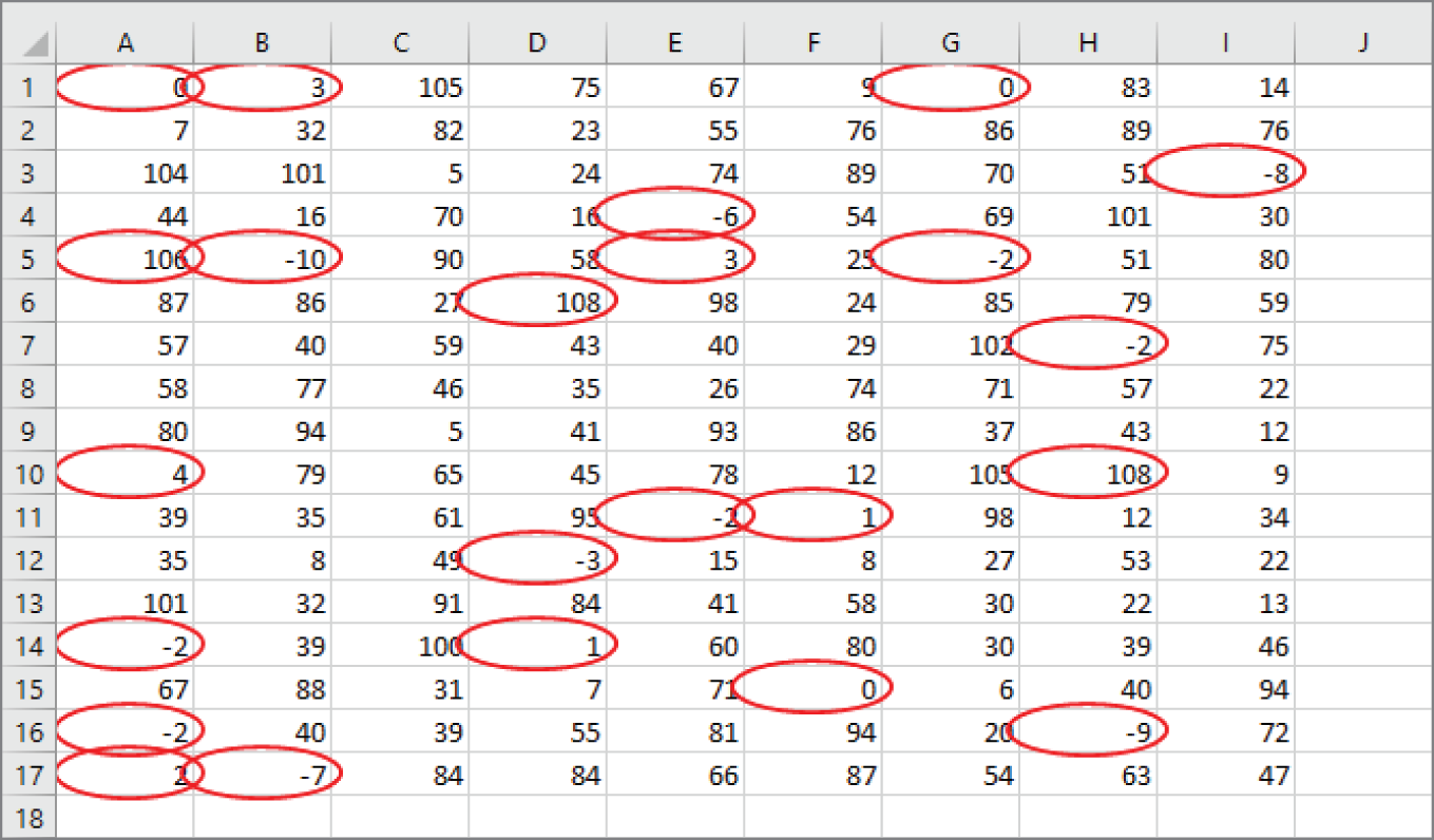
FIGURE 23.3 Excel can draw circles around invalid entries (in this case, cells that aren't between 5 and 105).
Creating a Drop-Down List
One of the most common uses of data validation is to create a drop-down list in a cell. Figure 23.4 shows an example that uses region names in cells A2:A6 as the list source.
To create a drop-down list in a cell, follow these steps:
- Enter the list items into a single-row or single-column range. These items will appear in the drop-down list.
- Select the cell that will contain the drop-down list and then choose Data ➪ Data Tools ➪ Data Validation. The Data Validation dialog box appears.
- From the Settings tab, select the List option (from the Allow drop-down list) and specify the range that contains the list, using the Source control. The range can be in a different worksheet, but it must be in the same workbook.
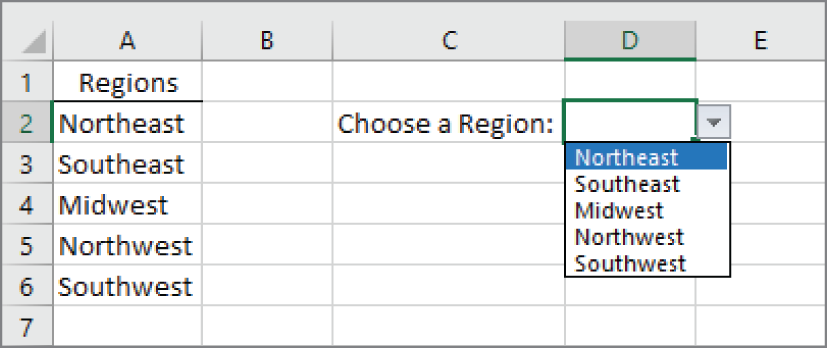
FIGURE 23.4 This drop-down list was created using data validation.
- Make sure that the In-Cell Dropdown check box is selected.
- Set any other Data Validation options as desired.
- Click OK. The cell displays an input message (if specified) and a drop-down arrow when it's selected.
- Click the arrow and choose an item from the list that appears.
Unfortunately, you cannot control the font size used in drop-down lists. If the cell that displays the drop-down is formatted to show large text, the drop-down list does not use that formatting. If you zoom out on a worksheet, it may be difficult to read the items.
Using Formulas for Data Validation Rules
For simple data validation, the data validation feature is quite straightforward and easy to use. The real power of this feature, though, becomes apparent when you use the Custom option and supply a formula.
The formula that you specify must be a logical formula that returns either TRUE or FALSE. If the formula evaluates to TRUE, the data is considered valid and remains in the cell. If the formula evaluates to FALSE, a message box appears that displays the message that you specify on the Error Alert tab of the Data Validation dialog box.
Specify a formula in the Data Validation dialog box by selecting the Custom option from the Allow drop-down list of the Settings tab. Enter the formula directly into the Formula control or enter a reference to a cell that contains a formula. The Formula control appears on the Settings tab of the Data Validation dialog box when the Custom option is selected.
We present several examples of formulas used for data validation in the section “Data Validation Formula Examples” later in this chapter.
Understanding Cell References
If the formula that you enter in the Data Validation dialog box contains a cell reference, that reference is considered a relative reference, based on the upper-left cell in the selected range.
The following example clarifies this concept. Suppose you want to allow only an odd number to be entered into the range B2:B10. None of the Excel data validation rules can limit entry to odd numbers, so a formula is required.
Follow these steps:
- Select the range (
B2:B10in this example) and make sure that cell B2 is the active cell. - Choose Data ➪ Data Tools ➪ Data Validation. The Data Validation dialog box appears.
- Select the Settings tab and select the Custom option (from the Allow drop-down list).
- Enter the following formula in the Formula field, as shown in Figure 23.5:
=ISODD(B2)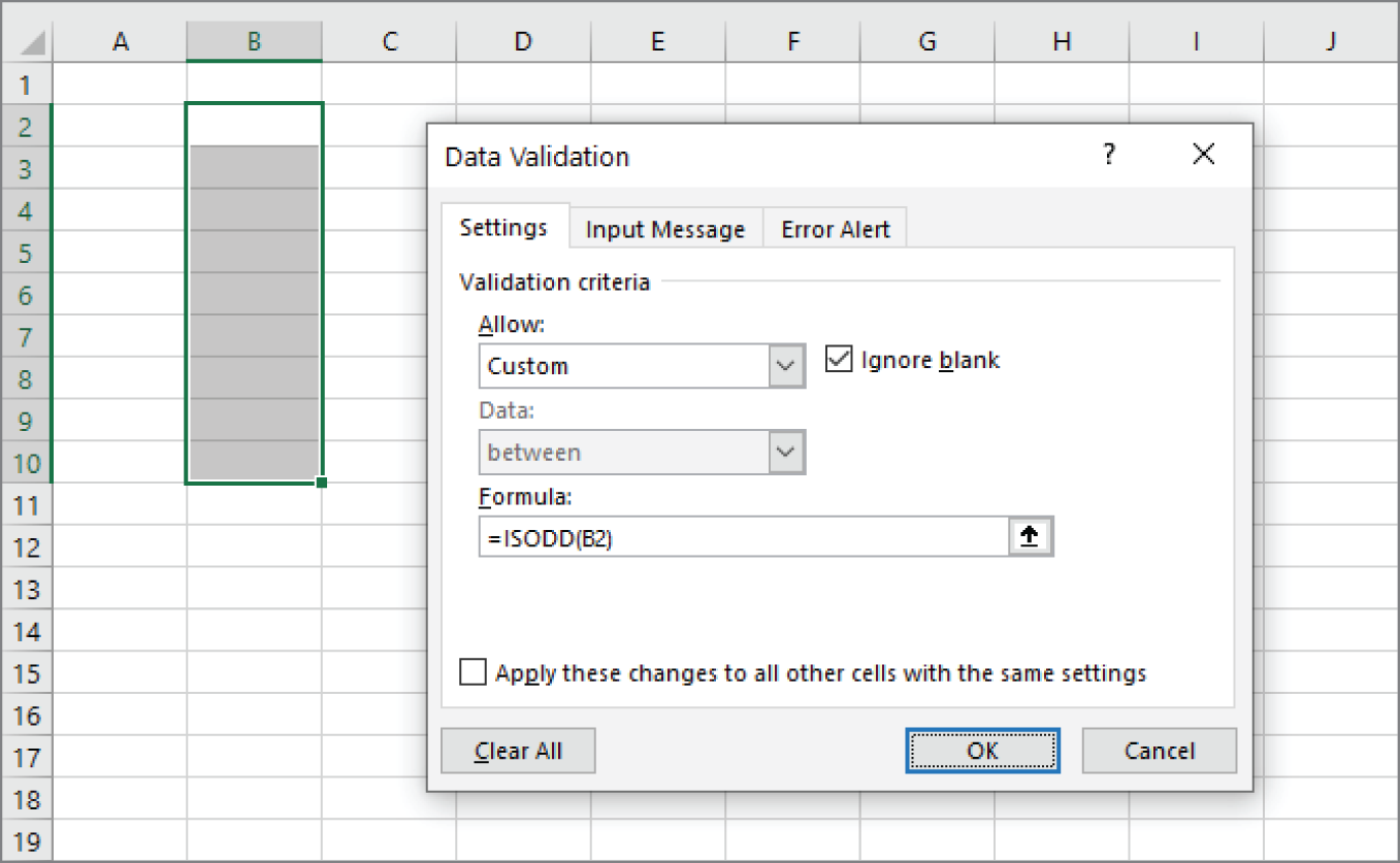
FIGURE 23.5 Entering a data validation formula
This formula uses the
ISODDfunction, which returnsTRUEif its numeric argument is an odd number. Notice that the formula refers to the active cell, which is cell B2. - On the Error Alert tab, choose Stop for the Style and then type
An odd number is required herein the Error Message field. - Click OK to close the Data Validation dialog box.
Notice that the formula entered contains a reference to the upper-left cell in the selected range. This data validation formula was applied to a range of cells, so you might expect that each cell would contain the same data validation formula. Because you entered a relative cell reference as the argument for the ISODD function, Excel adjusts the formula for the other cells in the B2:B10 range. To demonstrate that the reference is relative, select cell B5 and examine its formula displayed in the Data Validation dialog box. You'll see that the formula for this cell is:
=ISODD(B5)Generally, when entering a data validation formula for a range of cells, you use a reference to the active cell, which is normally the upper-left cell in the selected range. An exception is when you need to refer to a specific cell. For example, suppose that you select range A1:B10 and you want your data validation to allow only values that are greater than the value in cell C1. You would use this formula:
=A1>$C$1In this case, the reference to cell C1 is an absolute reference; it will not be adjusted for the cells in the selected range, which is just what you want. The data validation formula for cell A2 looks like this:
=A2>$C$1The relative cell reference is adjusted, but the absolute cell reference is not.
Data Validation Formula Examples
The following sections contain a few data validation examples that use a formula entered directly into the Formula control on the Settings tab of the Data Validation dialog box. These examples help you understand how to create your own data validation formulas.
Accepting text only
Excel has a data validation option to limit the length of text entered into a cell, but it doesn't have an option to force text (rather than a number) into a cell. To force a cell or range to accept only text (no values), use the following data validation formula:
=ISTEXT(A1)This formula assumes that the active cell in the selected range is cell A1.
Accepting a larger value than the previous cell
The following data validation formula enables the user to enter a value only if it's greater than the value in the cell directly above it:
=A2>A1This formula assumes that A2 is the active cell in the selected range. Note that you can't use this formula for a cell in row 1.
Accepting nonduplicate entries only
The following data validation formula does not permit the user to make a duplicate entry in the range A1:C20
:
=COUNTIF($A$1:$C$20,A1)=1This is a logical formula that returns TRUE if the value in the cell occurs only one time in the A1:C20 range. Otherwise, it returns FALSE, and the Duplicate Entry dialog box is displayed.
This formula assumes that A1 is the active cell in the selected range. Note that the first argument for COUNTIF is an absolute reference. The second argument is a relative reference, and it adjusts for each cell in the validation range. Figure 23.6 shows this validation criterion in effect using a custom error alert message. The user is attempting to enter 12 into cell B5.
Accepting text that begins with a specific character
The following data validation formula demonstrates how to check for a specific character. In this case, the formula ensures that the user's entry is a text string that begins with the letter A (uppercase or lowercase):
=LEFT(A1)="a"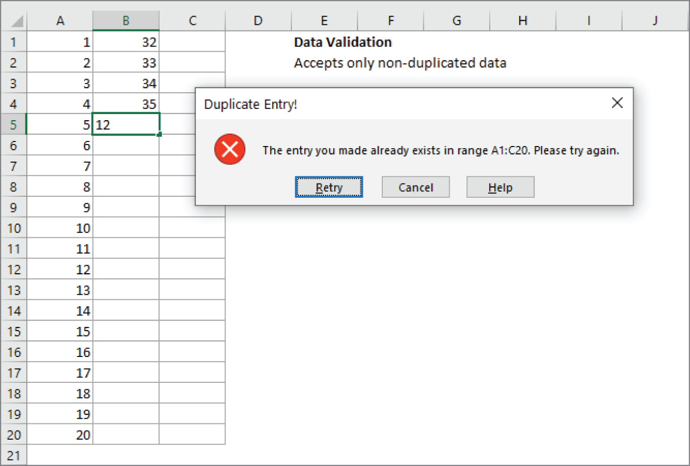
FIGURE 23.6 Using data validation to prevent duplicate entries in a range
This is a logical formula that returns TRUE if the first character in the cell is the letter A. Otherwise, it returns FALSE. This formula assumes that the active cell in the selected range is cell A1.
The following formula is a variation of this validation formula. It uses wildcard characters in the second argument of the COUNTIF function. In this case, the formula ensures that the entry begins with the letter A and contains exactly five characters:
=COUNTIF(A1,"A????")=1Accepting dates by the day of the week
The following data validation formula assumes that the cell entry is a date, and it ensures that the date is a Monday:
=WEEKDAY(A1)=2This formula assumes that the active cell in the selected range is cell A1. It uses the WEEKDAY function, which returns 1 for Sunday, 2 for Monday, and so on. Note that the WEEKDAY function accepts any non-negative value as an argument (not just dates).
Accepting only values that don't exceed a total
Figure 23.7 shows a simple budget worksheet, with the budget item amounts in the range B1:B6. The planned budget is in cell E5, and the user is attempting to enter a value in cell B4 that would cause the total (cell E6) to exceed the budget. The following data validation formula ensures that the sum of the budget items does not exceed the budget:
=SUM($B$1:$B$6)<=$E$5 
FIGURE 23.7 Using data validation to ensure that the sum of a range does not exceed a certain value
Creating a dependent list
As we described previously, you can use data validation to create a drop-down list in a cell (see “Creating a Drop-Down List” earlier in this chapter). This section explains how to use a drop-down list to control the entries that appear in a second drop-down list. In other words, the second drop-down list is dependent upon the value selected in the first drop-down list.
Figure 23.8 shows a simple example of a dependent list created by using data validation. Cell E2 contains data validation that displays a three-item list from the range A1:C1 (Vegetables, Fruits, and Meats). When the user chooses an item from the list, the second list (in cell F2) displays the appropriate items.
This worksheet uses three named ranges:
- Vegetables:
A2:A15 - Fruits:
B2:B9 - Meats:
C2:C5
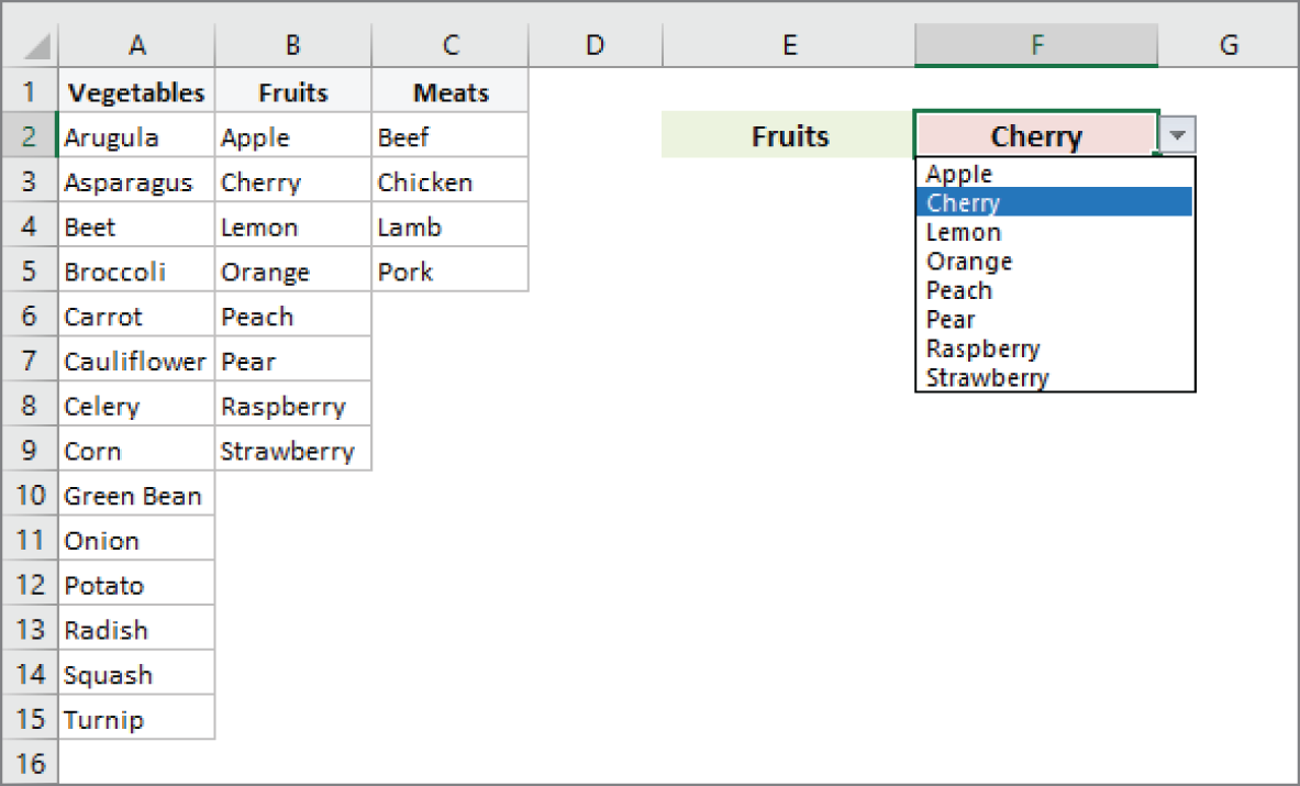
FIGURE 23.8 The items displayed in the list in cell F2 depend on the list item selected in cell E2.
Cell F2 contains data validation that uses this formula:
=INDIRECT($E$2)Therefore, the drop-down list displayed in F2 depends on the value displayed in cell E2.
Using Data Validation without Restricting Entry
The most common use of data validation is to prevent a user from entering invalid data. But data validation can also be used as a component of your spreadsheet's user interface without restricting the user's entry. The two examples of showing an input message and making suggestions would require quite a bit of VBA programming to accomplish, but it can be accomplished easily with data validation.
Showing an input message
Data validation provides a way to display a message when the user selects a cell. Normally, this message would tell the user what would be considered invalid data for that cell to prevent them from getting the error message if they enter invalid data. But you can use this message for anything.
Figure 23.9 shows an input message reminding the user to complete a previous step. The Allow drop-down list is set to Any Value, so the user is not prevented from entering anything into this cell. It's just a reminder set to a cell that the user will likely use early in the process of completing this workbook.
Making suggested entries
The default Style value on the Error Alert tab of the Data Validation dialog box is Stop. This not only displays a message, but it also prevents the user from completing the entry of invalid data. There are two other options, Warning and Information, which will allow the user to enter any data. You can also deselect the check box and Excel will not show any message.
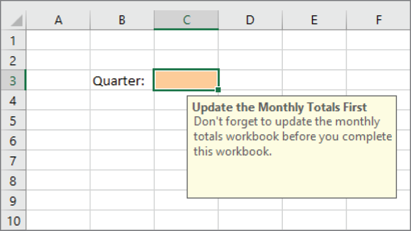
FIGURE 23.9 Data validation can be used to show messages to the user.
Suppose that you have a field where the user is to enter the name of a fruit. To help the user, you provide a list of common fruits, but you want the user to be able to enter fruits that aren't on the list. The list is merely there to save the user some typing if they need to enter a common fruit.
To set up this scenario, select List and point to the list of fruits, as shown in Figure 23.10. Then uncheck the Show Error Alert After Invalid Data Is Entered check box on the Error Alert tab. Now the user can select from the list or type in a fruit that's not on the list. Of course, you can't prevent the user from typing in nonsense.
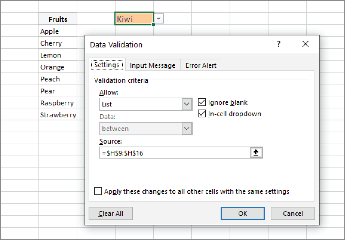
FIGURE 23.10 Data Validation dialog box