
CHAPTER 22
Importing and Cleaning Data
Data is everywhere. For example, if you run a website, you're collecting data continually, and you may not even know it. Every visit to your site generates information that is stored in a file on your server. This file contains lots of useful information if you take the time to examine it.
That's just one example of data collection. Virtually every automated system collects data and stores it. Most of the time, the system that collects the data is also equipped to verify and analyze the data—but not always. And, of course, data is also collected manually. A nonautomated telephone survey is a good example.
Excel is a good tool for analyzing data, and it's often used to summarize the information and display it in the form of tables and charts. But often, the data that's collected isn't perfect. For one reason or another, it needs to be cleaned up before it can be analyzed.
Excel is a great tool for cleaning up data. Cleaning data involves getting raw data into a worksheet and then manipulating it so that it conforms to your requirements. In the process, the data will be made consistent so that it can be properly analyzed.
This chapter describes the various ways to get data into a worksheet, and it provides some tips to help you clean it up.
Importing Data
The first step is to get the data into a worksheet. Excel can import most common text file formats, including data from websites.
Importing from a file
The following sections describe the file types that Excel can open directly, using the File ➪ Open command. Figure 22.1 shows the list of file filter options that you can specify in the Open dialog box.
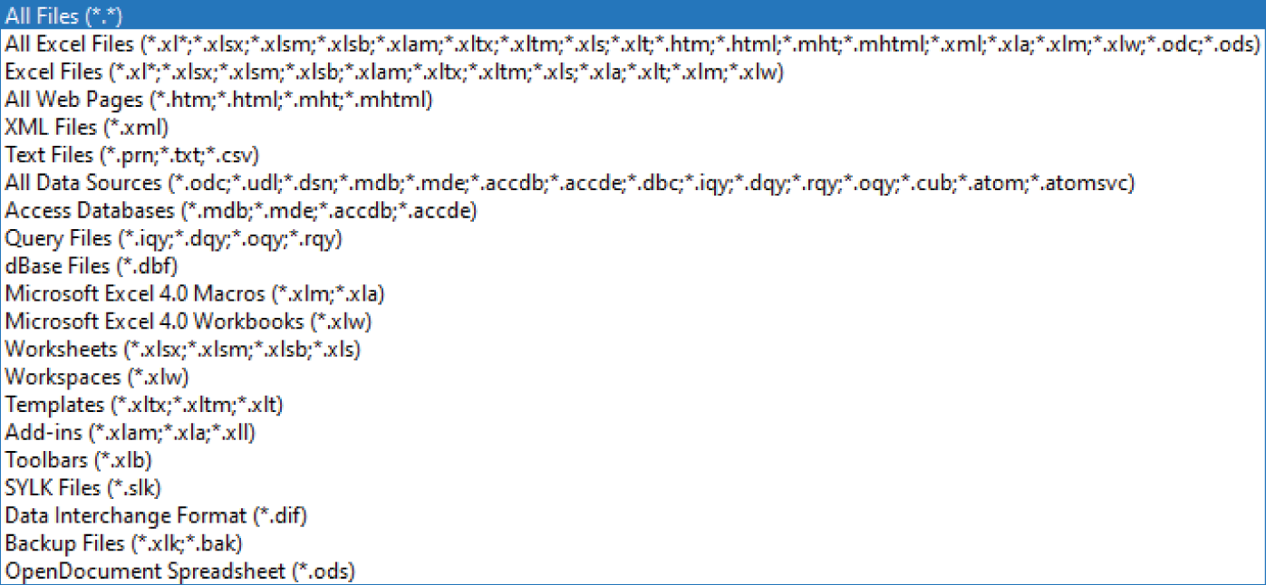
FIGURE 22.1 Filtering by file extension in the Open dialog box
Spreadsheet file formats
In addition to the current file formats (XLSX, XLSM, XLSB, XLTX, XLTM, and XLAM), Excel can open workbook files from all previous versions of Excel:
- XLS: Binary files created by Excel 4, Excel 95, Excel 97, Excel 2000, Excel 2002, and Excel 2003
- XLM: Binary files that contain Excel 4 macros (no data)
- XLT: Binary files for an Excel template
- XLA: Binary files for an Excel add-in
Excel can also open ODS files (the OpenDocument Spreadsheet format) created by other spreadsheet products. ODS files are produced by a variety of “open” software programs, including Google Sheets, Apache OpenOffice, LibreOffice, and several others.
Database file formats
Excel can open the following database file formats:
- Access files: The names of these files have various extensions, including
.mdband.accdb. - dBase files: These files are produced by dBase III and dBase IV and have names with a
.dbfextension. Excel does not support dBase II files.
When you try to open database files using File ➪ Open, Excel doesn't actually open the file. Instead, it creates an external data connection to the table in the database that you select. Excel supports various types of database connections that enable you to access data selectively. For example, instead of “opening” a database and selecting a table, you can perform a query on a table to retrieve only the records that you need (rather than the entire table).
Text file formats
A text file contains raw characters with no formatting. Excel can open most types of text files:
- CSV: This stands for “comma-separated values.” Columns are delimited with a comma, and rows are delimited with a carriage return.
- TXT: Columns are delimited with a tab, and rows are delimited with a carriage return.
- PRN: Columns are delimited with multiple space characters, and rows are delimited with a carriage return. Excel imports this type of file into a single column.
- DIF: This file format (DIF stands for Data Interchange Format) was originally used by the VisiCalc spreadsheet. This is rarely used.
- SYLK: This file format (SYLK stands for Symbolic Link and the filenames have the
.slkextension) was originally used by Multiplan. This is rarely used.
Most of these text file types have variants. For example, text files produced on a Mac have different end-of-row characters. Excel can usually handle the variants without a problem.
When you attempt to open a text file in Excel, the Text Import Wizard might kick in to help you specify how you want the data to be retrieved.
HTML files
Excel can open most HTML files, which can be stored on your local drive or on a web server. The way that the HTML code renders in Excel varies considerably. Sometimes, the HTML file may look exactly as it does in a browser. At other times, it may bear little resemblance, especially if the HTML file uses Cascading Style Sheets (CSS) for its layout.
In some cases, you can access data on the Web by using Power Query. We discuss this topic in Part V, “Understanding Power Pivot and Power Query.”
XML files
Extensible Markup Language (XML) is a text file format suitable for structured data. Data is enclosed in tags, which also serve to describe the data.
Excel can open XML files and simpler ones will be displayed with little or no effort. Complex XML files will require some work, however. A discussion of this topic is beyond the scope of this book. You'll find information about getting data from XML files in Excel's Help system and online.
Importing vs. opening
When you use File ➪ Open to open a file that's not in a traditional Excel format, you may be opening the file, or you may be importing it, depending on the file type. As mentioned, database files aren't opened. Rather, a table from inside the database file is imported.
XML files are another example of a format that may not open directly. When you open an XML file, you have the choice of opening it as a read-only workbook or importing it into a table.
Text files are opened directly. Excel understands CSV files, so it doesn't have to ask you any questions when you open them. For tab-delimited or fixed-width files, the Text Import Wizard will guide you in identifying where the data begins and ends.
When a file is opened directly, the Excel title bar will show the file's name. Figure 22.2 shows the Excel title bar after a file named reunion.txt was opened. When the File ➪ Open process actually imports the data, it's imported into a new workbook. In that case, the title bar will have a generic new workbook name, like Book1.
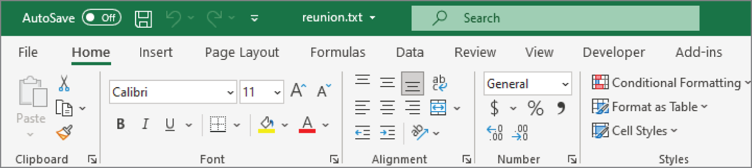
FIGURE 22.2 Excel's title bar displays the opened file's name.
Importing a text file
One of the advantages of importing a text file instead of opening it is that you can put the data into a specific range in a worksheet rather than starting in cell A1. In this example, we'll show you how to import a text file to a specific range, and we'll walk through the steps of the Text Import Wizard.
Text files can be delimited or fixed-width. In delimited files, a character (like a comma or a tab) separates the columns. In fixed-width, each column occupies the same number of characters, and spaces are used to pad the data. For example, a fixed-width file whose first column is 20 characters long means that the second column always starts at the 21st character. The example in this section imports a file delimited by commas, but the process for importing fixed width is similar.
Beginning with Excel 2019, importing text files is done through Get & Transform rather than the legacy Text Import Wizard. Get & Transform is a powerful feature, and we discuss it at length in Part V, “Understanding Power Pivot and Power Query.” For this example, however, we're going to use the legacy wizard. With all of Get & Transform's power, it took away some flexibility like not having a header row. It's valuable to know both ways of importing text files.
Before we begin, we have to enable the legacy wizard. To do that, choose File ➪ Options ➪ Data and check From Text (Legacy), as shown in Figure 22.3. This will add the necessary menu item for the next step.
Figure 22.4 shows a small CSV file. The following instructions describe how to import this file, named monthly.csv, beginning at cell C3.
- Choose Data ➪ Get & Transform Data ➪ Get Data ➪ Legacy Wizards ➪ From Text (Legacy). The Import Text File dialog box appears.
- Navigate to the folder that contains the text file.
- Select the file from the list and then click the Import button. The Text Import Wizard appears, as shown in Figure 22.5.
- Select Delimited and make sure that the My Data Has Headers check box is unchecked. Click Next to go to step 2.
- Choose Comma as the delimiter and uncheck any others (see Figure 22.6).
- Click the Finish button. The Import Data dialog box appears, as shown in Figure 22.7.
- In the Import Data dialog box, specify the location for the imported data. It can be a cell in an existing worksheet or a new worksheet.
- Click OK, and Excel imports the data (see Figure 22.8).

FIGURE 22.3 Enabling the legacy import wizard
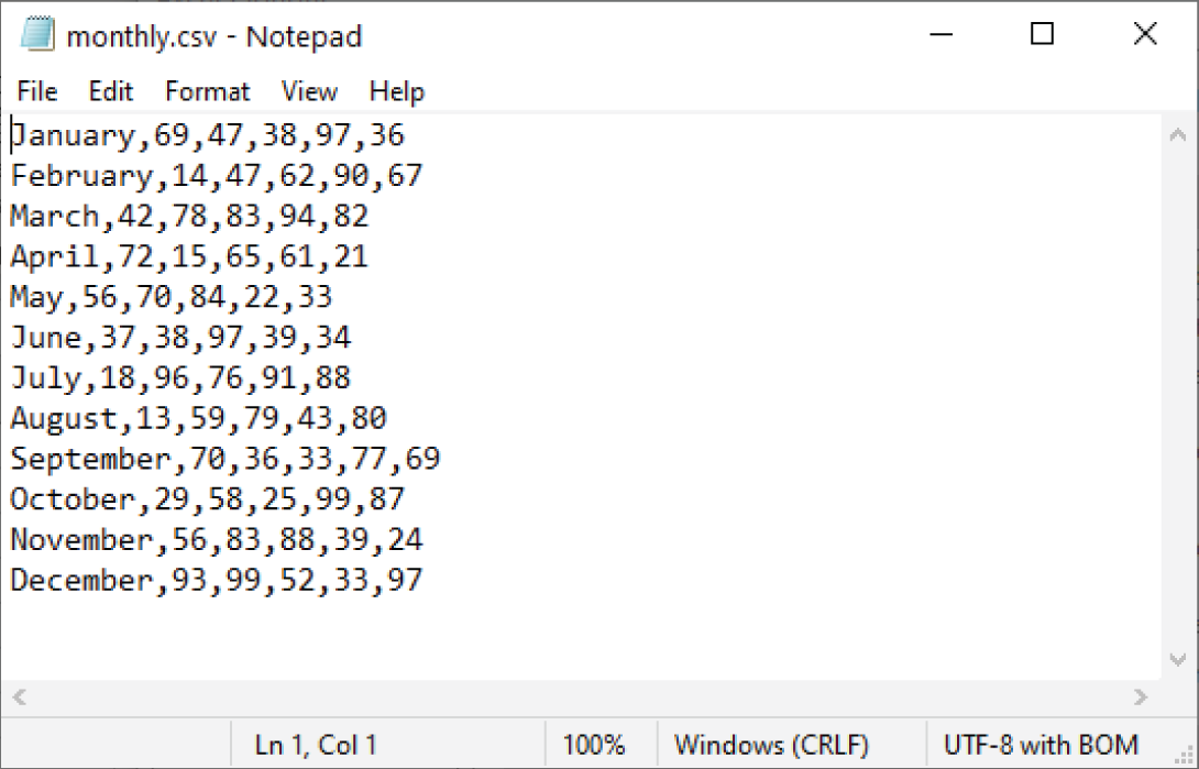
FIGURE 22.4 This CSV file will be imported.
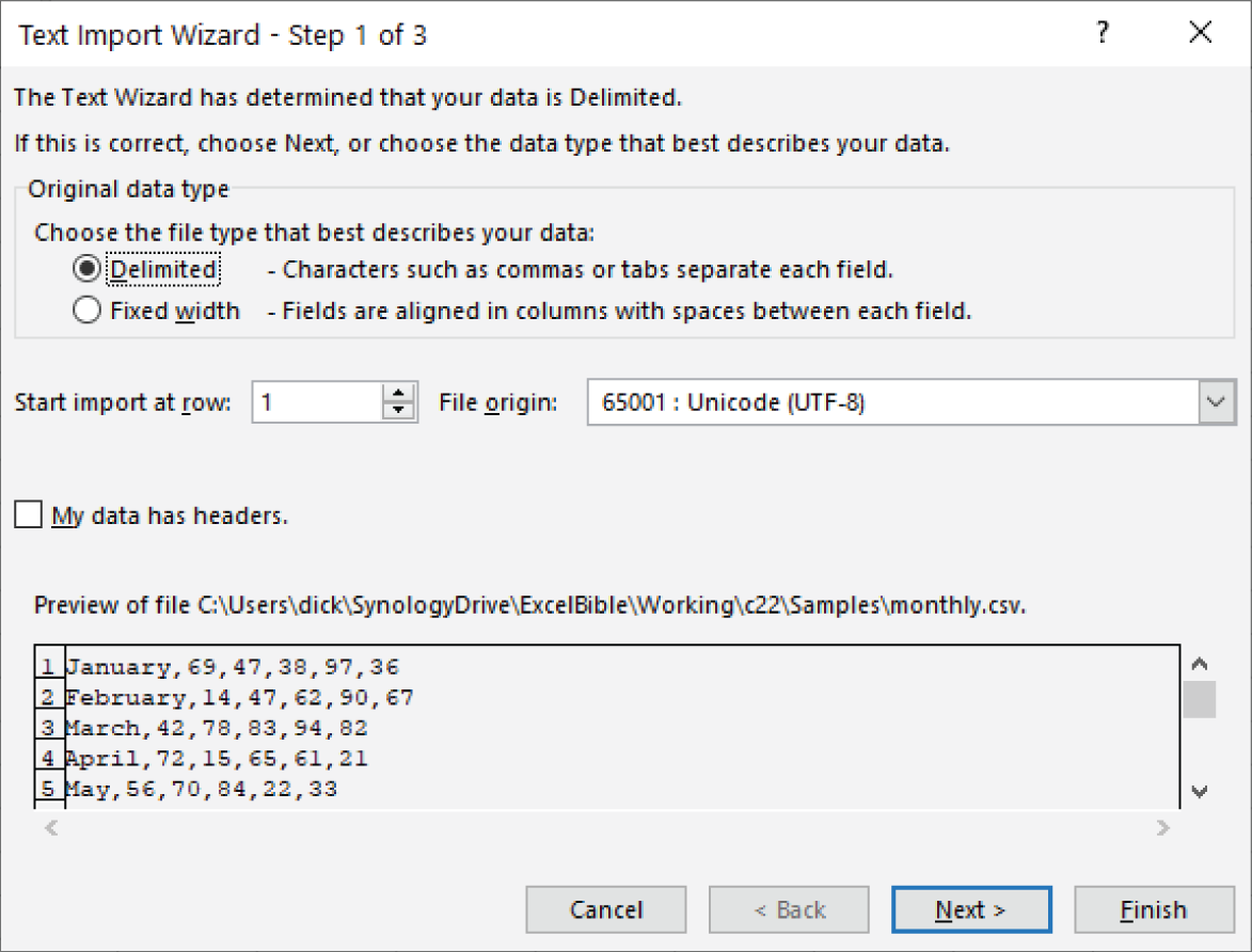
FIGURE 22.5 Step 1 of the Text Import Wizard
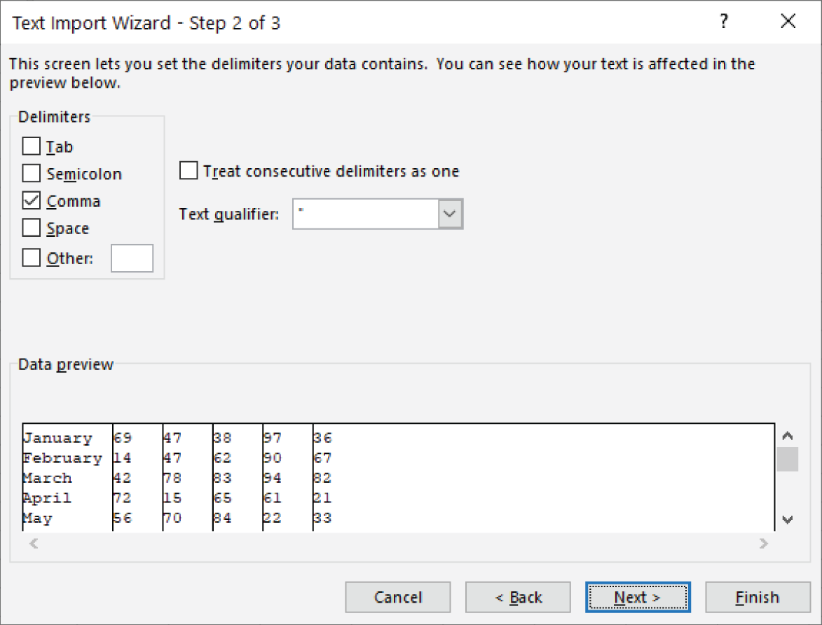
FIGURE 22.6 Select the delimiter in step 2 of the Text Import Wizard.

FIGURE 22.7 Using the Import Data dialog box to import a CSV file
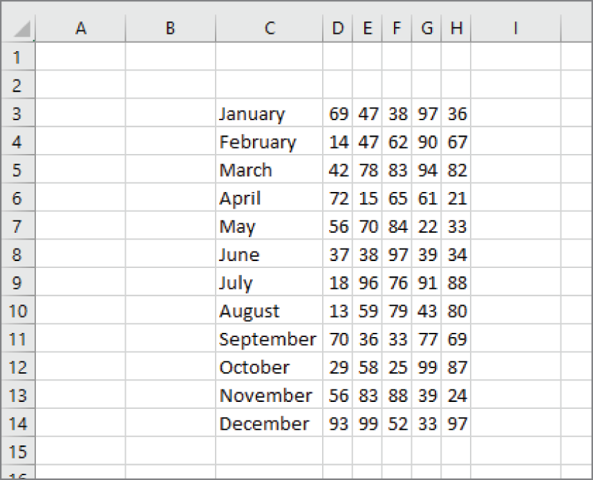
FIGURE 22.8 This range contains data imported directly from a CSV file.
Copying and pasting data
If all else fails, you can try standard copy-and-paste techniques. If you can copy data from an application (for example, a word-processing program or a document displayed in a PDF viewer), there's a good chance that you can paste it into an Excel workbook. For the best results, try pasting using the Home ➪ Clipboard ➪ Paste ➪ Paste Special command, and try the various paste options listed. Usually, pasted data will require some cleanup.
Cleaning Up Data
The following sections discuss a variety of techniques that you can use to clean up data in a worksheet.
Removing duplicate rows
If data is compiled from multiple sources, it may contain duplicate rows. Most of the time, you will want to eliminate the duplicates. In the past, removing duplicate data was essentially a manual task—although it could be automated by using a confusing advanced filter technique. But now removing duplicate rows is easy, thanks to Excel's Remove Duplicates command (introduced in Excel 2007).
Start by selecting any cell within your data range. Choose Data ➪ Data Tools ➪ Remove Duplicates, and the Remove Duplicates dialog box, shown in Figure 22.9, appears.
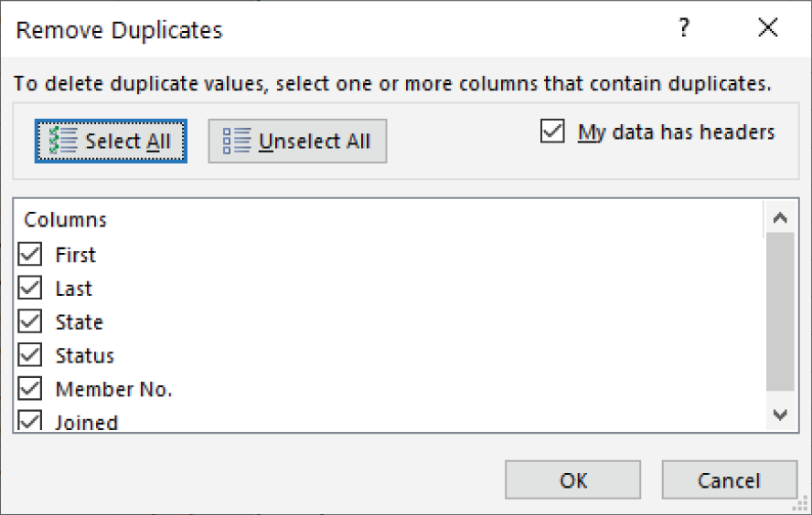
FIGURE 22.9 Use the Remove Duplicates dialog box to delete duplicate rows.
The Remove Duplicates dialog box lists all the columns in your data range or table. Place a check mark next to the columns that you want to be included in the duplicate search. Most of the time, you'll want to select all the columns, which is the default. Click OK, and Excel weeds out the duplicate rows and displays a message that tells you how many duplicates it removed. If Excel deleted too many rows, you can undo the procedure by clicking Undo (or by pressing Ctrl+Z).
When you select all columns in the Remove Duplicates dialog box, Excel will delete a row only if the content of every column is duplicated. In some situations, you may not care about matching some columns, so you would deselect those columns in the Remove Duplicates dialog box. For example, if each row has a unique ID code, Excel would never find any duplicate rows. So, you'd want to uncheck that column in the Remove Duplicates dialog box.
When duplicate rows are found, the first row is kept, and subsequent duplicate rows are deleted.
Identifying duplicate rows
If you would like to identify duplicate rows so that you can examine them without automatically deleting them, here's another method. Unlike the technique described in the previous section, this method looks at actual values, not formatted values.
Create a formula to the right of your data that concatenates each of the cells to the left. The formulas that follow assume that the data is in columns A:F. The TEXTJOIN function in this example separates the columns with a pipe character (usually located above the Enter key on your keyboard).
Enter this formula into cell G2:
=TEXTJOIN("|",FALSE,A2:F2)Add another formula in cell H2. This formula displays the number of times a duplicate value in column G occurs:
=COUNTIF(G:G,G2)Copy these formulas down the column for each row of your data.
Column H displays the number of occurrences of that row. Unduplicated rows will display 1. Duplicated rows will display a number that corresponds to the number of times that row appears.
Figure 22.10 shows a simple example. If you don't care about a particular column, just omit it from the formula in column G. For example, if you want to find duplicates regardless of the Status column, change the formula in G2 to the following:
=TEXTJOIN("|",FALSE,A2:C2,E2:F2) 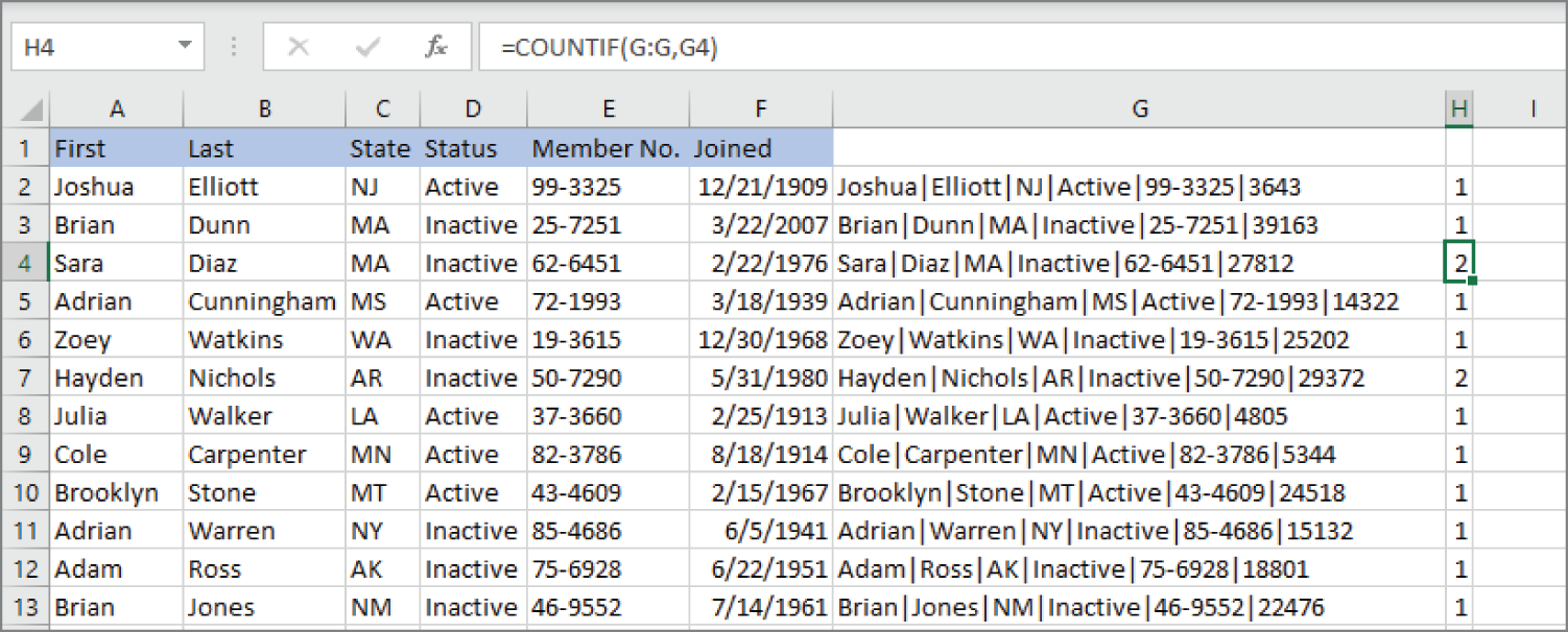
FIGURE 22.10 Using formulas to identify duplicate rows
Splitting text
When importing data, you might find that multiple values are imported into a single column. Figure 22.11 shows an example of this type of import problem.
If the text is all the same length (as in the example), you might be able to write a series of formulas that extract the information to separate columns. The LEFT, RIGHT, and MID functions are useful for this task.
You should also be aware that Excel offers two nonformula methods to assist in splitting data so that it occupies multiple columns: Text to Columns and Flash Fill.
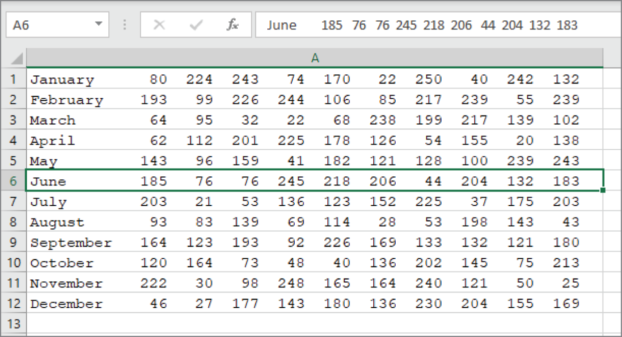
FIGURE 22.11 The imported data was put in one column rather than multiple columns.
Using Text to Columns
The Text to Columns command can parse strings into their component parts.
First, make sure the column that contains the data to be split up has enough empty columns to the right to accommodate the extracted data. Then select the data to be parsed and choose Data ➪ Data Tools ➪ Text to Columns. Excel displays the Convert Text to Columns Wizard, which consists of a series of dialog boxes that walk you through the steps to convert a single column of data into multiple columns. Figure 22.12 shows the initial step, in which you choose the type of data:
- Delimited The data to be split is separated by delimiters such as commas, spaces, slashes, or other characters.
- Fixed Width Each component occupies the same number of characters.
Make your choice and click Next to move on to step 2, which depends on the choice you made in step 1.
If you're working with delimited data, specify the delimiting character. You'll see a preview of the result. If you're working with fixed-width data, specify the column breaks directly in the preview window.
When you're satisfied with the column breaks, click Next to move to step 3. In this step, you can click a column in the preview window and specify formatting for the column. For example, if you have data that looks like a number but is really text, you can format the column as Text so that you preserve any leading zeros. Click Finish, and Excel splits the data as specified.

FIGURE 22.12 The first dialog box in the Convert Text to Columns Wizard
Using Flash Fill
The Text to Columns Wizard works well for many types of data. But sometimes you'll encounter data that can't be parsed by that wizard. For example, the Text to Columns Wizard is useless if you have variable-width data that doesn't have delimiters. In such a case, the Flash Fill feature might save the day. But keep in mind that Flash Fill works successfully only when the data is consistent.
Flash Fill uses pattern recognition to extract data (and also concatenate data). Just enter a few examples in a column that's adjacent to the data and choose Data ➪ Data Tools ➪ Flash Fill (or press Ctrl+E). Excel analyzes the examples and attempts to fill in the remaining cells. If Excel didn't recognize the pattern you had in mind, press Ctrl+Z, add another example or two, and try again.
By default, Excel has the Automatically Flash Fill option turned on. You can find that option under File ➪ Options ➪ Advanced ➪Automatically Flash Fill. If Excel can recognize the pattern, it will automatically fill the range. It usually recognizes the pattern when you type whole words containing only letters. If there are numbers or special characters, you have to invoke Flash Fill manually.
Figure 22.13 shows a worksheet with some text in a single column. The goal is to extract the numeric value from each text string and put the number into a separate cell. The Text to Columns Wizard can't do it because the space delimiters aren't consistent. It might be possible to write an array formula, but it would be complicated.
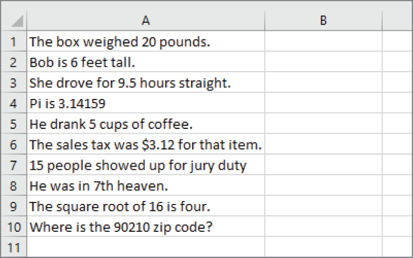
FIGURE 22.13 The goal is to extract the numbers from column A.
To try using Flash Fill, select cell B1 and type the first number (20). Move to B2 and type the second number (6). Can Flash Fill identify the remaining numbers and fill them in? Choose Data ➪ Data Tools ➪ Flash Fill (or press Ctrl+E), and Excel fills in the remaining cells in a flash. Figure 22.14 shows the result.
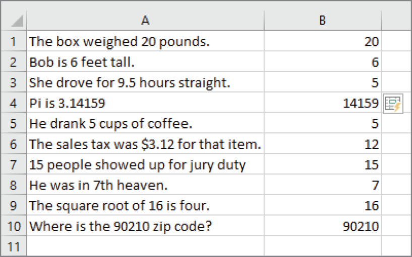
FIGURE 22.14 Using manually entered examples in B1 and B2, Excel's Flash Fill feature makes some incorrect guesses.
As you can see, Excel identified most of the values. Accuracy increases if you provide more examples. For example, provide a decimal number. Delete the suggested values in column B, enter 3.12 in cell B6, and press Ctrl+E. This time, Flash Fill gets all of them correct (see Figure 22.15).
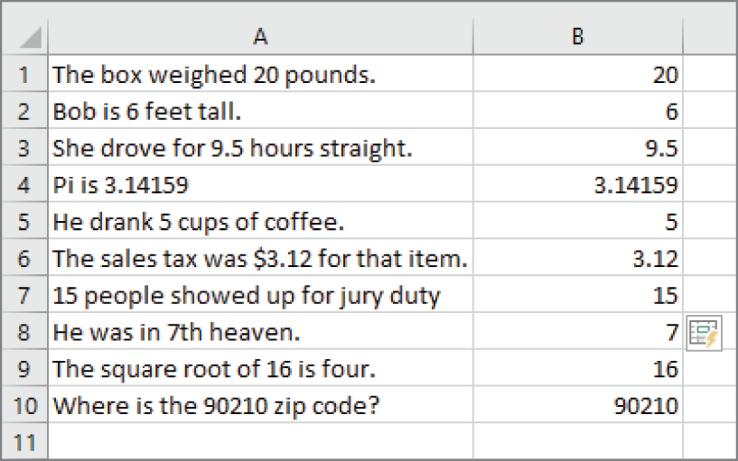
FIGURE 22.15 After you enter an example of a decimal number, Excel gets all of the values correct.
This simple example demonstrates two important points:
s- You must examine your data carefully after using Flash Fill. Just because the first few rows are correct, you can't assume that Flash Fill worked correctly for all rows.
- Flash Fill accuracy increases when you provide more examples.
Figure 22.16 shows another example: names in column A. The goal is to extract the first, last, and middle names (if it has one). In column B, Flash Fill successfully gets all the first names using only two examples (Mark and Tim). Plus, it successfully extracted all the last names (column C) using Russell and Colman. Extracting the middle names or initials (column D) didn't work until examples that included a space on either side of the middle name were included.
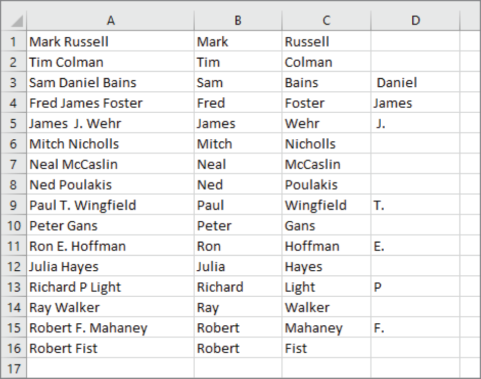
FIGURE 22.16 Using Flash Fill to split names
To summarize, Excel's Flash Fill is an interesting idea, but it works reliably only if the data is consistent. Even when you think it worked correctly, make sure that you examine the results carefully. And think twice before trusting it with important data because there's no way to document the way the data was extracted. But the main limitation is that (unlike formulas) Flash Fill is not a dynamic technique. If your data changes, the flash-filled columns do not update.
Changing the case of text
Often, you'll want to make text in a column consistent in terms of case. Excel provides no direct way to change the case of text, but it's easy to do with formulas. (See the sidebar “Transforming Data with Formulas.”)
The three relevant functions are as follows:
UPPER: This converts the text to ALL UPPERCASE.LOWER: This converts the text to all lowercase.PROPER: This converts the text to Proper Case. (The first letter in each word is capitalized, as in a proper name.)
These functions are quite straightforward. They operate only on alphabetic characters and just ignore all other characters and return them unchanged.
If you use the PROPER function, you'll probably need to do some additional cleanup to handle exceptions. The following are examples of transformations that you probably would consider incorrect:
- The letter following an apostrophe is always capitalized (for example, Don'T). This is done, apparently, to handle names like O'Reilly.
- The
PROPERfunction doesn't handle names with an embedded capital letter, such as McDonald. - “Minor” words such as and as well as the are always capitalized. For example, some people would prefer that the third word in United States Of America not be capitalized.
You can correct some of these problems by using Find and Replace.
Removing extra spaces
It's usually a good idea to ensure that data doesn't have extra spaces. It's difficult to spot a space character at the end of a text string. Extra spaces can cause lots of problems, especially when you need to compare text strings. The text July is not the same as the text July with a space appended to the end. The first is four characters long, and the second is five characters long.
The TRIM function removes all leading and trailing spaces and replaces interior multiple spaces with a single space. This formula uses the TRIM function. The formula returns Fourth Quarter Earnings (with no excess spaces):
=TRIM(" Fourth Quarter Earnings ")Data that is imported from a web page often contains a different type of space: a nonbreaking space, indicated by   in HTML code. In Excel, this character can be generated by this formula:
=CHAR(160)You can use a formula like this to replace those spaces with normal spaces:
=SUBSTITUTE(A2,CHAR(160)," ")Or you can use this formula to replace the nonbreaking space character with normal spaces and to remove excess spaces:
=TRIM(SUBSTITUTE(A2,CHAR(160)," "))Removing strange characters
Often, data imported into an Excel worksheet contains strange (sometimes unprintable) characters. You can use the CLEAN function to remove all nonprinting characters from a string. If the data is in cell A2, this formula will do the job:
=CLEAN(A2)Converting values
In some cases, you may need to convert values from one system to another. For example, you may import a file that has values in fluid ounces and they need to be expressed in milliliters. Excel's handy CONVERT function can perform that and many other conversions.
If cell A2 contains a value in ounces, the following formula converts it to milliliters:
=CONVERT(A2,"oz","ml")This function is extremely versatile and can handle most common measurement units in the following categories: weight and mass, distance, time, pressure, force, energy, power, magnetism, temperature, volume, liquid, area, bits and bytes, and speed.
Excel can also convert between number bases. You may import a file that contains hexadecimal values, and you need to convert them to decimal. Use the HEX2DEC function to perform this conversion. For example, the following formula returns 1,279, the decimal equivalent of its hex argument:
=HEX2DEC("4FF")Excel can also convert from binary to decimal (BIN2DEC) and from octal to decimal (OCT2DEC).
Functions that convert from decimal to another number base are DEC2HEX, DEC2BIN, and DEC2OCT and can be found in the Engineering category.
The BASE function converts a decimal number to any number base. Note that there is not a function that works in the opposite direction. Excel does not provide a function that converts any number base to decimal. You're limited to binary, octal, and hexadecimal.
Classifying values
Often, you may have values that need to be classified into a group. For example, if you have ages of people, you might want to classify them into groups such as 17 or younger, 18–24, 25–34, and so on.
The easiest way to perform this classification is with a lookup table. Figure 22.17 shows ages in column A and classifications in column B. Column B uses the lookup table in D2:E9. The formula in cell B2 is as follows:
=VLOOKUP(A2,$D$2:$E$9,2) 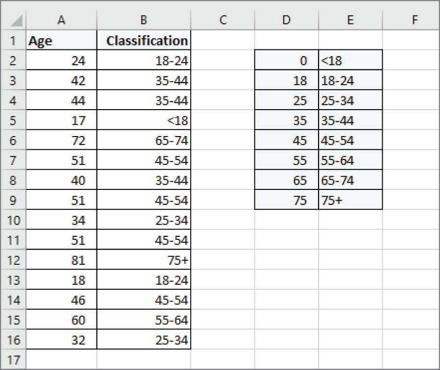
FIGURE 22.17 Using a lookup table to classify ages into age ranges
This formula was copied to the cells below.
You can also use a lookup table for nonnumeric data. Figure 22.18 shows a lookup table that is used to assign a region to a state.
The two-column lookup table is in the range D2:E52. The formula in cell B2, which was copied to the cells below, is as follows:
=VLOOKUP(A2,$D$2:$E$52,2,FALSE)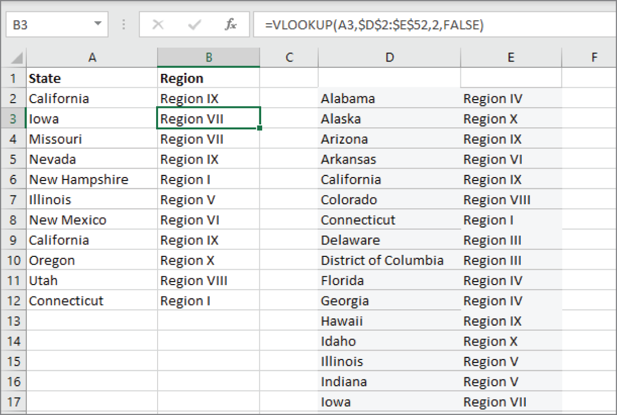
FIGURE 22.18 Using a lookup table to assign a region for a state
Joining columns
To combine data from two or more columns, you can use the CONCAT function in a formula. For example, the following formula combines the contents of cells A1, B1, and C1:
=CONCAT(A1:C1)Often, you'll need to insert spaces, or some other delimiter, between the cells—for example, if the columns contain a title, first name, and last name. Concatenating using the previous formulas would produce something like Mr.ThomasJones. To add spaces (to produce Mr. Thomas Jones), use the TEXTJOIN function:
=TEXTJOIN(" ",TRUE,A1:C1)The first argument of TEXTJOIN is the delimiter that you want to insert between the cell values. The second argument is TRUE to ignore empty cells. If you set the second argument to FALSE and there are empty cells, you'll end up with two delimiters right next to each other.
Figure 22.19 shows three examples of TEXTJOIN. In the first example, there are no empty cells, so the second argument doesn't matter. In the second and third examples, the second argument is set to FALSE and TRUE, respectively, and the delimiter is changed from a space to a comma (so it's easier to see the duplication). Where empty cells are not ignored, two commas are shown together.
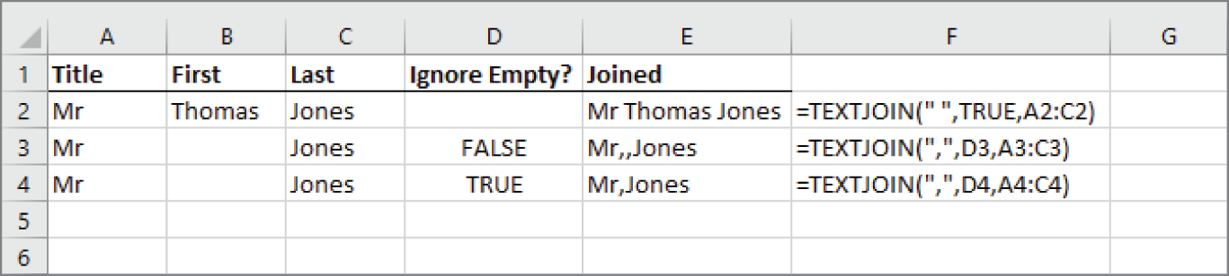
FIGURE 22.19 The TEXTJOIN function inserts delimiters between cell values.
You can also use the Flash Fill feature (discussed earlier in this chapter) to join columns without using formulas. Just provide an example or two in an adjacent column and press Ctrl+E. Excel will perform the concatenation for the other rows.
Rearranging columns
If you need to rearrange the columns in a worksheet, you could insert a blank column and then drag another column into the new blank column. But the moved column leaves a gap, which you need to delete.
Here's an easier way:
- Click the column header of the column you want to move.
- Choose Home ➪ Clipboard ➪ Cut.
- Click the column header to the right of where you want the column to go.
- Right-click and choose Insert Cut Cells from the shortcut menu.
Repeat these steps until the columns are in the order you want.
Randomizing the rows
If you need to arrange the rows in random order, here's a quick way to do it. In the column to the right of the data, insert this formula into the first cell and copy it down:
=RAND()Then sort the data using this column as the sort key. The rows will be in random order, and you can delete the column.
Extracting a filename from a URL
In some cases, you may have a list of URLs and need to extract only the filename. The following formula returns the filename from a URL. Assume that cell A2 contains this URL:
http://example.com/assets/images/horse.jpgThe following formula returns horse.jpg
:
=RIGHT(A2,LEN(A2)-FIND("*",SUBSTITUTE(A2,"/","*",LEN(A2)-LEN(SUBSTITUTE(A2,"/","")))))
This formula returns all text that follows the last slash character. If cell A2 doesn't contain a slash character, the formula returns an error.
To extract the URL without the filename, use this formula:
=LEFT(A2,FIND("*",SUBSTITUTE(A2,"/","*",LEN(A2)-LEN(SUBSTITUTE(A2,"/","")))))
Matching text in a list
You may have some data that you need to check against another list. For example, you may want to identify the data rows in which data in a particular column appears in a different list. Figure 22.20 shows a simple example. The data is in columns A:C. The goal is to identify the rows in which the Member Num appears in the Resigned Members list in column F. These rows can then be deleted.
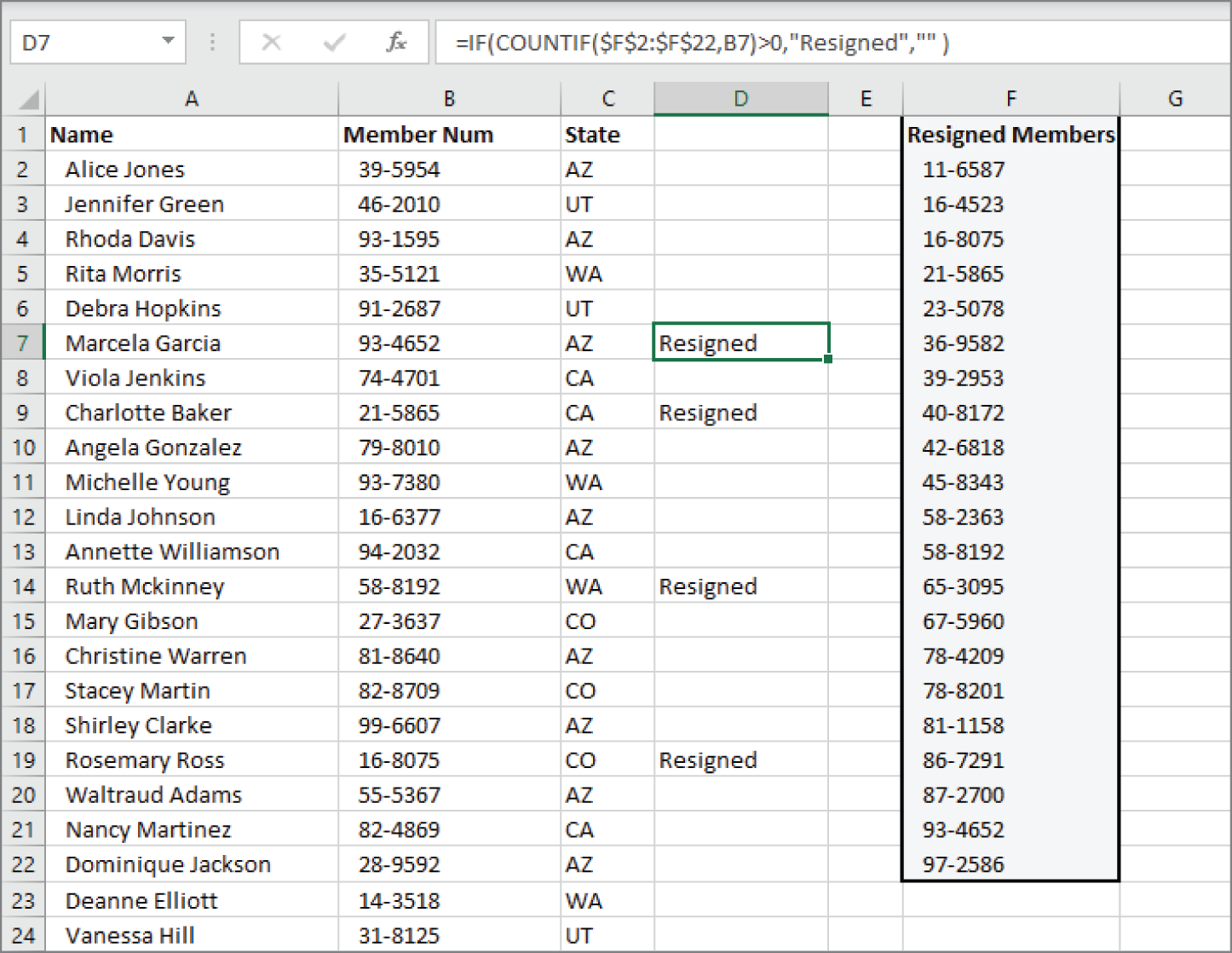
FIGURE 22.20 The goal is to identify member numbers that are in the Resigned Members list in column F.
Here's a formula, entered into cell D2 and copied down, that will do the job:
=IF(COUNTIF($F$2:$F$22,B2)>0,"Resigned","")This formula displays the word Resigned if the member number in column B is found in the Resigned Members list. If the member number is not found, it returns an empty string. If the list is sorted by column D, the rows for all resigned members will appear together and can be quickly deleted.
This technique can be adapted to other types of list-matching tasks.
Changing vertical data to horizontal data
Figure 22.21 shows a common type of data layout that you might see when importing a file. Each record consists of three consecutive cells in a single column: Name, Department, and Location. The goal is to convert this data so that each record appears in three columns.
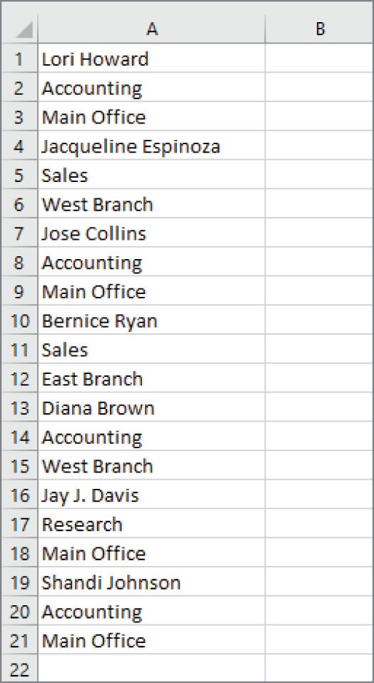
FIGURE 22.21 Vertical data that needs to be converted to three columns
There are several ways to convert this type of data, but here's a method that's fairly easy. It requires a small amount of setup, but the work is done with a single formula, which is copied to a range.
Start by creating some numeric vertical and horizontal “headers,” as shown in Figure 22.22. Column C contains numbers that correspond to the first row of each data item (in this case, the name). In this example, we put the following values in column C: 1, 4, 7, 10, 13, 16, and 19. You can use a simple formula to generate this series of numbers.
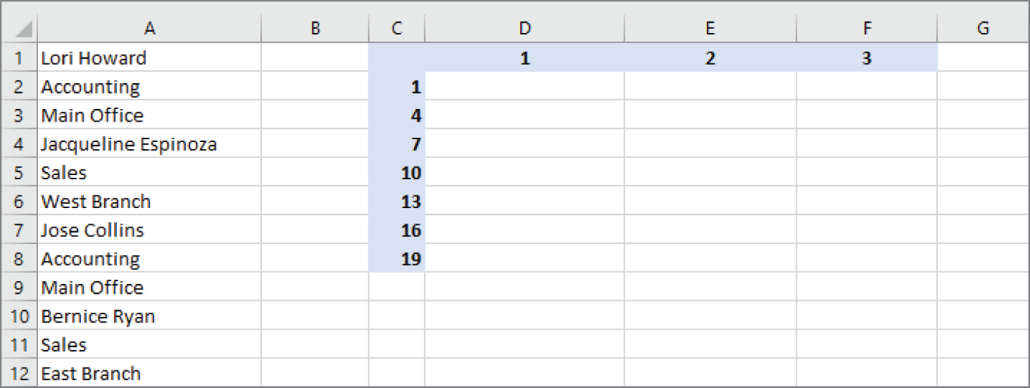
FIGURE 22.22 Headers that are used to convert the vertical data into rows
The horizontal range of headers consists of consecutive integers, starting with 1. In this example, each record contains three cells of data, so the horizontal header contains 1, 2, and 3.
Here's the formula that goes into cell D2:
=OFFSET($A$1,$C2+D$1-2,0)Copy this formula across to the next two columns and down to the next six rows. The result is shown in Figure 22.23.
You can easily adapt this technique to work with vertical data that contains a different number of rows. For example, if each record contained 10 rows of data, the column C header values would be 1, 11, 21, 31, and so on. The horizontal headers would consist of values 1 through 10 rather than 1 through 3.
Notice that the formula uses an absolute reference to cell A1. That reference won't change when the formula is copied, so all the formulas use cell A1 as the base. If the data begins in a different cell, change $A$1 to the address of the first cell.
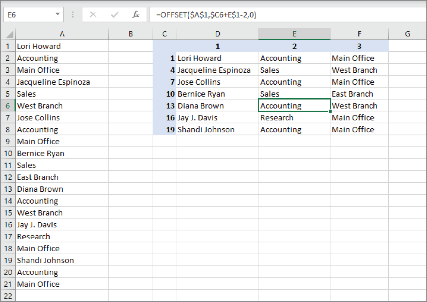
FIGURE 22.23 A single formula transforms the vertical data into rows.
The formula also uses “mixed” referencing in the second argument of the OFFSET function. The C2 reference has a dollar sign in front of C, so column C is the absolute part of the reference. In the D1 reference, the dollar sign is before the 1, so row 1 is the absolute part of the reference.
Filling gaps in an imported report
When you import data, you can sometimes end up with a worksheet that looks something like the one shown in Figure 22.24. This type of report formatting is common. As you can see, an entry in column A applies to several rows of data. If you sort this type of list, the missing data messes things up, and you can no longer tell who sold what when.
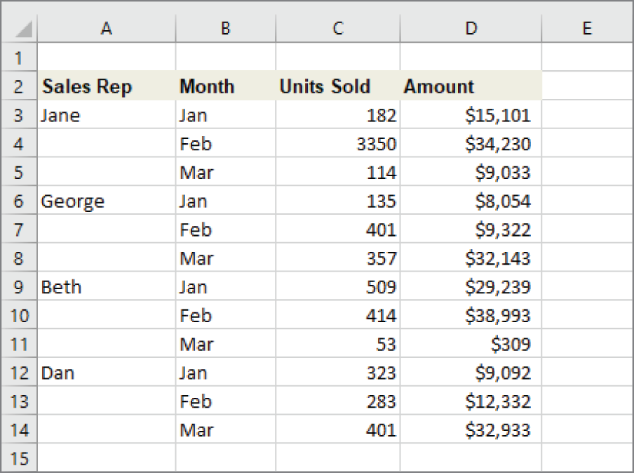
FIGURE 22.24 This report contains gaps in the Sales Rep column.
If the report is small, you can enter the missing cell values manually or by using a series of Home ➪ Editing ➪ Fill ➪ Down commands (or the Ctrl+D shortcut). But if you have a large list that's in this format, here's a better way:
- Select the range that has the gaps (
A3:A14, in this example). - Choose Home ➪ Editing ➪ Find & Select ➪ Go To Special. The Go To Special dialog box appears.
- Select the Blanks option and click OK. This action selects the blank cells in the original selection.
- In the formula bar, type an equal sign (
=) followed by the address of the first cell with an entry in the column (=A3, in this example) and press Ctrl+Enter. - Reselect the original range and press Ctrl+C to copy the selection.
- Choose Home ➪ Clipboard ➪ Paste ➪ Paste Values to convert the formulas to values.
After you complete these steps, the gaps are filled in with the correct information, and your worksheet looks similar to the one shown in Figure 22.25.
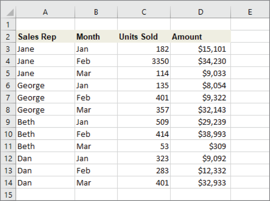
FIGURE 22.25 The gaps are gone, and this list can now be sorted.
Checking spelling
If you use a word-processing program, you probably take advantage of its spell-checker feature. Spelling mistakes can be embarrassing when they appear in a text document, but they can cause serious problems when they occur within your data. For example, if you tabulate data by month, a misspelled month name will make it appear that a year has 13 months.
To access the Excel spell-checker, choose Review ➪ Proofing ➪ Spelling, or press F7. To check the spelling in just a particular range, select the range before you activate the spell-checker.
If the spell-checker finds any words it doesn't recognize as correct, it displays the Spelling dialog box. The options are fairly self-explanatory.
Replacing or removing text in cells
You may need to replace (or remove) certain characters systematically in a column of data. For example, you may need to replace all backslash characters with forward slash characters. In many cases, you can use Excel's Find and Replace dialog box to accomplish this task. To remove text using the Find and Replace dialog box, just leave the Replace With field empty.
In other situations, you may need a formula-based solution. Consider the data shown in Figure 22.26. The goal is to replace the second hyphen character with a colon for the part numbers in column A. Using Find and Replace wouldn't work because there isn't a way to specify that only the second hyphen should be replaced.
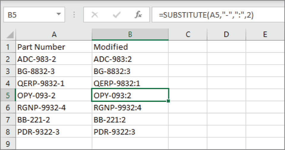
FIGURE 22.26 To replace only the second hyphen in these cells, Find and Replace is not an option.
In this case, the solution is a fairly simple formula that replaces the second occurrence of a hyphen with a colon:
=SUBSTITUTE(A2,"-",":",2)To remove the second occurrence of a hyphen, just omit the third argument for the SUBSTITUTE function:
=SUBSTITUTE(A2,"-",,2)This is another example where Flash Fill can also do the job.
Adding text to cells
If you need to add text to a cell, one solution is to use a new column of formulas. Here are some examples:
- The following formula adds
ID:and a space to the beginning of a cell:
-
="ID: "&A2
- The following formula adds
.mp3to the end of a cell:
-
=A2&".mp3"
- The following formula inserts a hyphen after the third character in a cell:
-
=LEFT(A2,3)&"-"&RIGHT(A2,LEN(A2)-3)
You can also use the Flash Fill feature to add text to cells.
Fixing trailing minus signs
Imported data sometimes displays negative values with a trailing minus sign. For example, a negative value may appear as 3,498– rather than the more common –3,498. Excel does not convert these values. In fact, it considers them to be nonnumeric text.
The solution is so simple it may even surprise you:
- Select the data that has the trailing minus signs. The selection can also include positive values.
- Choose Data ➪ Data Tools ➪ Text to Columns. The Text to Columns dialog box appears.
- Click Finish.
This procedure works because of a default setting in the Advanced Text Import Settings dialog box (which you don't even see normally). To display this dialog box, which is shown in Figure 22.27, go to step 3 in the Text to Columns Wizard dialog box and click Advanced.
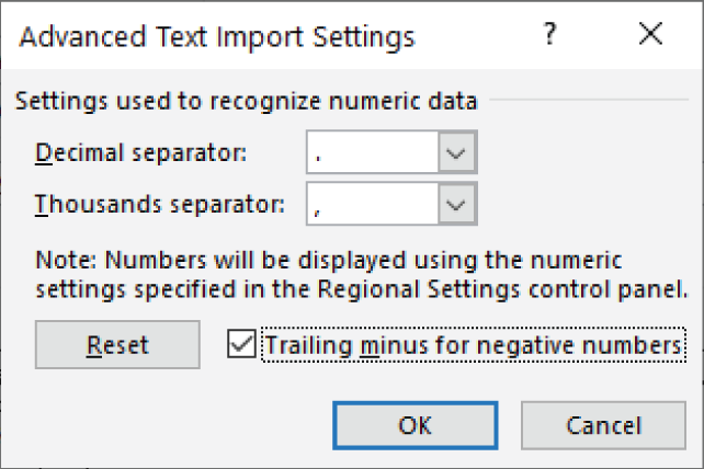
FIGURE 22.27 The Trailing Minus for Negative Numbers option makes it easy to fix trailing minus signs in a range of data.
Following a data cleaning checklist
This section contains a list of items that could cause problems with data. Not all of these are relevant to every set of data.
- Does each column have a unique and descriptive header?
- Is each column of data formatted consistently?
- Did you check for duplicate or missing rows?
- For text data, are the words consistent in terms of case?
- Did you check for spelling errors?
- Does the data contain any extra spaces?
- Are the columns arranged in the proper (or logical) order?
- Are there any blank cells that shouldn't be blank?
- Did you correct any trailing minus signs?
- Are the columns wide enough to display all data?
Exporting Data
This chapter began with sections on importing data, so it's only appropriate to end it with a discussion of exporting data to a file that's not a standard Excel file.
Exporting to a text file
When you choose File ➪ Save As, the Save As dialog box lets you choose from a variety of file formats. The three text file types are as follows:
- CSV: Comma-separated value files
- TXT: Tab-delimited files
- PRN: Formatted text
We discuss these file types in the sections that follow.
CSV files
When you export a worksheet to a CSV file, the data is saved as displayed. In other words, if a cell contains 12.8312344 but is formatted to display with two decimal places, the value will be saved as 12.83.
Cells are delimited with a comma character, and rows are delimited with a carriage return and line feed.
Note that if a cell contains a comma, the cell value is saved within quotation marks. If a cell contains a quotation mark character, that character appears twice.
TXT files
Exporting a workbook to a TXT file is almost identical to the CSV file format described earlier. The only difference is that cells are separated by a tab character rather than a comma.
If your worksheet contains any Unicode characters, you should export the file using the Unicode variant. Otherwise, Unicode characters will be saved as question mark characters.
PRN files
A PRN file is very much like a printed image of the worksheet. The cells are separated by multiple space characters. Also, a line is limited to 240 characters. If a line exceeds that limit, the remainder appears on the next line. PRN files are rarely used.
Exporting to other file formats
Excel also lets you save your work in several other formats:
- Data Interchange Format These files have a
.diffilename extension. These are not used very often. - Symbolic Link These files have an
.slk filenameextension. These are not used very often. - Portable Document Format These files have a
.pdffilename extension. This is a common “read-only” file format. - XML Paper Specification Document These files have an
.xpsfilename extension. This is Microsoft's alternative to PDF files. It is not used very often. - Web Page These files have an
.htmfilename extension. Often, saving a file as a webpage will generate a directory of ancillary files required to render the page accurately. - OpenDocument Spreadsheet These files have an
.odsfilename extension. They're compatible with various open-source spreadsheet programs.