
CHAPTER 13
Using Formulas with Dates and Times
Many worksheets contain dates and times in cells. For example, you might track information by date or create a schedule based on time. Beginners often find that working with dates and times in Excel can be frustrating. To work with dates and times, you need a good understanding of how Excel handles time-based information. This chapter provides the information you need to create powerful formulas that manipulate dates and times.
Understanding How Excel Handles Dates and Times
The following sections present a quick overview of how Excel deals with dates and times. It covers Excel's date and time serial number system. It also provides some tips for entering and formatting dates and times.
Understanding date serial numbers
To Excel, a date is simply a number. More precisely, a date is a serial number that represents the number of days since the fictitious date of January 0, 1900. A serial number of 1 corresponds to January 1, 1900; a serial number of 2 corresponds to January 2, 1900; and so on. This system makes it possible to create formulas that perform calculations with dates. For example, you can create a formula to calculate the number of days between two dates (just subtract one from the other).
Excel supports dates from January 1, 1900, through December 31, 9999 (serial number = 2958465).
You may wonder about January 0, 1900. This nondate (which corresponds to date serial number 0) is actually used to represent times that aren't associated with a particular day. This concept becomes clear later in this chapter. (See “Entering times.”)
To view a date serial number as a date, you must format the cell as a date. Choose Home ➪ Number ➪ Number Format. This drop-down control provides you with two date formats. To select from additional date formats, see “Formatting dates and times” later in this chapter.
Entering dates
You can enter a date directly as a serial number (if you know the serial number) and then format it as a date. More often, you enter a date by using any of several recognized date formats. Excel automatically converts your entry into the corresponding date serial number (which it uses for calculations), and it applies the default date format to the cell so that it displays as an actual date rather than as a cryptic serial number.
For example, if you need to enter June 18, 2022, into a cell, you can enter the date by typing June 18, 2022 (or any of several different date formats). Excel interprets your entry and stores the value 44730, the date serial number for that date. It also applies the default date format, so the cell contents may not appear exactly as you typed them.
When you activate a cell that contains a date, the Formula bar shows the cell contents formatted by using the default date format—which corresponds to your system's short date format. The Formula bar doesn't display the date's serial number. If you need to find out the serial number for a particular date, format the cell with the General format.
Excel is rather flexible when it comes to recognizing dates entered into a cell. It's not perfect, however. If you attempt to enter a date that lies outside the supported date range, Excel interprets it as text. If you attempt to format a serial number that lies outside the supported range as a date, the value displays as a series of hash marks (#########).
Understanding time serial numbers
When you need to work with time values, you extend the Excel date serial number system to include decimals. In other words, Excel works with time by using fractional days. For example, the date serial number for June 1, 2022, is 44713. Noon (halfway through the day) is represented internally as 44713.5.
The serial number equivalent of one minute is approximately 0.00069444. The following formula calculates this number by multiplying 24 hours by 60 minutes and dividing the result into 1. The denominator consists of the number of minutes in a day (1,440).
=1/(24*60)Similarly, the serial number equivalent of one second is approximately 0.00001157, obtained by the following formula:
=1/(24*60*60)In this case, the denominator represents the number of seconds in a day (86,400).
In Excel, the smallest unit of time is one 1,000th of a second. The time serial number shown here represents 23:59:59.999 (one 1,000th of a second before midnight):
0.99999999Table 13.1 shows various times of day along with each associated time serial number.
TABLE 13.1 Times of Day and Their Corresponding Serial Numbers
| Time of Day | Time Serial Number |
|---|---|
| 12:00:00 AM (midnight) | 0.00000000 |
| 1:30:00 AM | 0.06250000 |
| 7:30:00 AM | 0.31250000 |
| 10:30:00 AM | 0.43750000 |
| 12:00:00 PM (noon) | 0.50000000 |
| 1:30:00 PM | 0.56250000 |
| 4:30:00 PM | 0.68750000 |
| 6:00:00 PM | 0.75000000 |
| 9:00:00 PM | 0.87500000 |
| 10:30:00 PM | 0.93750000 |
Entering times
As with entering dates, you normally don't have to worry about the actual time serial numbers. Just enter the time into a cell using a recognized format. Table 13.2 shows some examples of time formats that Excel recognizes.
TABLE 13.2 Time Entry Formats Recognized by Excel
| Entry | Excel Interpretation |
|---|---|
| 11:30 AM | 11:30 AM |
| 11:30:00 AM | 11:30 AM |
| 11:30 PM | 11:30 PM |
| 11:30 | 11:30 AM |
| 13:30 | 1:30 PM |
Because the preceding samples don't have a specific day associated with them, Excel uses a date serial number of 0, which corresponds to the nonday January 0, 1900. Often, you'll want to combine a date and time. Do so by using a recognized date entry format, followed by a space, and then a recognized time entry format. For example, if you enter 6/1/2022 11:30 into a cell, Excel interprets it as 11:30 AM on June 1, 2022. Its date/time serial number is 44713.47917.
When you enter a time that exceeds 24 hours, the associated date for the time increments accordingly. For example, if you enter 25:00:00 into a cell, it's interpreted as 1:00 AM on January 1, 1900. The day part of the entry increments because the time exceeds 24 hours. Keep in mind that a time value without a date uses January 0, 1900, as the date.
Similarly, if you enter a date and a time (and the time exceeds 24 hours), the date you entered is adjusted. If you enter 9/18/2022 25:00:00, for example, it's interpreted as 9/19/2022 1:00:00 AM.
If you enter a time only (without an associated date) into an unformatted cell, the maximum time you can enter into a cell is 9999:59:59 (just less than 10,000 hours). Excel adds the appropriate number of days. In this case, 9999:59:59 is interpreted as 3:59:59 PM on 02/19/1901. If you enter a time that exceeds 10,000 hours, the entry is interpreted as a text string rather than a time.
Formatting dates and times
You have a great deal of flexibility in formatting cells that contain dates and times. For example, you can format the cell to display the date part only, the time part only, or both the date and time parts.
You format dates and times by selecting the cells and then using the Number tab of the Format Cells dialog box. To display this dialog box, click the dialog box launcher icon in the Number group of the Home tab, or click the Number Format control and choose More Number Formats from the list that appears.
The Date category shows built-in date formats, and the Time category shows built-in time formats. Some formats include both date and time displays. Just select the desired format from the Type list and then click OK.
Problems with dates
Excel has some problems when it comes to dates. Many of these problems stem from the fact that Excel was designed many years ago. Excel designers basically emulated the Lotus 1-2-3 program's limited date and time features, which contain a nasty bug that was duplicated intentionally in Excel (described next). If Excel were being designed from scratch today, I'm sure it would be much more versatile in dealing with dates. Unfortunately, users are currently stuck with a product that leaves much to be desired in the area of dates.
Excel's leap year bug
A leap year, which occurs every four years, contains an additional day (February 29). Specifically, years that are evenly divisible by 100 are not leap years, unless they are also evenly divisible by 400. Although the year 1900 was not a leap year, Excel treats it as such. In other words, when you type 2/29/1900 into a cell, Excel interprets it as a valid date and assigns a serial number of 60.
If you type 2/29/1901, however, Excel correctly interprets it as a mistake and doesn't convert it to a date. Instead, it simply makes the cell entry a text string.
How can a product used daily by millions of people contain such an obvious bug? The answer is historical. The original version of Lotus 1-2-3 contained a bug that caused it to treat 1900 as a leap year. When Excel was released some time later, the designers knew about this bug and chose to reproduce it in Excel to maintain compatibility with Lotus 1-2-3 worksheet files.
Why does this bug still exist in later versions of Excel? Microsoft asserts that the disadvantages of correcting this bug outweigh the advantages. If the bug were eliminated, it would mess up millions of existing workbooks. In addition, correcting this problem would possibly affect compatibility between Excel and other programs that use dates. As it stands, this bug really causes very few problems because most users don't use dates prior to March 1, 1900.
Pre-1900 dates
The world, of course, didn't begin on January 1, 1900. People who use Excel to work with historical information often need to work with dates before January 1, 1900. Unfortunately, the only way to work with pre-1900 dates is to enter the date into a cell as text. For example, you can enter July 4, 1776, into a cell, and Excel won't complain.
Using text as dates works in some situations, but the main problem is that you can't perform manipulation on a date that's entered as text. For example, you can't change its numeric formatting, you can't determine which day of the week this date occurred, and you can't calculate the date that occurs seven days later.
Inconsistent date entries
You need to be careful when entering dates by using two digits for the year. When you do so, Excel has some rules that determine which century to use.
Two-digit years between 00 and 29 are interpreted as 21st-century dates, and two-digit years between 30 and 99 are interpreted as 20th-century dates. For example, if you enter 12/15/28, Excel interprets your entry as December 15, 2028. But if you enter 12/15/30, Excel sees it as December 15, 1930, because Windows uses a default boundary year of 2029. You can keep the default as is or change it via the Windows Control Panel. From the Region dialog box, click the Additional Settings button to display the Customize Format dialog box. Select the Date tab and then specify a different year.
Using Excel's Date and Time Functions
Excel has quite a few functions that work with dates and times. These functions are accessible by choosing Formulas ➪ Function Library ➪ Date & Time.
These functions leverage the fact that, beneath the covers, dates and times are nothing more than a numbering system. This opens the door for all kinds of cool formula-driven analyses. In the following sections, you'll walk through some of these cool analyses. Along the way, you'll pick up a few techniques that will help you create your own formulas.
Getting the current date and time
Instead of typing the current date and time, you can use one of two Excel functions. The TODAY function returns the current date:
=TODAY()The NOW() function returns the current date along with the current time:
=NOW()Both the TODAY and NOW functions return date serial numbers that represent the current system date and time. The TODAY function assumes 12:00 AM as the time, while the NOW function returns the actual time.
It's important to note that both of these functions will automatically recalculate each time you change or open your workbook, so don't use these functions as a timestamp of record.
You can use the TODAY function as part of a text string by wrapping it in the TEXT function with some date formatting. This formula will display text that will return today's date in Month Day, Year format.
="Today is "&TEXT(TODAY(),"mmmm d, yyyy")Calculating age
One of the easiest ways to calculate the age of anything is to use Excel's DATEDIF function. This function makes calculating any kind of date comparisons a breeze.
To calculate a person's age using the DATEDIF function, you can enter a formula like this:
=DATEDIF("5/16/1972",TODAY(),"y")You can, of course, reference a cell that contains a date:
=DATEDIF(B4,TODAY(),"y")The DATEDIF function calculates the number of days, months, or years between two dates. It requires three arguments—a start date, an end date, and a time unit.
The time units are defined by a series of codes listed in Table 13.3.
TABLE 13.3 DATEDIF Time Unit Codes
| Code | What It Returns |
|---|---|
"y"
| The number of complete years in the period. |
"m"
| The number of complete months in the period. |
"d"
| The number of days in the period. |
"md"
| The difference between the days in start_date and end_date. The months and years of the dates are ignored. |
"ym"
| The difference between the months in start_date and end_date. The days and years of the dates are ignored. |
"yd"
| The difference between the days of start_date and end_date. The years of the dates are ignored. |
Using these time codes, you can easily calculate the number of years, months, and days between two dates. If someone was born on May 16, 1972, you could find that person's age in years, months, and days using these respective formulas:
=DATEDIF("5/16/1972",TODAY(),"y")=DATEDIF("5/16/1972",TODAY(),"m")=DATEDIF("5/16/1972",TODAY(),"d")
Calculating the number of days between two dates
One of the most common date calculations performed in the corporate world is figuring the number of days between two dates. Project management teams use it to measure performance against a milestone, HR departments use it to measure time to fill a requisition, and finance departments use it to track aging receivables. Luckily, it's one of the easiest calculations to perform thanks to the handy DATEDIF function.
Figure 13.1 demonstrates a sample report that uses the DATEDIF function to calculate the number of days outstanding for a set of invoices.
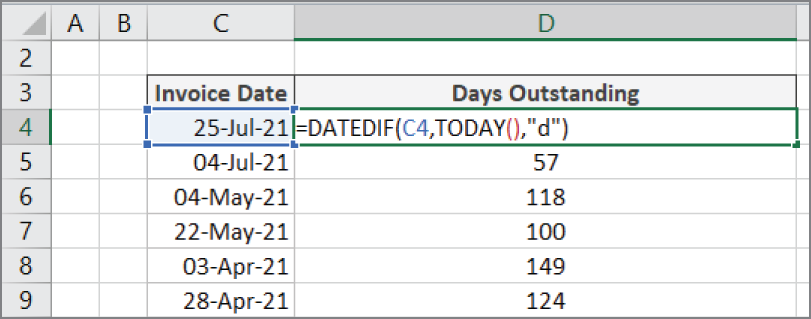
FIGURE 13.1 Calculating the number of days between today and the invoice date
Looking at Figure 13.1, you'll see the formula in cell D4 is as follows:
=DATEDIF(C4,TODAY(),"d")This formula uses the DATEDIF function with the time code d. This tells Excel to return the number of days based on the start date (C4) and the end date (TODAY).
Calculating the number of workdays between two dates
Oftentimes when reporting on the elapsed number of days between a start date and end date, it's not appropriate to count the weekends in the final number of days. Operations are typically shut down on the weekends, so you would want to avoid counting those days.
You can use Excel's NETWORKDAYS function to calculate the number of days between a start date and end date excluding weekends.
As you can see in Figure 13.2, the NETWORKDAYS function is used in cell E4 to calculate the number of workdays between 1/1/2022 and 12/31/2022.

FIGURE 13.2 Calculating the number of workdays between two dates
This formula is fairly straightforward. The NETWORKDAYS function has two required arguments: a start date and an end date. If your start date is in cell B4 and your end date is in cell C4, this formula would return the number of workdays (excluding Saturdays and Sundays):
=NETWORKDAYS(B4,C4)Using NETWORKDAYS.INTL
The one drawback to using the NETWORKDAYS function is that it defaults to excluding Saturday and Sunday. But what if you work in a region where the weekends are actually Fridays and Saturdays? Or worse yet, what if your weekends only include Sundays?
Excel has you covered with the NETWORKDAYS.INTL function. In addition to the required start and end dates, this function has an optional third argument—a weekend code. The weekend code allows you to specify which days to exclude as a weekend day.
As you enter the NETWORKDAYS.INTL function, Excel displays a menu as soon as you go into the third argument (see Figure 13.3). Simply select the appropriate weekend code and press Enter.
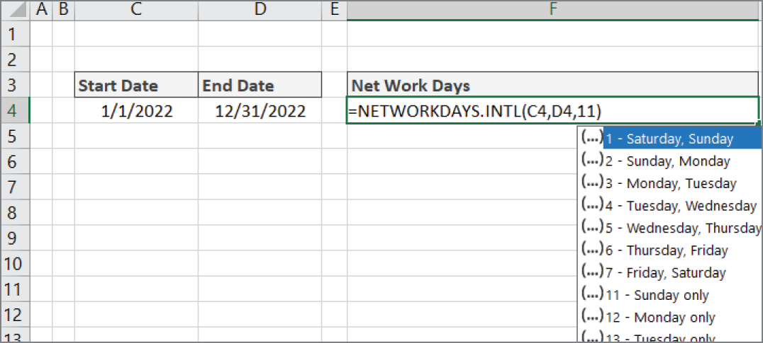
FIGURE 13.3 NETWORKDAY.INTL allows you to specify which days to exclude as weekend days.
Generating a list of business days excluding holidays
When creating dashboards and reports in Excel, it's often useful to have a helper table that contains a list of dates that represent business days (that is, dates that are not weekends or holidays). This kind of a helper table can help assist in calculations like revenue per business day, units per business day, and so on.
One of the easiest ways to generate a list of business days is to use the WORKDAY.INTL function. Start with a spreadsheet that contains the last date of the previous year and a list of your organization's holidays. As you can see in Figure 13.4, your list of holidays should be formatted as dates.
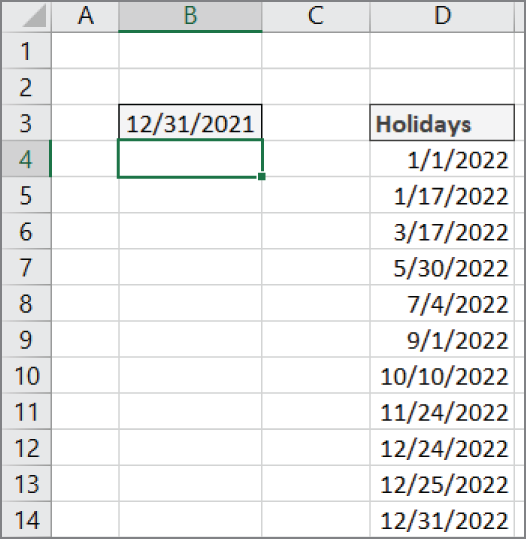
FIGURE 13.4 Start with a sheet containing the last date of the previous year and a list of holidays.
In the cell beneath the last date of the previous year, enter this formula:
=WORKDAY.INTL(B3,1,1,$D$4:$D$14)At this point, you can copy the formula down to create as many business days as you need (see Figure 13.5).
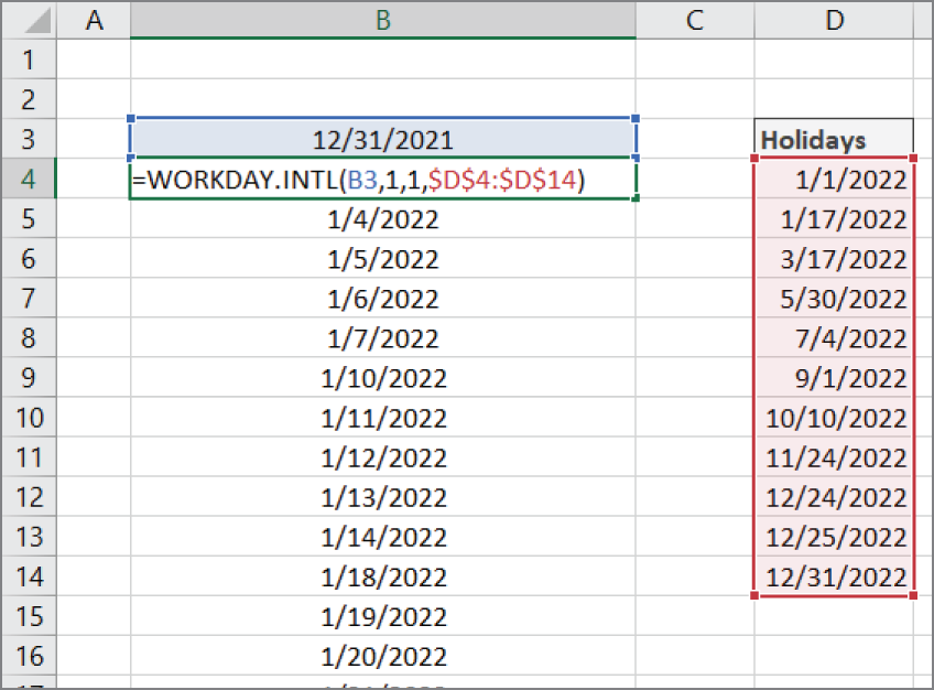
FIGURE 13.5 Creating a list of business days
The WORKDAY.INTL function returns a workday date based on the number of days you tell it to increment. This function has two required arguments and two optional arguments:
- Start Date (required) This argument is the date to start from.
- Days (required) This argument is the number of days from the start date that you want returned.
- Weekends (optional) By default, the
WORKDAY.INTLfunction excludes Saturdays and Sundays, but this third argument allows you to specify which weekdays to exclude as a weekend day. As you enter theWORKDAY.INTLfunction, Excel displays a menu where you can select the appropriate weekend code. - Holidays (optional) This argument allows you to give Excel a list of dates to exclude in addition to the weekend days.
In this example, we are telling Excel to start from 12/31/2021 and then increment up 1 to give us the next business day after our start date. For our optional arguments, we specify that we need to exclude Saturdays and Sundays, along with the holidays listed in cells $D$4:$D$14.
=WORKDAY.INTL(B3,1,1,$D$4:$D$14)Be sure to lock down the range for your list of holidays with absolute references so that it remains locked as you copy your formula down.
Extracting parts of a date
Although it may seem trivial, it's often helpful to pick out a specific part of a date. For example, you may need to filter all records that have order dates within a certain month or all employees who have time allocated to Saturdays. In these situations, you would need to pull out the month and workday number from the formatted dates.
Excel provides a simple set of functions to parse dates out into their component parts. These functions are as follows:
YEARextracts the year from a given date.MONTHextracts the month from a given date.DAYextracts the month day number from a given date.WEEKDAYreturns the weekday number for a given date.WEEKNUMreturns the week number for a given date.
Figure 13.6 demonstrates the use of these functions to parse the date in cell C3 into its component parts.
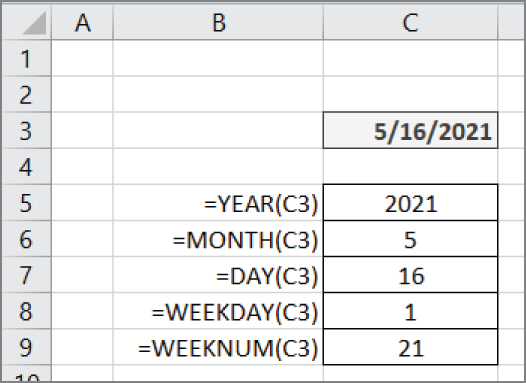
FIGURE 13.6 Extract the parts of a date.
These functions are fairly straightforward.
The YEAR function returns a four-digit number that corresponds to the year of a specified date. This formula returns 2021.
=YEAR("5/16/2021")The MONTH function returns a number between 1 and 12 that corresponds to the month of a specified date. This formula returns 5.
=MONTH("5/16/2021")The DAY function returns a number between 1 and 31 that corresponds to the day of the month represented in a specified date. This formula returns 16.
=DAY("5/16/2021")The WEEKDAY function returns a number from 1 to 7 that corresponds to the day of the week (Sunday through Saturday) on which the given date falls. If the date falls on a Sunday, the number 1 is returned. If the date falls on a Monday, the number 2 is returned, and so on. This formula returns 1 because 5/16/2021 falls on a Sunday.
=WEEKDAY("5/16/2021")This function actually has an optional return_type argument that lets you define which day of the week holds the first position. As you enter the WEEKDAY function, Excel displays a menu where you can select the appropriate return_type code.
You can adjust the formula so that the return values 1 through 7 represent Monday through Sunday.
=WEEKDAY("5/16/2021",2)The WEEKNUM function returns the week number in the year for the week in which the specified date occurs. This formula returns 21 because 5/16/2021 falls within week 21 in 2021.
=WEEKNUM("5/16/2021")This function actually has an optional return_type argument that lets you specify which day of the week defines the start of the week. By default, the WEEKNUM function defines the start of the week as Sunday. As you enter the WEEKNUM function, Excel displays a menu where you can select a different return_type code.
Calculating number of years and months between dates
In some cases, you'll be asked to express the difference between two dates in years and months. In these cases, you can create a text string using two DATEDIF functions.
Cell C4 shown in Figure 13.7 contains the following formula:
=DATEDIF(A4,B4,"Y") & " Years, " & DATEDIF(A4,B4,"YM") & " Months" We accomplish this task by using two DATEDIF functions joined in a text string with the ampersand (&) operator.
The first DATEDIF function calculates the number of years between the start and end dates by passing the year time unit (Y):
DATEDIF(A4,B4,"Y")The second DATEDIF function uses the YM time unit to calculate the number of months ignoring the year portion of the date:
DATEDIF(A4,B4,"YM")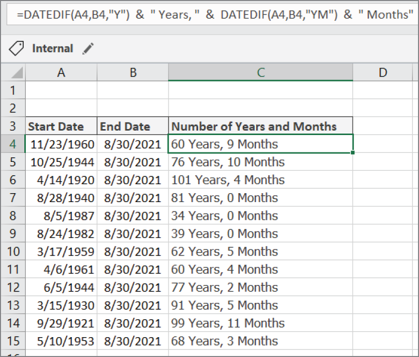
FIGURE 13.7 Showing the years and months between dates
We join these two functions with some text of our own to let the users know which number represents years and which represents months:
=DATEDIF(A4,B4,"Y") & " Years, " & DATEDIF(A4,B4,"YM") & " Months"Converting dates to Julian date formats
Julian dates are often used in manufacturing environments as a timestamp and quick reference for batch number. This type of date coding allows retailers, consumers, and service agents to identify when a product was made and thus the age of the product. Julian dates are also used in programming, the military, and astronomy.
Different industries have their own variations on Julian dates, but the most commonly used variation is made up of two parts: a two-digit number representing the year and the number of elapsed days in the year. For example, the Julian date for 1/1/1960 would be 601. The Julian date for 5/10/21 would be 21130.
Excel has no built-in function to convert a standard date to a Julian date, but Figure 13.8 illustrates how a formula can be used to accomplish the task.
=RIGHT(YEAR(A4),2)& A4-DATE(YEAR(A4),1,0) This formula is really two formulas joined as a text string using the ampersand (&).
The first formula uses the RIGHT function to extract the right two digits of the year number. Note we are using the YEAR function to pull out the year portion from the actual date.
=RIGHT(YEAR(A4),2)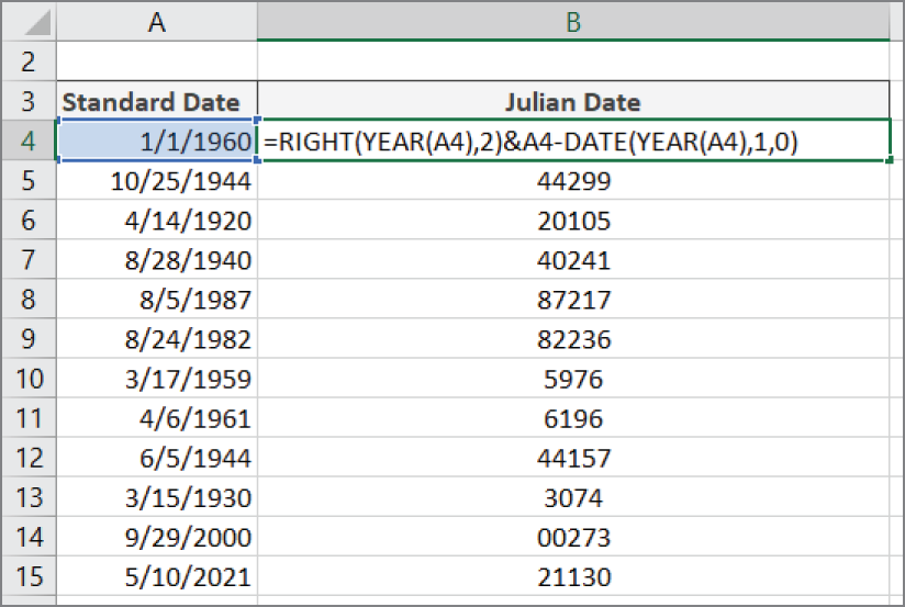
FIGURE 13.8 Converting standard dates into Julian dates
The second formula is a bit trickier. Here we have to find out how many days have elapsed since the beginning of the year. For this, we first need to subtract the target date from the last day of the previous year.
A4-DATE(YEAR(A4),1,0)You'll note the use of the DATE function. The DATE function allows us to build a date on the fly using three arguments: the year, the month, and the day. The year can be any whole number from 1900 to 9999. The month and date can be any positive or negative number. For example, this formula would return the date serial number for December 1, 2013:
=DATE(2013, 12, 1)Note that in our Julian date formula, we are using a zero as our day argument. When you use 0 as the day argument, you are telling Excel that you want the day before the 1st of the given month. In this example, the day before January 1 is December 31. For instance, entering this formula into a blank cell will return December 31, 1959:
=DATE(1960,1,0)Joining our two formulas together with an ampersand brings the Julian date together:
=RIGHT(YEAR(A4),2)&A4-DATE(YEAR(A4),1,0)Calculating the percent of year completed and remaining
When building Excel reports and dashboards, oftentimes it's beneficial to calculate the percent of the year that has elapsed and what percent remains. These percentages can be used in other calculations or simply as a notification for your audience.
Figure 13.9 shows a sample of this concept. Note in the Formula bar that we are using the YEARFRAC function.

FIGURE 13.9 Calculating the percent of the year completed
The YEARFRAC function simply requires a start date and an end date. Once it has those two variables, it calculates the fraction of the year representing the number of days between the start date and end date.
=YEARFRAC(B3,C3)To get the percent remaining, as shown in cell C7 of Figure 13.9, simply subtract 1 from the YEARFRAC formula:
=1-YEARFRAC(B3,C3)Returning the last date of a given month
A common need when working with dates is to calculate dynamically the last date in a given month. Although the last day for most months is fixed, the last day for February varies depending on whether the given year is a leap year.
Figure 13.10 illustrates how to get the last date in February for each date given in order to see which years are leap years.

FIGURE 13.10 Calculating the last day of each date
The DATE function lets you build a date on the fly using three arguments: the year, the month, and the day. The year can be any whole number from 1900 to 9999. The month and date can be any positive or negative number.
For example, this formula would return the date serial number for December 1, 2013:
=DATE(2013,12,1)When you use 0 as the day argument, you are telling Excel that you want the day before the 1st of the month. For instance, entering this formula into a blank cell will return February 29, 2000:
=DATE(2000,3,0)In our example, instead of hard-coding the year and month, we use the YEAR function to get the desired year and the MONTH function to get the desired month. We add 1 to the month so that we go into the next month. This way, when we use 0 as the day, we get the last day of the month in which we're actually interested.
=DATE(YEAR(B3),MONTH(B3)+1,0)As you look at Figure 13.10, keep in mind that you can use the formula to get the last day of any month, not just February.
Using the EOMONTH function
The EOMONTH function is an easy alternative to using the DATE function. With the EOMONTH function, you can get the last date of any future or past month. All you need is two arguments: a start date and the number of months in the future or past.
For example, this formula will return the last day of April 2022:
=EOMONTH("1/1/2022",3)Specifying a negative number of months will return a date in the past. This formula will return the last day of October 2021:
=EOMONTH("1/1/2022",-3)You can combine the EOMONTH function with the TODAY function to get the last day of the current month.
=EOMONTH(TODAY(),0)Calculating the calendar quarter for a date
Believe it or not, there is no built-in function to calculate quarter numbers in Excel. If you need to calculate into which calendar quarter a specific date falls, you'll need to create your own formula.
Figure 13.11 demonstrates the following formula used for calculating calendar quarters:
=ROUNDUP(MONTH(B3)/3,0) 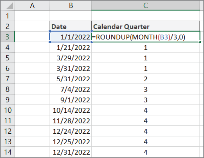
FIGURE 13.11 Calculating calendar quarters
The secret to this formula is simple math. Here you're dividing the month number for the given month by 3 and then rounding that number up to the nearest integer. For instance, let's say you want to calculate the quarter into which August falls. Since August is the 8th month of the year, you could divide 8 by 3. That would give you the answer 2.66. Round that number up, and you get 3. Thus, August is in the third quarter of the calendar year.
The following formula does the same thing. We're using the MONTH function to extract the month number from the given date and the ROUNDUP function to force rounding up.
=ROUNDUP(MONTH(B3)/3,0)Calculating the fiscal quarter for a date
Many of us work in organizations where the fiscal year does not start in January. Instead, it starts in October or April or any other month. In these organizations, the fiscal quarters can't be calculated in the same way as calendar quarters.
Figure 13.12 demonstrates a clever formula for converting a date into a fiscal quarter using the CHOOSE function. In this example, we're calculating the fiscal quarters when our fiscal year starts in April. The formula seen in the Formula bar shows the following:
=CHOOSE(MONTH(B3),4,4,4,1,1,1,2,2,2,3,3,3) The CHOOSE function returns an answer from a list of choices based on a position number. If you were to enter the formula =CHOOSE(2,"Gold","Silver","Bronze","Coupon"), you would get Silver because Silver is the second choice in your list of choices. Replace the 2 with a 4, and you would get Coupon, the fourth choice.

FIGURE 13.12 Calculating fiscal quarters
The CHOOSE function's first argument is a required index number. This argument is a number from 1 to as many choices as you list in the next set of arguments. The index number determines which of the next arguments is returned.
The next 254 arguments (only the first one is required) defines your choices and determines what is returned when an index number is provided. If the index number is 1, the first choice is returned. If the index number is 2, the second choice is returned.
The idea here is to use the CHOOSE function to pass a date to a list of quarter numbers:
=CHOOSE(MONTH(B3),4,4,4,1,1,1,2,2,2,3,3,3)The formula shown in cell C3 (see Figure 13.12) tells Excel to use the month number for the given date and select a quarter that corresponds to that number. In this case, since the month is January, Excel returns the first choice (January is the first month). The first choice happens to be a 4. January is in the fourth fiscal quarter.
Let's say that your company's fiscal year starts in October instead of April. You can easily compensate for this by simply adjusting your list of choices to correlate with your fiscal year's start month.
=CHOOSE(MONTH(B3),2,2,2,3,3,3,4,4,4,1,1,1)Returning a fiscal month from a date
In some organizations, the operationally recognized months don't start on the 1st and end on the 30th or 31st. Instead, they have specific days marking the beginning and end of a month. For instance, you may work in an organization where each fiscal month starts on the 21st and ends on the 20th of the next month. In these organizations, it's important to be able to translate a standard date into their own fiscal months.
Figure 13.13 demonstrates a formula for converting a date into a fiscal month using the EOMONTH function in conjunction with the TEXT function. In this example, we're calculating the fiscal month where our fiscal month starts on the 21st and ends on the 20th of the next month. The formula in cell C3 shows the following:
=TEXT(EOMONTH(B3-20,1),"mmm") 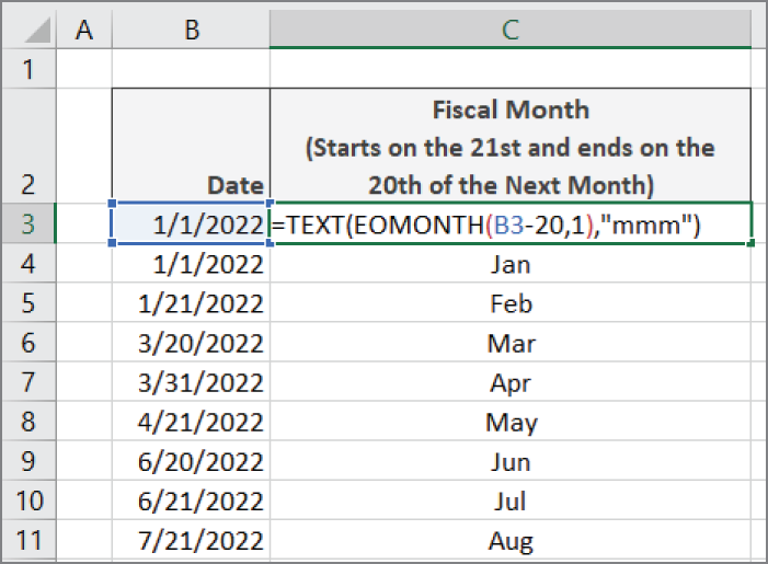
FIGURE 13.13 Calculating fiscal months
In this formula, we're first taking our date (in B3) and going back 20 days by subtracting 20. Then we are using that new date in the EOMONTH function to get the last day next month:
EOMONTH(B3-20,1)We then wrap that in a TEXT function to format the resulting date into a three-letter month name:
=TEXT(EOMONTH(B3-20,1),"mmm")Calculating the date of the Nth weekday of the month
Many analytical processes rely on knowing the dates of specific events. For example, if payroll processing occurs the second Friday of every month, it's beneficial to know which dates in the year represent the second Friday of each month.
Using the date functions covered thus far in this chapter, you can build dynamic date tables that automatically provide you with the key dates you need.
Figure 13.14 illustrates such a table. In this table, formulas calculate the Nth weekday for each month listed. The idea is to fill in the years and months you need and then tell it what number occurrence of each weekday you are seeking. In this example, cell B2 shows that we are looking for the second occurrence of each weekday.
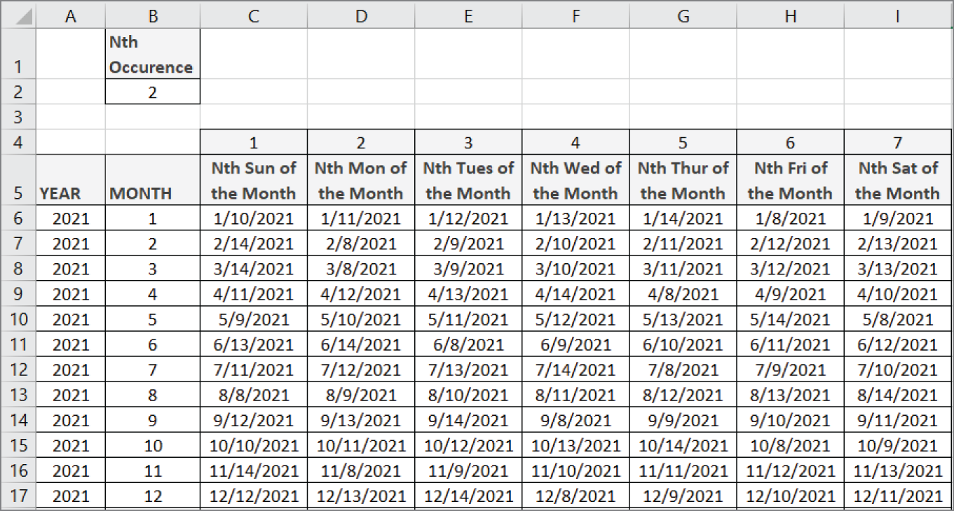
FIGURE 13.14 A dynamic date table calculating the Nth occurrence of each weekday
Cell C6 (see Figure 13.14) contains the following formula:
=DATE($A6,$B6,1)+C$4-WEEKDAY(DATE($A6,$B6,1))+($B$2-(C$4>=WEEKDAY(DATE($A6,$B6,1))))*7This formula applies some basic math to calculate which date within the month should be returned given a specific week number and occurrence.
To use the table in Figure 13.14, simply enter the years and months you are targeting, starting in cells A6 and B6. Then adjust the occurrence number you need in cell B2.
If you are looking for the first Monday of each month, enter a 1 in cell B2 and look in the Monday column. If you are looking for the third Thursday of each month, enter a 3 in cell B2 and look in the Thursday column.
Calculating the date of the last weekday of the month
You can leverage the functions covered in this chapter thus far to build a dynamic date table that automatically provides you with the last instance of a given weekday. For instance, Figure 13.15 illustrates a table that calculates the last Sunday, Monday, Tuesday, and so forth for each month listed.
Cell C4 (see Figure 13.15) contains the following formula:
=DATE($A4,$B4+1,1)-WEEKDAY(DATE($A4,$B4+1,C$2))This formula applies some basic math to calculate which date within the month should be returned given a specific year, month, and week number.
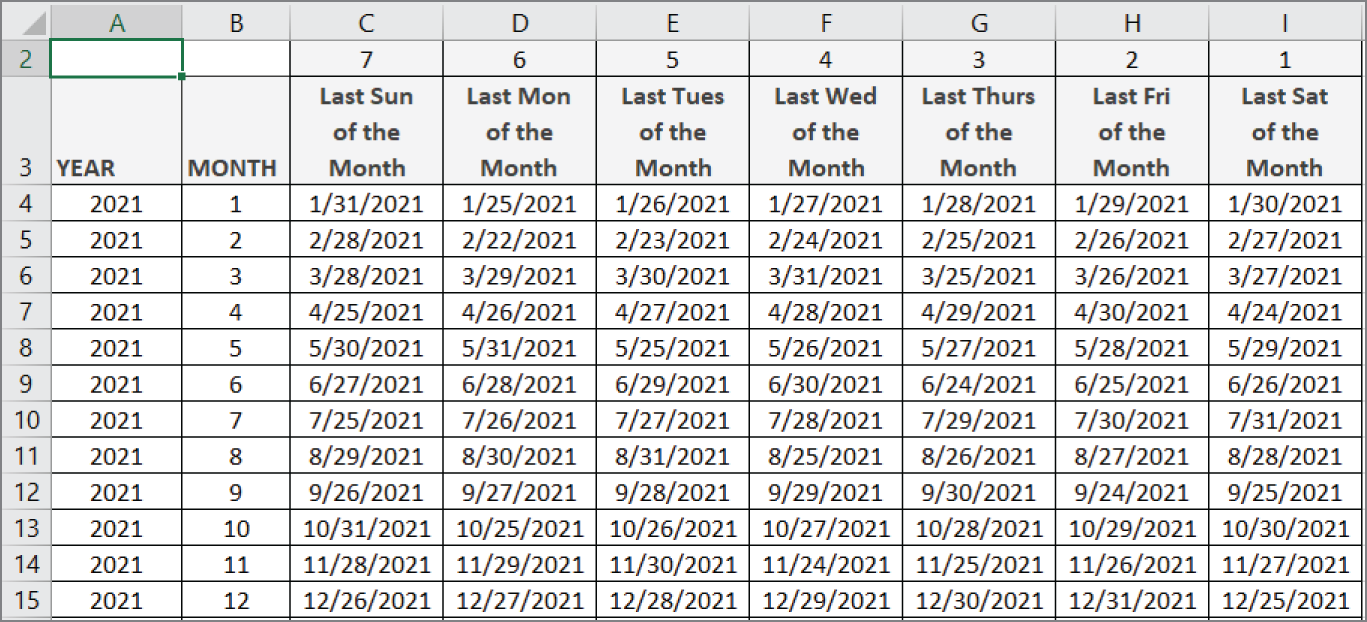
FIGURE 13.15 A dynamic date table calculating the last weekday in each month
To use the table in Figure 13.15, simply enter the years and months that you are targeting, starting in cells A4 and B4. The idea is to use this table in your Excel models as a place to which you can link or simply copy from to get the dates you need.
Extracting parts of a time
It's often helpful to pick out a specific part of a time. Excel provides a simple set of functions to parse time out into its component parts. These functions are as follows:
HOURextracts the hour portion of a given time value.MINUTEextracts the minute portion of a given time value.SECONDextracts the second portion of a given time value.
Figure 13.16 demonstrates the use of these functions to parse the time in cell C3 into its component parts.

FIGURE 13.16 Extract the parts of a time.
These functions are fairly straightforward.
The HOUR function returns a number between 0 and 23 corresponding to the hour of a given time. This formula returns 6.
=HOUR("6:15:27 AM")The MINUTE function returns a number between 0 and 59 corresponding to the minutes of a given time. This formula returns 15.
=MINUTE("6:15:27 AM")The SECOND function returns a number between 0 and 59 corresponding to the seconds of a given time. This formula returns 27.
=SECOND("6:15:27 AM")Calculating elapsed time
One of the more common calculations done with time values is calculating elapsed time, that is, how many hours and minutes between a start time and an end time.
The table in Figure 13.17 shows a list of start and end times, along with calculated elapsed times. Look at Figure 13.17, and you can see that the formula in cell D4 is as follows:
=IF(C4< B4, 1 + C4 - B4, C4 - B4) To get the elapsed time between a start and end time, all you need to do is to subtract the start time from the end time. There is a catch, however. If the end time is less than the start time, you have to assume that the clock has been running for a full 24-hour period, effectively looping back the clock.
In these cases, you have to add a 1 to the time to represent a full day. This ensures that you don't have negative elapsed times.
In our elapsed time formula, we use an IF function to check whether the end time is less than the start time. If so, we add a 1 to our simple subtraction. If not, we can just do the subtraction.
=IF(C4< B4, 1 + C4 - B4, C4 - B4)
FIGURE 13.17 Calculating elapsed time
Rounding time values
It's often necessary to round time to a particular increment. For instance, if you're a consultant, you may always want to round time up to the next 15-minute increment or down to 30-minute increments.
Figure 13.18 demonstrates how you can round to 15- and 30-minute increments.

FIGURE 13.18 Rounding time values to 15- and 30-minute increments
The formula in cell E4 is as follows:
=ROUNDUP(C4*24/0.25,0)*(0.25/24)The formula in cell F4 is as follows:
=ROUNDDOWN(C4*24/0.5,0)*(0.5/24)You can round a time value to the nearest hour by multiplying the time by 24, passing that value to the ROUNDUP function, and then dividing the result by 24. For instance, this formula would return 7:00:00 AM:
=ROUNDUP("6:15:27"*24,0)/24To round up to 15-minute increments, you simply divide 24 by 0.25 (a quarter). This formula would return 6:30:00 AM:
=ROUNDUP("6:15:27"*24/0.25,0)*(0.25/24)To round down to 30-minute increments, divide 24 by 0.5 (a half). This formula would return 6:00:00 AM:
=ROUNDDOWN("6:15:27"*24/0.5,0)*(0.5/24)
Converting decimal hours, minutes, or seconds to a time
It's not uncommon to get a feed from an external source where the times are recorded in decimal hours. For example, for 1 hour and 30 minutes, you see 1.5 instead of the standard 1:30. You can easily correct this by dividing the decimal hour by 24 and then formatting the result as a time.
Figure 13.19 shows some example decimal hours and the converted times.
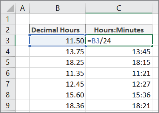
FIGURE 13.19 Converting decimal hours to hours and minutes
Dividing the decimal hour by 24 will result in a decimal that Excel recognizes as a time value.
To convert decimal minutes into time, divide the number by 1440. This formula will return 1:04 (one hour and four minutes):
=64.51/1440To convert decimal seconds into time, divide the number by 86400. This formula will return 0:06 (six minutes):
=390.45/86400Adding hours, minutes, or seconds to a time
Because time values are nothing more than a decimal extension of the date serial number system, you can add two time values together to get a cumulative time value. In some cases, you may want to add a set number of hours and minutes to an existing time value. In these situations, you can use the TIME function.
Cell D4 in Figure 13.20 contains this formula:
=C4+TIME(5,30,0) In this example, we're adding 5 hours and 30 minutes to all of the times in the list.

FIGURE 13.20 Adding a set number of hours and minutes to an existing time value
The TIME function lets you build a time value on the fly using three arguments: hour, minute, and second. For example, this formula would return the time value 2:30:30 PM:
=TIME(14,30,30)To add a certain number of hours to an existing time value, simply use the TIME function to build a new time value and then add them together. This formula adds 30 minutes to the existing time, resulting in a time value of 3:00:00 PM:
="2:30:00 PM"+TIME(0,30,0)