CHAPTER 11
Using Formulas for Common Mathematical Operations
Most Excel analysts working in the corporate world will be asked to perform mathematical operations that provide insight into key operational metrics. In this chapter, you'll get to explore a few mathematical operations commonly used in the world of business analytics.
Calculating Percentages
Calculations such as percent of totals, variance to budget, and running totals are the cornerstone of any basic business analysis. In the following sections, you'll explore some examples of formulas that will help with these types of analyses.
Calculating percent of goal
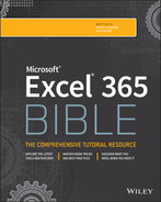
When someone asks you to calculate a percent of goal, they are simply asking you to compare the actual performance against a stated goal. The math involved in this calculation is simple: divide the actual by the goal. This will give you a percentage value that represents how much of the goal has been achieved. For instance, if your goal is to sell 100 widgets and you sell 80 widgets, your percent of goal is 80% (80/100).
Figure 11.1 shows a list of regions with a column for goals and a column for actuals. Note that the formula in cell E5 simply divides the value in the Actual column by the value in the Goal column.
=D5/C5 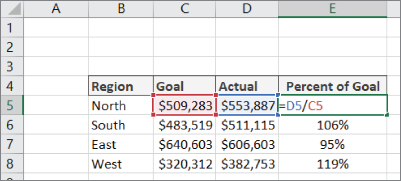
FIGURE 11.1 Calculating the percent of goal
There isn't much to this formula. You're simply using cell references to divide one value by another. You can enter the formula one time in the first row (cell E5 in this case) and then copy that formula down to every other row in your table.
Alternatively, if you need to compare actuals to a common goal, you can set up a model like the one shown in Figure 11.2. In this model, each region does not have its own goal. Instead, you're comparing the values in the Actual column to a single goal found in cell B3.
=C6/$B$3 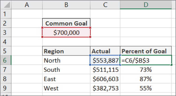
FIGURE 11.2 Calculating the percent of goal using a common goal
Note that the cell reference to the common goal is entered as an absolute reference ($B$3). Using the dollar symbols locks the reference to the goal in place, ensuring that the cell reference pointing to the common goal does not adjust as you copy the formula down.
Calculating percent variance
A variance is an indicator of the difference between one number and another. To understand this, imagine that you sold 120 widgets one day, and on the next day, you sold 150 widgets. The difference in sales in actual terms is easy to see; you sold 30 more widgets on the second day, and 150 widgets minus 120 widgets gives you a unit variance of +30.
So, what is a percent variance? This is essentially the percentage difference between the benchmark number (120) and the new number (150). You calculate the percent variance by subtracting the benchmark number from the new number and then dividing that result by the benchmark number; In this example, (150-120)/120 = 25%. The percent variance tells us that you sold 25% more widgets than on the previous day.
Figure 11.3 demonstrates how to translate this into a formula. The formula in E4 calculates the percent variance between current year sales and previous year sales.
=(D4-C4)/C4 
FIGURE 11.3 Calculating the percent variance between current year sales and previous year sales
The one thing to note about this formula is the use of parentheses. By default, Excel's order of operations states that division must be done before subtraction. But if we let that happen, we would get an erroneous result. Wrapping the first part of the formula in parentheses ensures that Excel performs subtraction before the division.
You can simply enter the formula one time in the first row (cell E4 in this case) and then copy that formula down to every other row in your table.
An alternative formula for calculating percent variance is simply to divide the current year's sales by the previous year's sales and then subtract 1. Because Excel performs division operations before subtraction, you don't have to use parentheses with this alternative formula.
=D4/C4-1Calculating percent variance with negative values
In the previous section, “Calculating percent variance,” you discovered how to calculate a percent variance. This works beautifully in most cases. However, when the benchmark value is a zero or less, the formula breaks down.
For example, imagine you're starting a business and expect to take a loss during the first year. So, you give yourself a budget of negative $10,000. Now imagine that after your first year, you made money, earning $12,000. Calculating the percent variance between your actual revenue and budgeted revenue would give you –220%. You can try it on a calculator. 12,000 minus –10,000 divided by –10,000 equals –220%.
How can you say that your percent variance is –220% when you clearly made money? Well, the problem is that when your benchmark value is a negative number, the math inverts the results, causing numbers to look wacky. This is a real problem in the corporate world, where budgets can often be negative values.
The fix is to leverage the ABS function to negate the negative benchmark value:
=(C4-B4)/ABS(B4)Figure 11.4 uses this formula in cell E4, illustrating the different results you get when using the standard percent variance formula and the improved percent variance formula.

FIGURE 11.4 Using the ABS function will give you an accurate percent variance when dealing with negative values.
Excel's ABS function returns the absolute value for any number you pass to it. Entering =ABS(-100) into cell A1 would return 100. The ABS function essentially makes any number a non-negative number. Using ABS in this formula negates the effect of the negative benchmark (the negative 10,000 budget in our example) and returns the correct percent variance.
Calculating a percent distribution
Percent distribution is a measure of how a metric (such as total revenue) is distributed among the components that make up the total. As you can see in Figure 11.5, the calculation is relatively simple. You divide each component by the total. In this example, we have a cell that contains the total revenue (cell C9). We then divide each region's revenue by the total to get a percent distribution for each region.
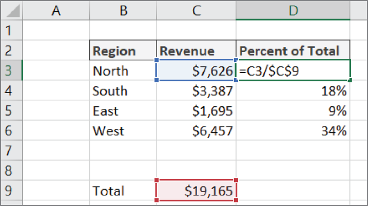
FIGURE 11.5 Calculating a percent distribution of revenue across regions
There isn't much to this formula. You're simply using cell references to divide each component value by the total. The one thing to note is that the cell reference to the total is entered as an absolute reference ($C$9). Using the dollar symbols locks the reference in place, ensuring that the cell reference pointing to the total value does not adjust as you copy the formula down.
You don't have to dedicate a separate cell to an actual total value. You can simply calculate the total on the fly within the percent distribution formula. Figure 11.6 demonstrates how you can use the SUM function in place of a cell dedicated to holding a total value. The SUM function adds together any numbers you pass to it.

FIGURE 11.6 Calculating percent distribution with the SUM function
Again, note the use of absolute references in the SUM function. This ensures that the SUM range stays locked as you copy the formula down.
=C3/SUM($C$3:$C$6)Calculating a running total
Some organizations like to see a running total as a mechanism to analyze the changes in a metric as a period of time progresses. Figure 11.7 illustrates a running total of units sold for January through December. The formula used in cell D3 is copied down to each month.
=SUM($C$3:C3) 
FIGURE 11.7 Calculating a running total
In this formula, the SUM function is used to add up all the units from cell C3 to the current row. The trick to this formula is the absolute reference ($C$3). Placing an absolute reference in the reference for the first value of the year locks that value down. This ensures that as the formula is copied down, the SUM function will always capture and add the units from the first value to the value on the current row.
Applying a percent increase or decrease to values
A common task for an Excel analyst is to apply a percentage increase or decrease to a given number. For instance, when applying a price increase to a product, you would typically raise the original price by a certain percent. When giving a customer a discount, you would decrease that customer's rate by a certain percent.
Figure 11.8 illustrates how to apply a percent increase and decrease using a simple formula. In cell E5, we're applying a 10% price increase to Product A. In cell E9, we're giving a 20% discount to Customer A.
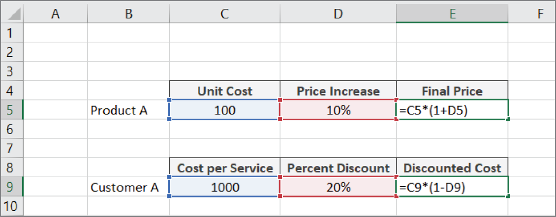
FIGURE 11.8 Applying a percent increase and decrease using a simple formula
To increase a number by a percentage amount, multiply the original amount by 1 plus the percent of increase. In the example in Figure 11.8, Product A is getting a 10% increase. So, we first add 1 to the 10%. This gives us 110%. We then multiply the original price of 100 by 110%. This calculates to the new price of 110.
To decrease a number by a percentage amount, multiply the original amount by 1, which is the percent discount. In the example in Figure 11.8, Customer A is getting a 20% discount. So, we first subtract 20% from 1. This gives us 80%. We then multiply the original 1000 cost per service by 80%. This calculates to the new rate of 800.
Note the use of parentheses in the formulas. By default, Excel's order of operations states that multiplication must be done before addition or subtraction. But if we let that happen, we would get an erroneous result. Wrapping the second part of the formula in parentheses ensures that Excel performs the multiplication last.
Dealing with divide-by-zero errors
In mathematics, division by zero is impossible. One way to understand why it's impossible is to consider what happens when you divide a number by another.
Division is really nothing more than fancy subtraction. For example, 10 divided by 2 is the same as starting with 10 and continuously subtracting 2 as many times as needed to get to zero. In this case, you would need to continuously subtract 2 five times.
- 10 − 2 = 8
- 8 − 2 = 6
- 6 − 2 = 4
- 4 − 2 = 2
- 2 − 2 = 0
So, 10/2 = 5.
Now if you tried to do this with 10 divided by 0, you would never get anywhere because 10 − 0 is 10 all day long. You'd be sitting there subtracting 0 until your calculator dies.
- 10 − 0 = 10
- 10 − 0 = 10
- 10 − 0 = 10
- 10 − 0 = 10
- …infinity
Mathematicians call the result you get when dividing any number by zero undefined. Software like Excel simply gives you an error when you try to divide by zero. In Excel, when you divide a number by zero, you get the #DIV/0! error.
You can avoid this by telling Excel to skip the calculation if your denominator is a zero. Figure 11.9 illustrates how to do this by wrapping the division operation in Excel's IF function.
=IF(C4=0,0,D4/C4) 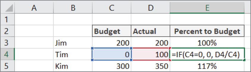
FIGURE 11.9 Using the IF function to avoid a division-by-zero error
The IF function has three arguments: the condition, what to do if the condition is true, and what to do if the condition is false.
The condition argument in this example is that the budget in C4 is equal to zero (C4=0). Condition arguments must be structured to return TRUE or FALSE, which usually means there is a comparison operation (such as an equal sign or greater-than sign) or another worksheet function that returns TRUE or FALSE (like ISERR or ISBLANK).
If our condition argument returns TRUE, the second argument of the IF function is returned to the cell. Our second argument is 0, meaning that we simply want a zero displayed if the budget number in cell C4 is a zero.
If the condition argument is not zero, the third argument takes effect. In our third argument, we tell Excel to perform the division calculation (D4/C4).
So, this formula states that if C4 equals 0, then return a 0; otherwise, return the result of D4/C4.
Rounding Numbers
Often, your customers will want to look at clean, round numbers. Inundating a user with decimal values and unnecessary digits for the sake of precision can make your reports harder to read. For this reason, you may consider using Excel's rounding functions.
In the following sections, you'll explore some of the techniques that you can leverage to apply rounding to your calculations.
Rounding numbers using formulas
Excel's ROUND function is used to round a given number to a specified number of digits. The ROUND function takes two arguments: the original value and the number of digits to round to.
Passing 0 as the second argument tells Excel to remove all decimal places and round the integer portion of the number based on the first decimal place. For instance, this formula rounds to 94:
=ROUND(94.45,0)Passing a 1 as the second argument tells Excel to round to one decimal based on the value of the second decimal place. For example, this formula rounds to 94.5:
=ROUND(94.45,1)You can also pass a negative number to the second argument, telling Excel to round based on values to the left of the decimal point. The following formula, for example, returns 90:
=ROUND(94.45,-1)You can force rounding in a particular direction using the ROUNDUP or ROUNDDOWN function.
This ROUNDDOWN formula rounds 94.45 down to 94:
=ROUNDDOWN(94.45,0)This ROUNDUP formula rounds 94.45 up to 95:
=ROUNDUP(94.45,0)Rounding to the nearest penny
In some industries, it is common practice to round a dollar amount to the nearest penny. Figure 11.10 demonstrates how rounding a dollar amount up or down to the nearest penny can affect the resulting number.
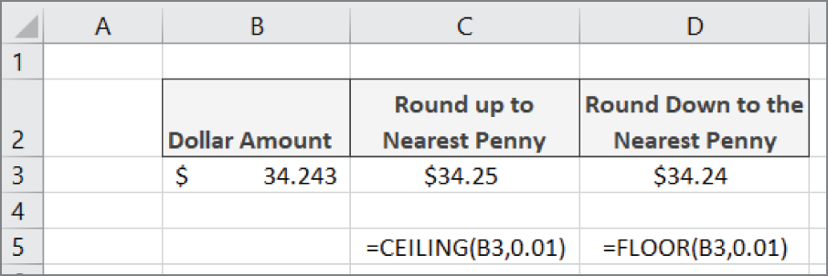
FIGURE 11.10 Rounding to the nearest penny
You can round to the nearest penny by using the CEILING or FLOOR function.
The CEILING function will round a number up to the nearest multiple of significance that you pass to it. This comes in handy when you need to override the standard rounding protocol with your own business rules. For instance, you can force Excel to round 123.222 to 124 by using the CEILING function with a significance of 1:
=CEILING(123.222,1)So, passing a .01 as the significance tells the CEILING function to round up to the nearest penny.
If you wanted to round up to the nearest nickel, you can use .05 as the significance. For instance, the following formula returns 123.15:
=CEILING(123.11,.05)The FLOOR function works the same way except it forces a rounding down to the nearest significance. The following example function rounds 123.19 down to the nearest nickel, giving you 123.15 as the result:
=FLOOR(123.19,.05)Rounding to significant digits
In some financial reports, figures are presented in significant digits. The idea is that when you're dealing with numbers in the millions, there is no need to inundate a report with superfluous numbers for the sake of showing precision down to the tens, hundreds, and thousands place.
For instance, instead of showing the number 883,788, you could choose to round the number to one significant digit. This would mean displaying the same number as 900,000. Rounding 883,788 to two significant digits would show the number as 880,000.
In essence, you're deeming that a particular number's place is significant enough to show. The rest of the number can be replaced with zeros. This may feel like it could introduce problems, but when dealing with large enough numbers, any number below a certain significance would be inconsequential.
Figure 11.11 demonstrates how you can implement a formula that rounds numbers to a given number of significant digits.
Let's take a moment to see how this works.
Excel's ROUND function is used to round a given number to a specified number of digits. The ROUND function takes two arguments: the original value and number of digits to round to.
Passing a negative number to the second argument tells Excel to round based on significant digits to the left of the decimal point. The following formula, for example, returns 9500:
=ROUND(9489,-2)
FIGURE 11.11 Rounding numbers to one significant digit
Changing the significant digits argument to –3 will return a value of 9000.
=ROUND(9489,-3)This works great, except what if we have numbers on differing scales? In other words, what if some of our numbers are millions while others are hundreds of thousands? If we wanted to display all our numbers in one significant digit, we would need to build a different ROUND function for each number to account for the differing significant digits argument that we would need for each type of number.
To help solve this, we can replace our hard-coded significant digits argument with a formula that calculates what that number should be.
Imagine that our number is –2330.45. We can use this formula as the significant digits argument in our ROUND function:
LEN(INT(ABS(-2330.45)))*-1+2This formula first wraps our number within the ABS function, effectively removing any negative symbol that may exist. It then wraps that result in the INT function, stripping out any decimals that may exist. Finally, it wraps that result in the LEN function to get a measure of how many digits are in the number without any decimals or negation symbols.
In the example, this part of the formula results in 4. If you take the number –2330.45 and strip away the decimals and negative symbol, you have four digits left.
This number is then multiplied by –1 to make it a negative number, and it is then added to the number of significant digits we are seeking. In this example, 4*-1+2 = –2.
Again, this formula will be used as the second argument for our ROUND function. Enter this formula into Excel, and you'll round this number to –2300 (two significant digits).
=ROUND(-2330.45,LEN(INT(ABS(-2330.45)))*-1+2)You can then replace this formula with cell references that point to the source number and cell that holds the number of desired significant digits. This is what you saw in Figure 11.11.
=ROUND(B5,LEN(INT(ABS(B5)))*-1+$E$3)Counting Values in a Range
Excel provides several functions to count the values in a range: COUNT, COUNTA, and COUNTBLANK. Each of these functions provides a different method of counting based on whether the values are numbers, numbers and text, or blank.
Figure 11.12 illustrates the different kinds of counting that you can perform. In row 12, we are using the COUNT function to count only the exams where students have passed. In column H, we are using the COUNTA function to count all the exams taken by a student. In column I, we are using the COUNTBLANK function to count only those exams that have not yet been taken.
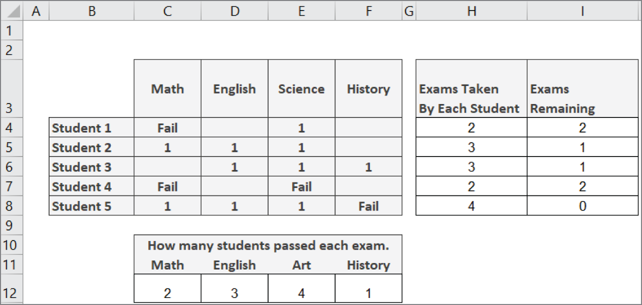
FIGURE 11.12 A demonstration of counting cells
The COUNT function will count only numeric values in a given range. It requires only a single argument where you pass a range of cells. For example, this formula will count only those cells in range C4:C8 that contain a numeric value:
=COUNT(C4:C8)The COUNTA function will count any cell that is not blank. This function can be used when counting cells that contain any combination of numbers and text. It requires only a single argument where you pass a range of cells. For instance, this formula will count all the nonblank cells in range C4:F4
:
=COUNTA(C4:F4)The COUNTBLANK function will count only the blank cells in a given range. It requires only a single argument where you pass a range of cells. For instance, this formula will count all the blank cells in range C4:F4
:
=COUNTBLANK(C4:F4)Using Excel's Conversion Functions
You may work at a company where it's important to know how many cubic yards can be covered by a gallon of material or how many cups are needed to fill an Imperial gallon.
You can use Excel's CONVERT function to produce a conversion table containing every possible type of conversion you need for a set of measures. Figure 11.13 illustrates a conversion table created using nothing but Excel's CONVERT function.
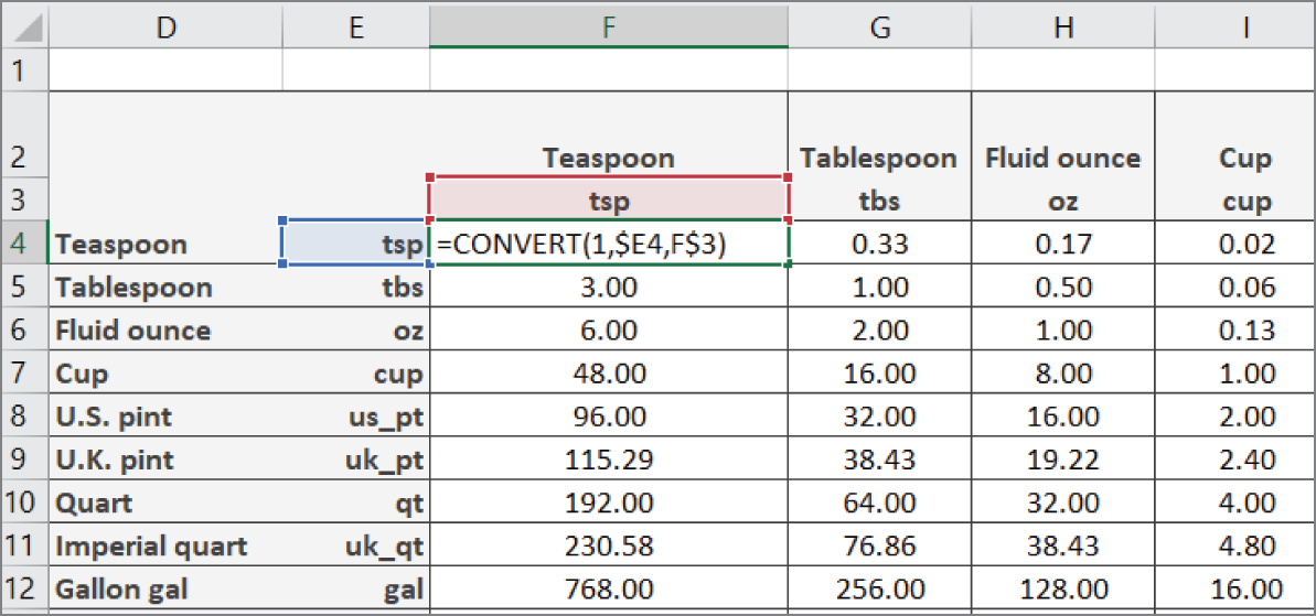
FIGURE 11.13 Creating a unit-of-measure conversion table
With this table, you can get a quick view of the conversions from one unit of measure to another. You can see that it takes 48 teaspoons to make a cup, 2.4 cups to make an English pint, and so forth.
The CONVERT function requires three arguments: a number value, the unit you're converting from, and the unit you're converting to. For instance, to convert 100 miles into kilometers, you can enter this formula to get the answer 160.93:
=CONVERT(100,"mi","km")You can use the following formula to convert 100 gallons into liters. This will give you the result of 378.54:
=CONVERT(100,"gal","l")You'll notice the conversion codes for each unit of measure. These codes are specific and must be entered exactly how Excel expects to see them. Entering a CONVERT formula using gallon or GAL instead of the expected gal will return an error.
Luckily, Excel provides a ScreenTip as you start entering your CONVERT function, letting you pick the correct unit codes from a list.
You can refer to Excel's help files on the CONVERT function to get a list of valid units of measure conversion codes.
Once you have the codes in which you are interested, you can enter them in a matrix-style table like the one you saw in Figure 11.13. In the top-left cell in your matrix, enter a formula that points to the appropriate conversion code for the matrix row and matrix column.
Be sure to include the absolute references necessary to lock the references to the conversion codes. For the codes located in the matrix row, lock to the column reference. For the codes located in the matrix column, lock the row reference.
=CONVERT(1,$E4,F$3)At this point, you can simply copy your formula across the entire matrix.