
Thus far the reliability and quality management models we have discussed are either at the project or the product level. Both types of model tend to treat the software more or less as a black box. In other words, they are based on either the external behavior (e.g., failure data) of the product or the intermediate process data (e.g., type and magnitude of inspection defects), without looking into the internal dynamics of design and code of the software. In this chapter we describe the relationships between metrics about design and code implementation and software quality. The unit of analysis is more granular, usually at the program-module level. Such metrics and models tend to take an internal view and can provide clues for software engineers to improve the quality of their work.
Reliability models are developed and studied by researchers and software reliability practitioners with sophisticated skills in mathematics and statistics; quality management models are developed by software quality professionals and product managers for practical project and quality management. Software complexity research, on the other hand, is usually conducted by computer scientists or experienced software engineers. Like the reliability models, many complexity metrics and models have emerged in the recent past. In this chapter we discuss several key metrics and models, and describe a real-life example of metric analysis and quality improvement.
The lines of code (LOC) count is usually for executable statements. It is actually a count of instruction statements. The interchangeable use of the two terms apparently originated from Assembler program in which a line of code and an instruction statement are the same thing. Because the LOC count represents the program size and complexity, it is not a surprise that the more lines of code there are in a program, the more defects are expected. More intriguingly, researchers found that defect density (defects per KLOC) is also significantly related to LOC count. Early studies pointed to a negative relationship: the larger the module size, the smaller the defect rate. For instance, Basili and Perricone (1984) examined FORTRAN modules with fewer than 200 lines of code for the most part and found higher defect density in the smaller modules. Shen and colleagues (1985) studied software written in Pascal, PL/S, and Assembly language and found an inverse relationship existed up to about 500 lines. Since larger modules are generally more complex, a lower defect rate is somewhat counterintuitive. Interpretation of this finding rests on the explanation of interface errors: Interface errors are more or less constant regardless of module size, and smaller modules are subject to higher error density because of smaller denominators.
More recent studies point to a curvilinear relationship between lines of code and defect rate: Defect density decreases with size and then curves up again at the tail when the modules become very large. For instance, Withrow (1990) studied modules written in Ada for a large project at Unisys and confirmed the concave relationship between defect density (during formal test and integration phases) and module size (Table 11.1). Specifically, of 362 modules with a wide range in size (from fewer than 63 lines to more than 1,000), Withrow found the lowest defect density in the category of about 250 lines. Explanation of the rising tail is readily available. When module size becomes very large, the complexity increases to a level beyond a programmer’s immediate span of control and total comprehension. This new finding is also consistent with previous studies that did not address the defect density of very large modules.
Experience from the AS/400 development also lends support to the curvilinear model. In the example in Figure 11.1, although the concave pattern is not as significant as that in Withrow’s study, the rising tail is still evident.

The curvilinear model between size and defect density sheds new light on software quality engineering. It implies that there may be an optimal program size that can lead to the lowest defect rate. Such an optimum may depend on language, project, product, and environment; apparently many more empirical investigations are needed. Nonetheless, when an empirical optimum is derived by reasonable methods (e.g., based on the previous release of the same product, or based on a similar product by the same development group), it can be used as a guideline for new module development.
Halstead (1977) distinguishes software science from computer science. The premise of software science is that any programming task consists of selecting and arranging a finite number of program “tokens,” which are basic syntactic units distinguishable by a compiler. A computer program, according to software science, is a collection of tokens that can be classified as either operators or operands. The primitive measures of Halstead’s software science are:
Based on these primitive measures, Halstead developed a system of equations expressing the total vocabulary, the overall program length, the potential minimum volume for an algorithm, the actual volume (number of bits required to specify a program), the program level (a measure of software complexity), program difficulty, and other features such as development effort and the projected number of faults in the software. Halstead’s major equations include the following:
|
Vocabulary (n) |
|
|
Length (N) |
|
|
Volume (V) |
|
|
Level (L) |
|
|
Difficulty (D) (inverse of level) |
|
|
Effort (E) |
|
|
Faults (B) |
|
where V* is the minimum volume represented by a built-in function performing the task of the entire program, and S* is the mean number of mental discriminations (decisions) between errors (S* is 3,000 according to Halstead).
Halstead’s work has had a great impact on software measurement. His work was instrumental in making metrics studies an issue among computer scientists. However, software science has been controversial since its introduction and has been criticized from many fronts. Areas under criticism include methodology, derivations of equations, human memory models, and others. Empirical studies provide little support to the equations except for the estimation of program length. Even for the estimation of program length, the usefulness of the equation may be subject to dispute. To predict program length, data on N1 and N2 must be available, and by the time N1 and N2 can be determined, the program should be completed or near completion. Therefore, the predictiveness of the equation is limited. As discussed in Chapter 3, both the formula and actual LOC count are functions of N1 and N2; thus they appear to be just two operational definitions of the concept of program length. Therefore, correlation exists between them by definition.
In terms of quality, the equation for B appears to be oversimplified for project management, lacks empirical support, and provides no help to software engineers. As S* is taken as a constant, the equation for faults (B) simply states that the number of faults in a program is a function of its volume. This metric is therefore a static metric, ignoring the huge variations in fault rates observed in software products and among modules.
The measurement of cyclomatic complexity by McCabe (1976) was designed to indicate a program’s testability and understandability (maintainability). It is the classical graph theory cyclomatic number, indicating the number of regions in a graph. As applied to software, it is the number of linearly independent paths that comprise the program. As such it can be used to indicate the effort required to test a program. To determine the paths, the program procedure is represented as a strongly connected graph with unique entry and exit points. The general formula to compute cyclomatic complexity is:
where
|
V(G) |
= Cyclomatic number of G |
|
e |
= Number of edges |
|
n |
= Number of nodes |
|
p |
= Number of unconnected parts of the graph |
As an example, Figure 11.2 is a control graph of a simple program that might contain two IF statements. If we count the edges, nodes, and disconnected parts of the graph, we see that e = 8, n = 7, and p = 1, and that M = 8 – 7 + 2 * 1 = 3.
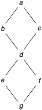
Note that M is also equal to the number of binary decisions in a program plus 1. If all decisions are not binary, a three-way decision is counted as two binary decisions and an n-way case (select) statement is counted as n – 1 binary decisions. The iteration test in a looping statement is counted as one binary decision. In the preceding simple example, since there are two binary decisions, M = 2 + 1 = 3.
The cyclomatic complexity metric is additive. The complexity of several graphs considered as a group is equal to the sum of the individual graphs’ complexities. However, it ignores the complexity of sequential statements. Neither does the metric distinguish different kinds of control flow complexity such as loops versus IF-THEN-ELSE statements or cases versus nested IF-THEN-ELSE statements.
To have good testability and maintainability, McCabe recommends that no program module should exceed a cyclomatic complexity of 10. Because the complexity metric is based on decisions and branches, which is consistent with the logic pattern of design and programming, it appeals to software professionals. Since its inception, cyclomatic complexity has become an active area of research and practical applications. Many experts in software testing recommend use of the cyclomatic representation to ensure adequate test coverage; the use of McCabe’s complexity measure has been gaining acceptance by practitioners.
Because of its appeal to programmers and researchers, many studies have been conducted to relate McCabe’s complexity measure to defect rate, and moderate to strong correlations were observed. For instance, in a study of software metrics of a large SQL product that consisted of about 1300 modules, Troster (1992) found a relatively strong correlation between McCabe’s cyclomatic complexity index and the number of test defects (r = .48, n = 1303, p = .0001). Studies found that the complexity index also correlates strongly with program size—lines of code. Will the correlation between complexity and defect remain significant after program size is controlled? In other words, is the correlation between complexity and defects a spurious one, because program size affects both complexity and defect level? Many studies have been done with regard to this question and the findings are not always consistent. There are cases where the correlation disappears after the effect of program size is controlled; in other cases the correlation weakens somewhat but remains significant, suggesting a genuine association between complexity and defect level. Our experience belongs to the latter kind.
Sometimes the disappearance of the correlation between complexity and defect level after accounting for program size may be due to a lack of investigational rigor. It is important that appropriate statistical techniques be used with regard to the nature of the data. For example, Troster observed that the LOC count also correlated with the number of test defects quite strongly (r = 0.49, n = 1296, p = 0.001). To partial out the effect of program size, therefore, he calculated the correlation between McCabe’s complexity index and testing defect rate (per KLOC). He found that the correlation totally disappeared with r = 0.002 (n = 1296, p = 0.9415). Had Troster stopped there, he would have concluded that there is no genuine association between complexity and defect level. Troster realized, however, that he also needed to look at the rank-order correlation. Therefore, he also computed the Spearman’s rank-order correlation coefficient and found a very respectable association between complexity and defect rate:
Spearman’s correlation = 0.27
n = 1296 (number of modules)
p = 0.0001 (highly statistically significant)
These seemingly inconsistent findings, based on our experience and observation of the Troster study, is due to the nature of software data. As discussed previously, Pearson’s correlation coefficient is very sensitive to extreme data points; it can also be distorted if there is a lot of noise in the data. Defect rate data (normalized to KLOC) tend to fluctuate widely and therefore it is difficult to have significant Pearson correlation coefficients. The rank-order correlation coefficient, which is less precise but more robust than the Pearson correlation coefficient, is more appropriate for such data.
As another example, Craddock (1987) reports the use of McCabe’s complexity index at low-level design inspections and code inspection (I2). He correlated the number of inspection defects with both complexity and LOC. As shown in Table 11.2, Craddock found that complexity is a better indicator of defects than LOC at the two inspection phases.
Assuming that an organization can establish a significant correlation between complexity and defect level, then the McCabe index can be useful in several ways, including the following:
Table 11.2. Correlation Coefficients Between Inspection Defects and Complexity
|
Inspection Type |
Number of Inspections |
KLOC |
r Lines of Code |
r McCabe’s Index |
|---|---|---|---|---|
|
I0 |
46 |
129.9 |
0.10 |
— |
|
I1 |
41 |
67.9 |
0.46 |
0.69 |
|
I2 |
30 |
35.3 |
0.56 |
0.68 |
To help identify overly complex parts needing detailed inspections
To help identify noncomplex parts likely to have a low defect rate and therefore candidates for development without detailed inspections
To estimate programming and service effort, identify troublesome code, and estimate testing effort
Later in this chapter we describe an example of complexity study in more detail and illustrate how quality improvement can be made via the focus on complexity reduction.
McCabe’s cyclomatic complexity index is a summary index of binary decisions. It does not distinguish different kinds of control flow complexity such as loops versus IF-THEN-ELSES or cases versus IF-THEN-ELSES. Researchers of software metrics also studied the association of individual syntactic constructs with defect level. For instance, Shen and associates (1985) discovered that the number of unique operands (n2) was useful in identifying the modules most likely to contain errors for the three software products they studied. Binder and Poore (1990) empirically supported the concept of local software quality metrics whose formulation is based on software syntactic attributes. Such local metrics may be specific to the products under study or the development teams or environments. However, as long as an empirical association with software quality is established, those metrics could provide useful clues for improvement actions. In selecting such metrics for study, consideration must be given to the question of whether the metric could be acted on.
In studying the quality and syntactic indicators among a sample of twenty modules of a COBOL compiler product, Lo (1992) found that field defects at the module level can be estimated through the following equations:
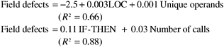
While both equations provide satisfactory results, the findings mean nothing in terms of planning actions for improvement. In a second attempt, which included all 66 modules of the product, Lo examined other syntactic constructs and found the following relationship:
In the model, all three metrics are statistically significant, with DO WHILE having the most effect. The DO WHILE metric included both DO WHILE . . . END and DO WHILE TO . . . . ? Although the R2 of the model decreased, the findings provide useful clues for improvement. Although it is difficult to avoid the use of IF THEN or to change the number of unique operands, it is feasible to reduce the use of a complex construct such as the DO WHILE or SELECT statement. Upon brainstorming with the development team, Lo found that most developers were having difficulty mastering the DO WHILE construct. As a result, minimizing the use of DO WHILE was one of the actions the team took to reduce defects in the compiler product.
Lines of code, Halstead’s software science, McCabe’s cyclomatic complexity, and other metrics that measure module complexity assume that each program module is a separate entity. Structure metrics try to take into account the interactions between modules in a product or system and quantify such interactions. Many approaches in structure metrics have been proposed. Some good examples include invocation complexity by McClure (1978), system partitioning measures by Belady and Evangelisti (1981), information flow metrics by Henry and Kafura (1981), and stability measures by Yau and Collofello (1980). Many of these metrics and models, however, are yet to be verified by empirical data from software development projects.
Perhaps the most common design structure metrics are the fan-in and fan-out metrics, which are based on the ideas of coupling proposed by Yourdon and Constantine (1979) and Myers (1978):
Fan-in: A count of the modules that call a given module
Fan-out: A count of modules that are called by a given module
In general, modules with a large fan-in are relatively small and simple, and are usually located at the lower layers of the design structure. In contrast, modules that are large and complex are likely to have a small fan-in. Therefore, modules or components that have a large fan-in and large fan-out may indicate a poor design. Such modules have probably not been decomposed correctly and are candidates for re-design. From the complexity and defect point of view, modules with a large fan-in are expected to have negative or insignificant correlation with defect levels, and modules with a large fan-out are expected to have a positive correlation. In the AS/400 experience, we found a positive correlation between fan-out and defect level, and no correlation between fan-in and defects. However, the standard deviations of fan-in and fan-out were quite large in our data. Therefore, our experience was inconclusive.
Henry and Kafura’s structure complexity is defined as:
In an attempt to incorporate the module complexity and structure complexity, Henry and Selig’s work (1990) defines a hybrid form of their information-flow metric as
where Cip is the internal complexity of procedure p, which can be measured by any module complexity metrics such as McCabe’s cyclomatic complexity.
Based on various approaches to structure complexity and module complexity measures, Card and Glass (1990) developed a system complexity model
where
Ct = System complexity
St = Structural (intermodule) complexity
Dt = Data (intramodule) complexity
They defined relative system complexity as
where n is the number of modules in the system.
Structure complexity is further defined as
where
S = Structural complexity
f (i)= Fan-out of module i
n = Number of modules in system
and data complexity is further defined as
where
Di = Data complexity of module i
V(i)= I/O variables in module i
f (i)= Fan-out of module i.
where
D = Data (intramodule) complexity
D(i)= Data complexity of module i
n = Number of new modules in system
Simply put, according to Card and Glass (1990), system complexity is a sum of structural (intermodule) complexity and overall data (intramodule) complexity. Structural complexity is defined as the mean (per module) of squared values of fan-out. This definition is based on the findings in the literature that fan-in is not an important complexity indicator and that complexity increases as the square of connections between programs (fan-out). With regard to data (intramodule) complexity of a module, it is defined as a function that is directly dependent on the number of I/O variables and inversely dependent on the number of fan-outs in the module. The rationale is that the more I/O variables in a module, the more functionality needs to be accomplished by the module and, therefore, the higher internal complexity. On the contrary, more fan-out means that functionality is deferred to modules at lower levels, therefore, the internal complexity of a module is reduced. Finally, the overall data complexity is defined as the average of data complexity of all new modules. In Card and Glass’s model, only new modules enter the formula because oftentimes the entire system consists of reused modules, which have been designed, used, aged, and stabilized in terms of reliability and quality.
In a study of eight software projects, Card and Glass found that the system complexity measure was significantly correlated with subjective quality assessment by a senior development manager and with development error rate. Specifically, the correlation between system complexity and development defect rate was 0.83, with complexity accounting for fully 69% of the variation in error rate. The regression formula thus derived was
In other words, each unit increase in system complexity increases the error rate by 0.4 (errors per thousand lines of code).
The Card and Glass model appears quite promising and has an appeal to software development practitioners. They also provide guidelines on achieving a low complexity design. When more validation studies become available, the Card and Glass model and related methods may gain greater acceptance in the software development industry.
While Card and Glass’s model is for the system level, the system values of the metrics in the model are aggregates (averages) of module-level data. Therefore, it is feasible to correlate these metrics to defect level at the module level. The meanings of the metrics at the module level are as follows:
Di = data complexity of module i, as defined earlier
Si = structural complexity of module i, that is, a measure of the module’s interaction with other modules
Ci = Si + Di = the module’s contribution to overall system complexity
In Troster’s study (1992) discussed earlier, data at the module level for Card and Glass’s metrics are also available. It would be interesting to compare these metrics with McCabe’s cyclomatic complexity with regard to their correlation with defect rate. Not unexpectedly, the rank-order correlation coefficients for these metrics are very similar to that for McCabe’s (0.27). Specifically, the coefficients are 0.28 for Di, 0.19 for Si, and 0.27 for Ci. More research in this area will certainly yield more insights into the relationships of various design and module metrics and their predictive power in terms of software quality.
In this section, we describe an analysis of several module design metrics as they relate to defect level, and how such metrics can be used to develop a software quality improvement plan. Special attention is given to the significance of cyclomatic complexity. Data from all program modules of a key component in the AS/400 software system served as the basis of the analysis. The component provides facilities for message control among users, programs, and the operating system. It was written in PL/ MI (a PL/1–like language) and has about 70 KLOC. Because the component functions are complex and involve numerous interfaces, the component has consistently experienced high reported error rates from the field. The purpose of the analysis was to produce objective evidences so that data-based plans can be formulated for quality and maintainability improvement.
The metrics in the analysis include:
McCabe’s cyclomatic complexity index (CPX).
Fan-in: The number of modules that call a given module (FAN-IN).
Fan-out: The number of modules that are called by a given module. In AS/400 this metric refers to the number of MACRO calls in the module (MAC).
Number of INCLUDES in the module. In AS/400 INCLUDES are used for calls such as subroutines and declarations. The difference between MACRO and INCLUDE is that for INCLUDE there are no parameters passing. For this reason, INCLUDES are not counted as fan-out. However, INCLUDES do involve interface, especially for the common INCLUDES.
Number of design changes and enhancements since the initial release of AS/400 (DCR).
Previous defect history. This metric refers to the number of formal test defects and field defects in the same modules in System/38, the predecessor midrange computer system of AS/400. This component reused most of the modules in System/38. This metric is denoted PTR38 in the analysis.
Defect level in the current system (AS/400). This is the total number of formal test defects and field defects for the latest release when the analysis was done. This metric is denoted DEFS in the analysis.
Our purpose was to explain the variations in defect level among program modules by means of the differences observed in the metrics described earlier. Therefore, DEFS is the dependent variable and the other metrics are the independent variables. The means and standard deviations of all variables in the analysis are shown in Table 11.3. The large mean values of MACRO calls (MAC) and FAN-IN illustrate the complexity of the component. Indeed, as the component provides facilities for message control in the entire operating system, numerous modules in the system have MACRO-call links with many modules of the component. The large standard deviation for FAN-IN also indicates that the chance for significant relationships between fan-in and other variables is slim.
Table 11.4 shows the Pearson correlation coefficients between defect level and other metrics. The high correlations for many factors were beyond expectation. The significant correlations for complexity indexes and MACRO calls support the theory that associates complexity with defect level. McCabe’s complexity index measures the complexity within the module. FAN-OUT, or MACRO calls in this case, is an indicator of the complexity between modules.
Table 11.3. Means, Standard Deviations, and Number of Modules
|
Standard Variable |
Mean |
Deviation |
n |
|---|---|---|---|
|
CPX |
23.5 |
23.2 |
72 |
|
FAN-IN |
143.5 |
491.6 |
74 |
|
MAC |
61.8 |
27.4 |
74 |
|
INCLUDES |
15.4 |
9.5 |
74 |
|
DCR |
2.7 |
3.1 |
75 |
|
PTR38 |
8.7 |
9.8 |
63 |
|
DEFS |
6.5 |
8.9 |
75 |
Table 11.4. Correlation Coefficients Between Defect Level and Other Metrics
|
Variable |
Pearson Correlation |
n |
Significance (p Value) |
|---|---|---|---|
|
CPX |
.65 |
72 |
.0001 |
|
FAN-IN |
.02 |
74 |
Not significant |
|
MAC |
.68 |
74 |
.0001 |
|
INCLUDES |
.65 |
74 |
.0001 |
|
DCR |
.78 |
75 |
.0001 |
|
PTR38 |
.87 |
75 |
.0001 |
As expected, the correlation between FAN-IN and DEFS was not significant. Because the standard deviation of FAN-IN is large, this finding is tentative. More focused analysis is needed. Theoretically, modules with a large fan-in are relatively simple and are usually located at lower layers of the system structure. Therefore, fan-in should not positively correlate with defect level. The correlation should either be negative or insignificant, as the present case showed.
The high correlation for module changes and enhancement simply illustrates the fact that the more changes, the more chances for injecting defects. Moreover, small changes are especially error-prone. Because most of the modules in this component were designed and developed for the System/38, changes for AS/400 were generally small.
The correlation between previous defect history and current defect level was the strongest (0.87). This finding confirms the view of the developers that many modules in the component are chronic problem components, and systematic plans and actions are needed for any significant quality improvement.
The calculation of Pearson’s correlation coefficient is based on the least-squares method. Because the least-squares method is extremely sensitive to outliers, examination of scatterplots to confirm the correlation is mandatory. Relying on the correlation coefficients alone sometimes may be erroneous. The scatter diagram of defect level with McCabe’s complexity index is shown in Figure 5.9 in Chapter 5 where we discuss the seven basic quality tools. The diagram appears radiant in shape: low-complexity modules at the low defect level; however, for high-complexity modules, while more are at the high defect level, there are others with low defect levels. Perhaps the most impressive finding from the diagram is the blank area in the upper left part, confirming the correlation between low complexity and low defect level. As can be seen, there are many modules with a complexity index far beyond McCabe’s recommended level of 10—probably due to the high complexity of system programs in general, and the component functions specifically.
Figure 11.3 shows the scatter diagrams for defect level with MAC, INCLUDE, DCR, and PTR38. The diagrams confirm the correlations. Because the relationships appear linear, the linear regression lines and confidence intervals are also plotted.
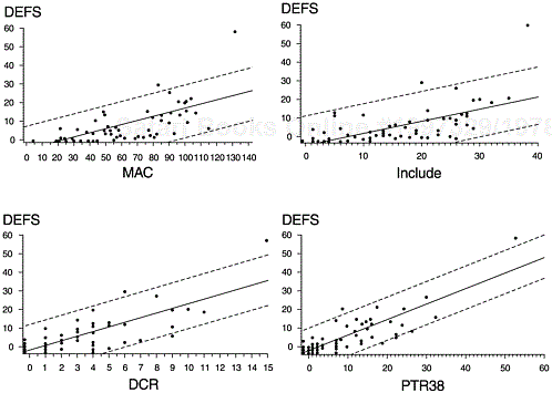
The extreme data point at the upper right corner of the diagrams represents the best known module in the component, which formats a display of messages in a queue and sends it to either the screen or printer. With more than 5,000 lines of source code, it is a highly complex module with a history of many problems.
The next step in our analysis was to look at the combined effect of these metrics on defect level simultaneously. To achieve this task, we used the multiple regression approach. In a multiple regression model, the effect of each independent variable is adjusted for the effects of other variables. In other words, the regression coefficient and the significance level of an independent variable represent the net effect of that variable on the dependent variable—in this case, the defect level. We found that in the combined model, MAC and INCLUDE become insignificant. When we excluded them from the model, we obtained the following:
With an R2 of 0.83, the model is highly significant. Each of the three independent variables is also significant at the 0.05 level. In other words, the model explains 83% of the variations in defect level observed among the program modules.
To verify the findings, we must control for the effect of program size—lines of code. Since LOC is correlated with DEFS and other variables, its effect must be partialled out in order to conclude that there are genuine influences of PTR38, DCR, and CPX on DEFS. To accomplish the task, we did two things: (1) normalized the defect level by LOC and used defects per KLOC (DEFR) as the dependent variable and (2) included LOC as one of the independent variables (control variable) in the multiple regression model. We found that with this control, PTR38, DCR, and CPX were still significant at the 0.1 level. In other words, these factors truly represent something for which the length of the modules cannot account. However, the R2 of the model was only 0.20. We contend that this again is due to the wide fluctuation of the dependent variable, the defect rate. The regression coefficients, their standard errors, t values, and the significance levels are shown in Table 11.5.
This analysis indicates that other than module length, the three most important factors affecting the defect rates of the modules are the number of changes and enhancements, defect history, and complexity level. From the intervention standpoint, since developers have no control over release enhancements, the latter two factors become the best clues for quality improvement actions. The relationships among defect history, complexity, and current defect level are illustrated in Figure 11.4. The best return on investment, then, is to concentrate efforts on modules with high defect history (chronic problem modules) and high complexity.
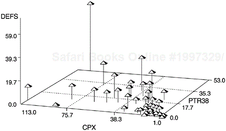
Table 11.5. Results of Multiple Regression Model of Defect Rate
|
Variable |
Regression Coefficients |
Standard Error |
t Value |
Significance (p Value) |
|---|---|---|---|---|
|
Intercept |
4.631 |
2.813 |
1.65 |
.10 |
|
CPX |
.115 |
.066 |
1.73 |
.09 |
|
DCR |
1.108 |
.561 |
1.98 |
.05 |
|
PTR38 |
.359 |
.220 |
1.63 |
.10 |
|
LOC |
–.014 |
.005 |
2.99 |
.004 |
|
R2 |
.20 |
Based on the findings from this analysis and other observations, the component team established a quality improvement plan with staged implementation. The following list includes some of the actions related to this analysis:
Scrutinize the several modules with moderate complexity and yet high defect level. Examine module design and code implementation and take proper actions.
Identify high-complexity and chronic problem modules, do intramodule restructuring and cleanup (e.g., better separation of mainline and subroutines, better comments, better documentation in the prologue, removal of dead code, better structure of source statements). The first-stage target is to reduce the complexity of these modules to 35 or lower.
Closely related to the preceding actions, to reduce the number of compilation warning messages to zero for all modules.
Include complexity as a key factor in new module design, with the maximum not to exceed 35.
Improve test effectiveness, especially for complex modules. Use test coverage measurement tools to ensure that such modules are adequately covered.
Improve component documentation and education.
Since the preceding analysis was conducted, the component team has been making consistent improvements according to its quality plan. Field data from new releases indicate significant improvement in the component’s quality.
This chapter describes several major metrics and models with regard to software module and design from the viewpoint of the metrics’ correlation with defect level. Regardless of whether the metrics are lines of code, the software science metrics, cyclomatic complexity, other syntactic constructs, or structure metrics, these metrics seem to be operational definitions of the complexity of the software design and module implementation. In retrospect, the key to achieving good quality is to reduce the complexity of software design and implementation, given a problem domain for which the software is to provide a solution.
The criteria for evaluation of complexity metrics and models, therefore, rest on their explanatory power and applicability. Explanatory power refers to the model’s ability to explain the relationships among complexity, quality, and other programming and design parameters. Applicability refers to the degree to which the models and metrics can be applied by software engineers to improve their work in design, coding, and testing. This is related to whether the model or metric can provide clues that can lead to specific actions for improvement. As a secondary criterion to explanatory power, congruence between the underlying logic of the model and the reasoning patterns of software engineers also plays a significant role. As a case in point, McCabe’s complexity metrics may appeal more to programming development professionals than Halstead’s token-based software science. During the design, code, and test phases, software engineers’ line of reasoning is determined more in terms of decision points, branches, and paths than in terms of the number of operators and operands.
Like software reliability models, perhaps even more so, the validity of complexity metrics and models often depends on the product, the development team, and the development environment. Therefore, one should always be very careful when generalizing findings from specific studies. In this regard, the concept and approach of local software quality metrics seem quite appealing. Specific improvement actions, therefore should be based on pertinent empirical relationships.