6
Norm-Oriented Formulations
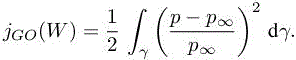
The previous chapters describe two important approaches for anisotropic mesh adaptation for PDEs, namely the feature-based approach and the goal-oriented approach. This chapter presents a third approach, the norm-oriented approach. The norm-oriented formulation extends the goal-oriented formulation since it is equation-based and uses an adjoint. At the same time, the norm-oriented formulation somewhat supersedes the goal-oriented approach since it is basically a solution-convergent method. Indeed, goal-oriented methods solely rely on the reduction of the error in evaluating a chosen scalar output with the consequence that, as mesh size is increased (more degrees of freedom), only this output is proven to tend to its continuous analog while the solution field itself may not converge. A remarkable quality of goal-oriented metric-based adaptation is the mathematical formulation of the mesh adaptation problem under the form of the optimization, in the well-identified set of metrics, of a well-defined functional. With the norm-oriented approach, this latter advantage is amplified by searching in the same well-identified set of metrics, the minimum of a norm of the approximation error. This norm then converges to zero when mesh size is increased. The type of norm is prescribed by the user and the method also addresses the case of multi-objective adaptation like, for example, in aerodynamics, adaptating the mesh for drag, lift and moment in one shot. Numerical examples for the Poisson problem and compressible flows are used for demonstrating the method.
6.1. Introduction
Goal-oriented methods have strongly impacted mesh adaptation applications. However, due to its formulation, a goal-oriented method has two inherent limitations. First, it does not naturally extend to several scalar outputs. This “multi-target” issue (explained in the sequel) is well known and a proposition for addressing it is made in Hartman (2008). Second, since the goal-oriented method is specialized to a given scalar output, the features of the solution field that are not influencing this output might be neglected by the automatic mesh improvement. A goal-oriented method provides the convergence of the approximate chosen output to its continuous analog. But generally, convergence does not hold for the whole flow field itself. To clarify this point, let us consider the mesh adaptative computation of a sonic boom footprint at the ground as presented in section 4.6.1 of this volume. The functional depends only on the pressure at the ground level. Now, many details of the flow on the upper part of the aircraft do not influence the pressure at the ground level. This vanishing influence is taken into account by the adjoint state, which also vanishes on these upper regions. Then, in these regions, the adapted mesh is not refined and the approximation of the flow field does not converge when the prescribed mesh size is increased. Another limitation of a goal-oriented method is related to the scalar character of the output to be best approximated. It leads to the use of integrals of solution fields for example (u − uh, g), u being the exact solution, uh its approximation and g a field prescribed by the user. Now, these integrals are generally not sufficiently sensitive to oscillating deviations between u and uh.
In the norm-oriented approach, the user can prescribe a semi-norm |u − uh| of the error, which will be minimized with respect to the mesh. If the semi-norm is also a norm, then the method allows the convergence of the unknown field. Among the possible choice of semi-norm, this can be the sum of square deviations of approximations of particular outputs. Let us take an example in aerodynamics. Let us assume that we wish to build the mesh that minimizes at the same time the errors on lift, drag and moment coefficients measured from flow solution uh. A direct goal-oriented method will rely on a weighted sum as functional j = α1CL(u)+ α2CD(u) + α3CM(u) and minimizing the error in the evaluation of j is prone to compensation between errors committed on these three aerodynamic coefficients since when we have made δj = α1(CL(u) − CL(uh)) + α2(CD(u) − CD(uh))+ α3(CM(u) − CM(uh)) small with an adhoc mesh, we cannot guarantee that the error on each of the three coefficients is small. A way to escape this default is to have three different functionals, with three adjoint states, to apply a necessary synthesis between the three mesh adaption solutions, which results in a notably increased computational cost. In contrast, minimizing the semi-norm ![]()
![]() will account for simultaneously minimizing the errors on lift, drag and moment measured from flow solution uh with respect to mesh. Returning to the sonic boom example of section 4.6.1, good results were obtained by minimizing the error on the functional [4.18]:
will account for simultaneously minimizing the errors on lift, drag and moment measured from flow solution uh with respect to mesh. Returning to the sonic boom example of section 4.6.1, good results were obtained by minimizing the error on the functional [4.18]:
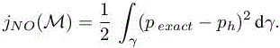
Instead of minimizing with respect to the metric the error |jGO(W) − jGO(Wh)| on this functional, it can be safer to minimize1 the actual deviation of the pressure itself:
In both above examples, we have chosen solely a semi-norm of the deviation to exact of the global flow field W, and therefore we do not have convergence of W when mesh is refined.
The norm-oriented method potentially addresses any kind of norm or semi-norm, with the limitation that, as for the goal-oriented method, choosing a non-admissible observation of the state system must be avoided. See Arian and Salas (1999) for this notion. As for the goal-oriented method, the norm-oriented method takes into account the PDE features and, contrary to the goal-oriented method, in the case where a norm is prescribed, it produces an approximate solution field that does converge to the exact one in this norm.
The norm-oriented method is a rather general method extending to complex CFD models, but the discussion here will be developed with the example of a 2D Poisson problem discretized by the usual linear finite-element method. This choice is motivated first by the rather complete set of theoretical works available for the finite-element approximation of a Poisson problem. This amount of theoretical background reduces as much as possible, although far from completely, the heuristics used in building the mesh adaptation analysis. A second motivation is the easy availability of exact solutions defined in a simple way. This allows us to build a kind of benchmark allowing to compare mesh adaptation methods. Let us mention also that the Poisson problem with variable coefficient is a central equation in two-fluid incompressible models as in Chapter 1 of Volume 1.
Although the usual FEM formulation relies on a projection in the H1 norm (with first-order convergence in H1), the user may wish to enjoy a convergence with a different norm. In this chapter, we consider the L2 norm, which provides second-order accuracy, but the method is stated in a sufficiently general way to allow extension to many types of norms or semi-norms. The method relies on the use of a corrector field as defined in Chapter 1 of this volume and on an a priori error estimate similar to the goal-oriented method (Chapter 4 of this volume) from which is extracted the asymptotically largest terms of the local error. This allows us to minimize the norm of the synthetic error computed with the corrector. In numerical experiments, in order to evaluate the validity of the synthetic error, we compare it with the one computed with the exact solution. Although theoretical convergence results (in which functional spaces?) are not available for Euler equations, the method can be extended to this CFD model and numerical illustrations will also be given.
Section 6.2 is devoted to a reformulation of the two above-identified mesh adaptation formulations: feature-based formulation as in Chapter 5 of Volume 1, and goal-oriented formulation as in Chapter 4 of this volume. In section 6.3, we present the norm-oriented mesh adaptation method. Section 6.4 is devoted to a numerical comparison between the two field-convergent formulations, namely, Hessian-based and norm-oriented. A CFD example is then discussed.
6.2. A summary of previous analyses
The feature-based analysis of Chapter 5 of Volume 1, the error estimate and goal-oriented analysis of Chapter 4 of this volume and the corrector derivations of Chapter 1 of this volume are shortly recalled in an abstract continuous context.
6.2.1. Feature-based adaptation by interpolation error optimization
Let u be any sufficiently smooth function defined on Ω, which we assume in this chapter to be in ℝ2. Let M be a metric of Ω. Metric M plays the role of the mesh and index M is used as indicating the approximate function uM by opposition to the exact one u. We consider metrics M parameterizing meshes sufficiently fine for justifying the replacement of the complete approximation error by its main asymptotic part. In particular, the P 1 interpolation error |ΠMu − u| on any mesh parameterized by the metric M can be represented by the continuous interpolation error defined in Chapter 3 of Volume 1:
where |Hu| is deduced from the Hessian of u, Hu, by taking the absolute values of its eigenvalues. The functional to minimize is

under the constraint that the complexity C(M) of the metric is equal to N. According to section 4.4 of Volume 1 (adapted to ℝ2), we get the unique optimal (MLp(x))x∈Ω as follows:
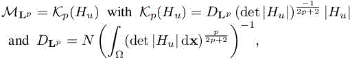
where ![]() is a global normalization term set to obtain a continuous metric with complexity N and
is a global normalization term set to obtain a continuous metric with complexity N and ![]() is a local normalization term accounting for the sensitivity of the Lp norm.
is a local normalization term accounting for the sensitivity of the Lp norm.
6.2.2. Implicit a priori error estimate and corrector
We are now considering the solution of an elliptic model
where ρ is a given strictly positive, bounded and possibly discontinuous field. Prescribing a complexity N of the metric M, we consider a still continuous approximation of [6.1] written as follows:
Equation [6.2] is an abstract equation representing with smooth ingredients any approximate of [6.1] built with any unit mesh H = HM of the metric M:
The implicit a priori error system [1.10] is then written
where Tij are the triangles of a unit mesh H for M.
We cannot completely transpose this system to a purely continuous one. We introduce an a priori corrector as introduced in section 1.2.2:
6.2.3. Goal-oriented analysis
This section recalls in an abstract formulation the application of goal-oriented analysis to the Poisson problem as presented in Chapter 5 of this volume. We minimize the error δjgoal(M) done when evaluating of the scalar output j =(g, u). This error is simplified as follows:
Let us define the adjoint state ![]() :
:
Then
and, using the analog of [1.8],

thus
Recall that u is unknown. The second term ![]() similar to the main term of the Hessian-based adaptation in section 6.2.1, can be explicitly approached in the same way, that is, introducing the continuous interpolation error defined in corollary 4.1 of Chapter 4 of Volume 1. It is the same for f:
similar to the main term of the Hessian-based adaptation in section 6.2.1, can be explicitly approached in the same way, that is, introducing the continuous interpolation error defined in corollary 4.1 of Chapter 4 of Volume 1. It is the same for f:
For the remaining ![]() term, we first apply lemma 5.1 and also use the continuous interpolation error πM. We get
term, we first apply lemma 5.1 and also use the continuous interpolation error πM. We get
Finally, the goal-oriented optimal metric problem is defined as follows:
When we change the parameter M, the discrete adjoint ![]() is close to its (non-zero) continuous limit and is thus not much affected, in contrast to the interpolation errors
is close to its (non-zero) continuous limit and is thus not much affected, in contrast to the interpolation errors ![]() We then consider, for a given M0, the following auxiliary optimum problem:
We then consider, for a given M0, the following auxiliary optimum problem:

Expressing as in Chapter 3 of Volume 1 the abstract interpolation errors in terms of the metric M, this will produce an optimum:
Observing that, in the integrand,

is a positive symmetric matrix, we can apply the above calculus of variation and get

where K1 is defined in [6.1]. This solution can then be introduced in a fixed-point loop and will produce the solution of

6.3. Norm-oriented approach
We are now interested by the minimization of the following expression with respect to the mesh M:
Introducing ![]() we get a formulation similar to the goal-oriented formulation:
we get a formulation similar to the goal-oriented formulation:
Let us define the discrete adjoint state ![]() :
:
Then, similarly to section 6.2.3, we have to solve the following optimum problem:

Exactly as for section 6.2.3, we freeze the dependency of the adjoint state.


In this analysis, we have frozen gM = u − uM. This term is unknown and the norm-oriented principle is to replace it by a good and not computationally costly corrector. We use the corrector ![]() defined in section 6.2.2. The gM RHS in [6.4]–[6.5] is replaced by
defined in section 6.2.2. The gM RHS in [6.4]–[6.5] is replaced by ![]() The dependency of the corrector with respect to the mesh will be solved in the outer fixed loop as in section 6.2.3. In order to get the final norm-oriented optimum Mopt,norm, we finish the computation as in Algorithm 4.1 of this volume.
The dependency of the corrector with respect to the mesh will be solved in the outer fixed loop as in section 6.2.3. In order to get the final norm-oriented optimum Mopt,norm, we finish the computation as in Algorithm 4.1 of this volume.
The norm-oriented method presented in Algorithm 6.1. involves the solution of two extra linear systems with respect to a basic feature-based algorithm and one extra linear system with respect to a goal-oriented algorithm.
REMARK 6.1.– In contrast to the adjoint of the goal-oriented algorithm, the two auxiliary variables uprio,M and ![]() are not consistent with a continuous adjoint and do not converge toward it when mesh is refined. They are correctors and converge to zero. A special strategy needs to be applied for solving then in a full-multigrid formulation (see Brèthes and Dervieux 2016). □
are not consistent with a continuous adjoint and do not converge toward it when mesh is refined. They are correctors and converge to zero. A special strategy needs to be applied for solving then in a full-multigrid formulation (see Brèthes and Dervieux 2016). □
6.4. Numerical elliptic examples
The method is first demonstrated with two Poisson problems in 2D. We compare the two mesh adaptation methods that produce L2 convergent solutions to continuous:
– the feature-based method with p =2 in section 6.2.1;
– the norm-oriented method directly built on the minimization of the L2 error norm.
We do not consider goal-oriented applications that we consider as being not convergent for the solution field.
6.4.1. Numerical features
In Brèthes et al. (2015), a mesh-adaptative full-multigrid (AFMG) algorithm relying on the Hessian-based adaptation criterion is proposed. We first describe in short this algorithm for the Hessian-based option. A sequence of numbers Nk of vertices is specified from a coarse mesh to finer one N0 = N,N1 = 4N, N2 =16N, N3 = 64N, .... For each mesh size Nk, a sequence of adapted meshes of size Nk is built by iterating the following loop:
a) computing a solution;
b) computing the optimal metric;
c) building the adapted mesh.
Algorithm 6.1. Norm-oriented mesh adaptation for a steady problem
In (a), a multi-grid V-cycle is applied to a sufficient convergence. In (b), approximations of the Hessians are performed as in Chapter 5 of Volume 1. While changing the mesh, an interpolation is applied in order to enjoy a good initial condition. A prescribed number of four adaptation iterations are applied at each mesh fineness Nk.
The extension of the above loop to norm-oriented adaptation consists of replacing the single Hessian evaluation by:
– the computation of the corrector, using MG and, as initial solution, the previous evaluation interpolated to current mesh2;
– the computation of the adjoint, using MG and, as initial solution, the previous evaluation interpolated to current mesh3;
– the evaluation of [6.8].
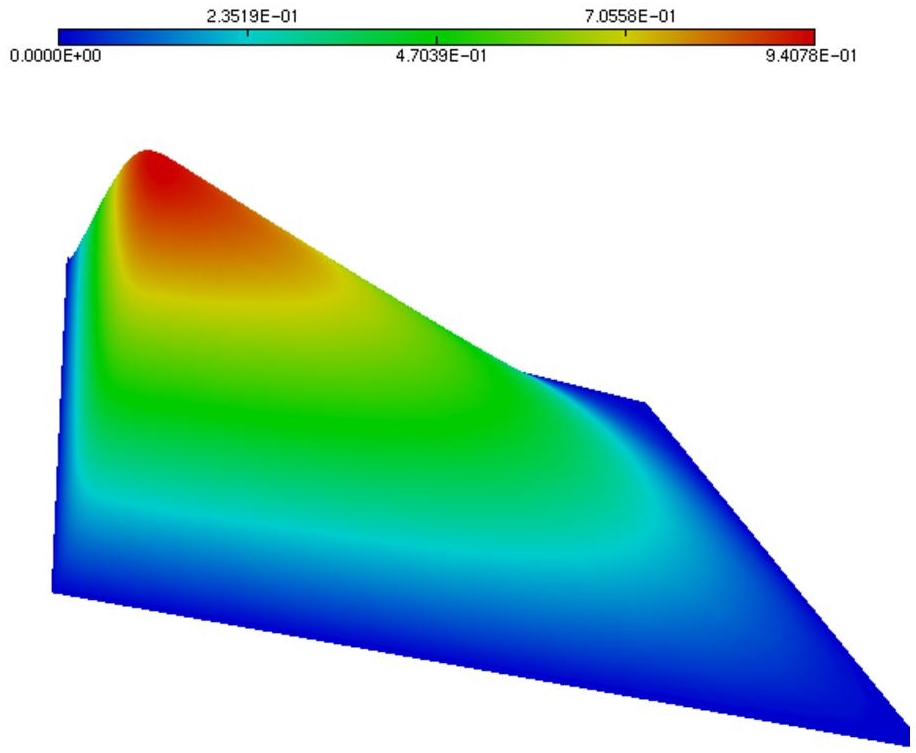
Figure 6.1. Fully 2D boundary layer test case: sketch of the solution. For a color version of this figure, see www.iste.co.uk/dervieux/meshadaptation2
Let us discuss computer efficiency. In the demonstrator of Brèthes et al. (2015), a particular feature is the stopping criterion of FMG that applies to the convergence of the solution of the unique solved system, that is, the system under study, u = A−1f. It is then possible to enjoy a better initial condition and control the iterative and approximation errors convergence. Consequently, it was possible, in Brèthes et al. (2015), to show that mesh adaptation carries large improvement not only in terms of accuracy for a given number of vertices but also in terms of accuracy for a given computational time. In contrast, the method proposed in this paper involves three systems to solve: (1) the system under study, u = A−1f, (2) the corrector system and (3) the adjoint system. We shall give an idea of the performances for one test case.
6.4.2. 2D boundary layer
This test case was proposed in Formaggia and Perotto (2003). Details of the calculation presented here can be found in Brèthes and Dervieux (2016). We solve the Poisson problem −Δu = f in ]0, 1[×]0, 1[ with Dirichlet boundary conditions and a right-hand side f chosen for having:
The coefficient α is chosen equal to 100. The graph of the solution is depicted in Figure 6.1. Before applying our mesh adaptative algorithm, it is interesting to evaluate the accuracy of our correctors. We choose a 161 × 161 uniform mesh and show in Figure 6.2 the cut of u− uh compared with the cut of both options of corrector u′. We observe that the a priori corrector does its job in a correct but inaccurate manner, while the DC one is rather accurate. We have also observed that the DC corrector does not consume notably more CPU than the a priori one. Therefore, we keep the DC option for the rest of the test case.
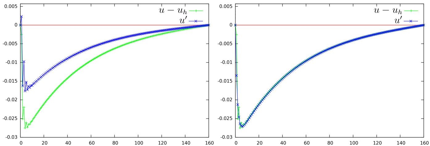
Figure 6.2. Fully 2D boundary layer test case. Left: Comparison of the a priori corrector  with approximation error u − uh (+), error cuts for y = 0.5. The a priori corrector is able to correct about 60% of the approximation error amplitude. Right: Comparison of the defect-correction corrector
  with the approximation error (+), error cuts for y = 0.5. The defect-correction corrector is able to correct about 95% of the amplitude. For a color version of this figure, see www.iste.co.uk/dervieux/meshadaptation2
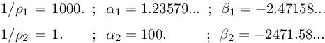
In Figure 6.3, we show a set of FMG calculations for the considered test case. The numbers of vertices of the successive meshes are supported by the horizontal axis, from 120 vertices to 30,000 vertices. The vertical axis gives the L2-norm of the approximation error |u − uh|L2 obtained on the mesh. Its variation with respect to number of vertices is compared in Figure 6.3 for the three following algorithms: (a) the uniform-mesh FMG, (b) the Hessian-based adaptative FMG and (c) the norm-oriented adaptative FMG. We observe that both adaptation methods carry an important improvement with respect to uniform-grid FMG (25,921 vertices on the finest mesh). For essentially the same number of vertices (32,318), the Hessian option gives an error divided by 47. The norm-oriented option appears as better with an error divided by 208 with 29,485 vertices. Since the exact solution u is analytically available, we could check that replacing the corrector by u − uh gives a very close convergence, in fact not better (see Brèthes and Dervieux 2016).
6.4.3. Poisson problem with discontinuous coefficient
This test case (also detailed in Brèthes and Dervieux 2016) exemplifies the singularity, which is met in the simulation of multi-fluid flows with a large deviation between the two values of the density, ρ1 and ρ2, uniform in each phase. In the case where a projection algorithm is applied to solve the Navier–Stokes equations for incompressible flow, a Poisson problem with discontinuous coefficients has to be solved as shown in section 1.3 of Volume 1. The present case does not satisfy the smoothness assumptions introduced for deriving our method, but the usual expectation in mesh adaptation is that the method also applies to non-smooth contexts. We consider the equation of Poisson ![]() with a discontinuous coefficient taking two different values 1/ρ1 and 1/ρ2 on two sub-domains Ω1 and Ω2 separated by an interface, which is a sufficiently smooth curve for having a normal vector. This PDE is mathematically referred as a transmission problem and the solution is continuous across the interface but of discontinuous normal derivatives since 1/ρ1 ∇u1 · n =1/ρ2∇u2 · n, where u1 and u2 are the restrictions of the solution u on Ω1 and Ω2. In our example, we define them as u|Ωi = ui = αi + βi(x2 + y2) i =1, 2. Further, Ω2 is the disk of center (0.5, 0.5) and radius 0.2 in the computational domain ]0, 1[×]0, 1[ and we have
with a discontinuous coefficient taking two different values 1/ρ1 and 1/ρ2 on two sub-domains Ω1 and Ω2 separated by an interface, which is a sufficiently smooth curve for having a normal vector. This PDE is mathematically referred as a transmission problem and the solution is continuous across the interface but of discontinuous normal derivatives since 1/ρ1 ∇u1 · n =1/ρ2∇u2 · n, where u1 and u2 are the restrictions of the solution u on Ω1 and Ω2. In our example, we define them as u|Ωi = ui = αi + βi(x2 + y2) i =1, 2. Further, Ω2 is the disk of center (0.5, 0.5) and radius 0.2 in the computational domain ]0, 1[×]0, 1[ and we have
This is sketched in Figure 6.4.
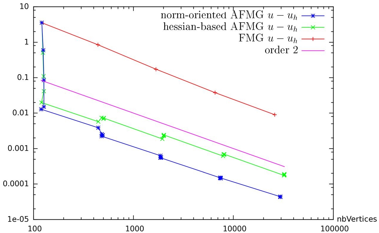
Figure 6.3. Fully 2D boundary layer test case: convergence of the error norm |u−uh|L2 as a function of number of vertices in the mesh for (+) non-adaptative FMG, (×) Hessian-based adaptative FMG and (∗) norm-oriented adaptative FMG. The quasi-vertical segments at abscissa nbV ertices ≈ 128 corresponds to the error reduction by the anisotropic mesh adaptation at constant complexity (i.e. quasi-constant number of vertices). These quasi-vertical segments corresponding to anisotropic adaptation phases also appear (less clearly) for abscissae nbV ertices ≈ 512, 2048, 8196. Oblique segments correspond to phases in which all the elements of the mesh are purely divided in four subelements by using mid-edges. As can be expected, the mesh division produces a reduction of the error by a factor of four because of second-order convergence. In contrast, anisotropic adaptation produces a tremendous error reduction for 128 vertices and not so much for the higher number of vertices. Our interpretation of this is that the main detail, the boundary layer, involves a single scale, it thickness (no smaller detail exists inside the boundary layer or elsewhere), and once the mesh has taken into account this scale, no important further improvement is possible. A last remark is that the norm-oriented approach delivers a convergence order slightly better than two while the feature-based approach delivers a slightly degraded convergence for the finer mesh, confirming that the best mesh for interpolation is not the best mesh for approximation. For a color version of this figure, see www.iste.co.uk/dervieux/meshadaptation2
Our analysis for defining correctors uses intensively smoothness of functions and assumes, for the defect-correction option, that second-order convergence applies, which is not true for this discontinuous case. However, the injection of the correctors in the norm-oriented functional and adjoint performs adequately. The anisotropy of the finer mesh is illustrated in Figure 6.5. A convergence in terms of number of vertices with non-adaptative and Hessian-based adaptive is given in Figure 6.6. We observe that, without mesh adaptation (crosses +), the convergence order is around one. This behavior can be explained by the singularity of the solution. In contrast, the overall convergence order of the adaptative process is about two. Note that this convergence will finally deteriorate when we attain the limits of the stretching capabilities of the mesh generator. However, the second-order numerical convergence observed is a usual bonus obtained by anisotropic mesh adaptation, which has already been noted in Loseille et al. (2007). In Brèthes et al. (2015), the convergence of an anisotropic adaptation has been compared with its isotropic analogs for the same test case. The anisotropic calculation converges at order two, while the isotropic calculation converges at order 3/2. A short analysis of these behaviors is proposed in Chapter 2 of Volume 1 and in Courty et al. (2006).
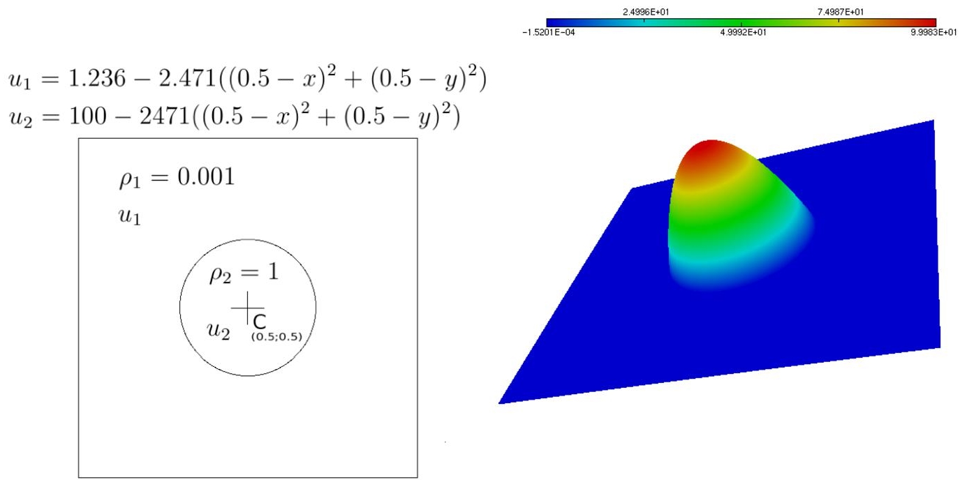
Figure 6.4. Poisson problem with discontinuous coefficient: sketch of exact solution definition and a typical computation of it. For a color version of this figure, see www.iste.co.uk/dervieux/meshadaptation2
Let us now compare with the feature-based method. This is the only one of our test cases for which the convergence of error in terms of number of nodes of the norm-oriented formulation is not neatly better (but it is as good) than the analog convergence of the feature-based formulation. Both adaptive algorithms give an error 10 times smaller than the non-adaptive one at a given time (Brèthes and Dervieux 2016).
Figure 6.5. Poisson problem with discontinuous coefficient. Views of final mesh (from left): global view, zoom on right part, zoom of the zoom
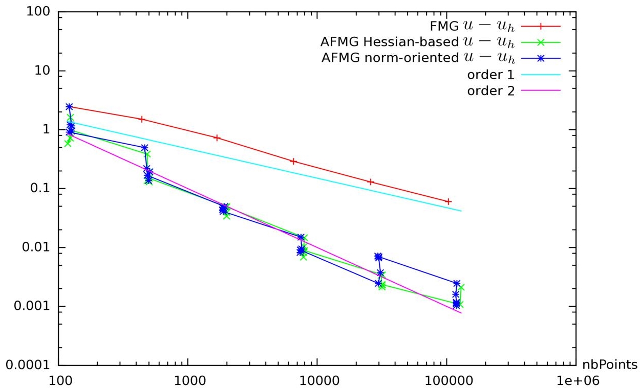
Figure 6.6. Poisson problem with discontinuous coefficient. Convergence of the error norm |u−uh|L2 as a function of number of vertices in the mesh for nonadaptative FMG (+), Hessian-based adaptative FMG (×) and norm-oriented adaptative FMG (∗). The non-adaptive convergence is solely a first-order one as expected for a singular solution. The two mesh-adaptation approaches produce second-order accuracy. Note that the mesh adaptation bonus appears in good part during the mesh enrichment phases. For a color version of this figure, see www.iste.co.uk/dervieux/meshadaptation2
6.5. Application to flows
The above method can be extended to insviscid and viscous compressible flows. It combines the analysis of the goal-oriented approach, as defined in Chapters 4 and 5 with the correctors for Euler and Navier–Stokes computed as in Chapter 1 and introduced as g functions in the goal-oriented estimate.
6.5.1. A comparison feature-oriented/norm
We consider the geometry provided for the first AIAA CFD High Lift Prediction Workshop (Configuration 1). We consider an inflow at Mach 0.2 with an angle of attack of 13◦. The flow model is Euler and final rather coarse meshes are used for a more clear comparison of the three adaptation strategies which are tested: the first one controls the interpolation error on the density, velocity and pressure in L1 norm, the second controls the interpolation error on the Mach number while the third one is based on the norm-oriented approach and controls the norm of the approximation error ||W − Wh||L2.
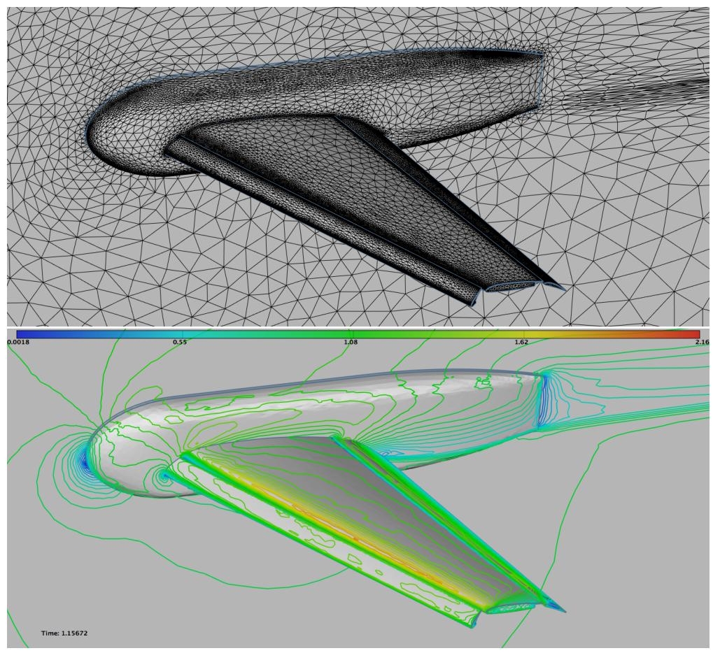
Figure 6.7. Feature-based adaptation for minimizing the L1 norm of the interpolation error on the density, velocity and pressure. Top: View of the skin mesh. There is not much mesh concentration on the body in the wake of wing. Bottom: Velocity on the aircraft skin. For a color version of this figure, see www.iste.co.uk/dervieux/meshadaptation2
For each case, five adaptations at fixed complexity are performed for a total of 15 adaptations with the following complexities: [160,000, 320,000, 640,000]. This choice leads to final meshes having around one million vertices. The residual for the flow solver convergence is set to 10−9 for each case. The generation of the anisotropic meshes is done with the local remeshing strategy of Loseille and Menier (2013). The surface meshes and the velocity iso-lines are depicted in Figures 6.7–6.9. Depending on the adaptation strategy, rather different flow fields are observed. The adaptation on the Mach number reveals strong shear layers at the wing tip that are not present in the norm-oriented approach. On the contrary, recirculating flows are observed on the norm-oriented approach while not being observed on the Mach number adaptation. For each case, the wakes have different features. Note that the accuracy near the body is not equivalent. For the L1 norm adaptation error and norm-oriented approaches, the far-field and inflow are much more refined than in the Mach number adaptation. This leads to better resolved phenomena for the final considered complexity. This example illustrates the need to control the whole flow field. Indeed, if the adaptation on the Mach number can provide a second-order convergent Mach number field, there is no guarantee on the other fields (density, pressure, velocity, etc.). In addition, the adaptation with the norm-oriented approach tends to increase the refinement at the inflow boundary condition and also at the far-field, although the interpolation error (on all variables) is negligible in these areas. Consequently, it seems of main interest to control all the sources of error, especially when the final intent is to certify a flow simulation.
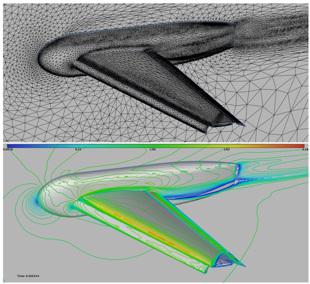
Figure 6.8. Feature-based adaptation for minimizing the L1 norm of the interpolation error on Mach number. Top: View of the skin mesh. There is not much mesh concentration on the body in the wake of wing. Bottom: Velocity on the aircraft skin. For a color version of this figure, see www.iste.co.uk/dervieux/meshadaptation2
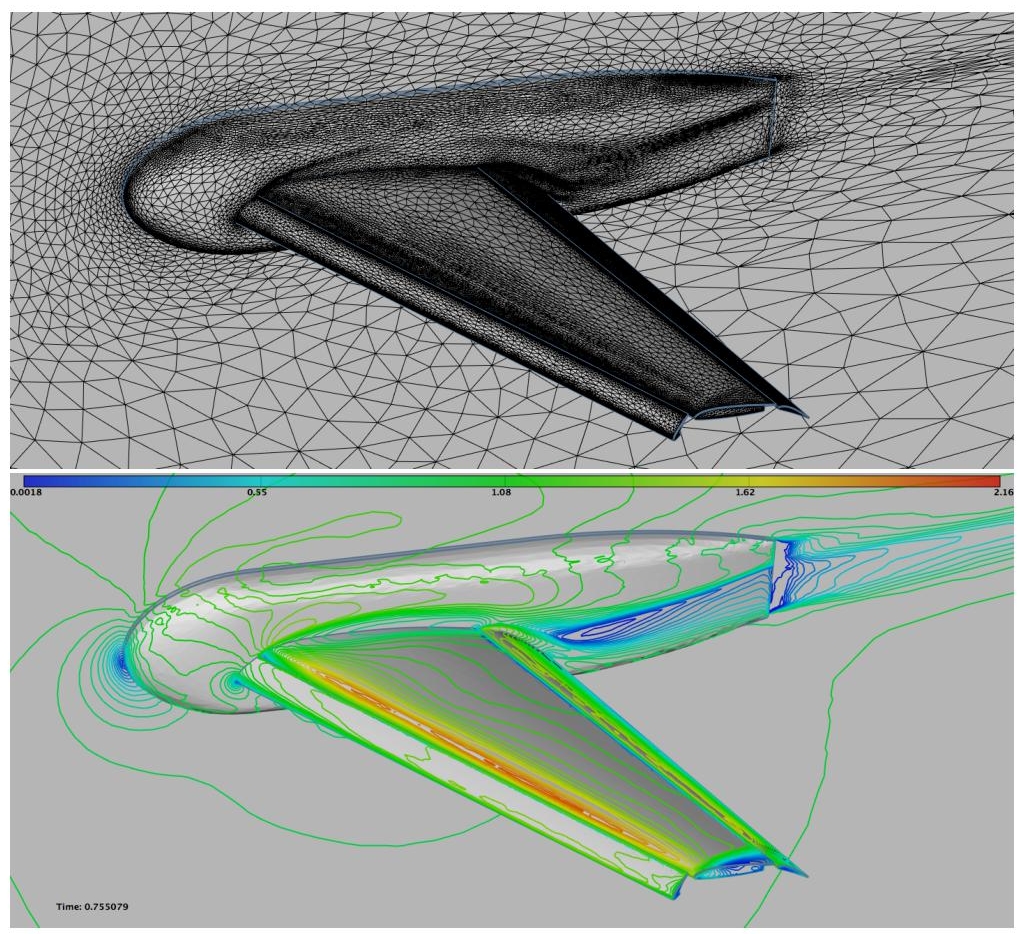
Figure 6.9. Adaptation for minimizing the norm ||W − Wh||L2 with the norm-oriented approach. Top: view of the skin mesh. Near-body mesh is finer and shows much more details on the aircraft body. Bottom: Velocity on the aircraft skin. For a color version of this figure, see www.iste.co.uk/dervieux/meshadaptation2
6.5.2. Application to a viscous flow
The last example is the flow around a Falcon aircraft, a test case from the UMRIDA program of European Union (see Alauzet et al. (2019)). The Mach number is 0.8, the angle of attack α =2 degrees and a Spalart–Allmaras turbulence model is used. The norm-oriented mesh adaptation is applied, except in a region close to boundary layer. In that region, a structured boundary layer mesh is kept frozen up to y+ = 500, while the mesh is solely adapted in the upper boundary layer region and the outer field. We choose to control the interpolation error on the local Mach number in L2 norm. Fifteen mesh adaptation iterations are performed. We split the adaptation loop into three phases with an increasing theoretical complexity (outside of the boundary layer region). Within each step, the adapted mesh at a fixed theoretical complexity is converged in five iterations. The final adapted meshes for each step contain 2,298,958, 6,168,815 and 10,337,483 vertices for theoretical complexities of, respectively, 100,000, 200,000 and 400,000. The final adapted mesh (for the largest complexity) is illustrated in Figure 6.10.
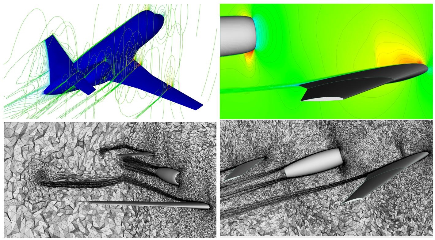
Figure 6.10. Top: Mach solution field. Bottom: final adapted mesh. Shape: courtesy of Dassault Aviation. For a color version of this figure, see www.iste.co.uk/dervieux/meshadaptation2
Such adapted meshes considerably enhance the efficiency of the flow solver and the solution accuracy. We first note that the wake is highly resolved and the wing tip vortices are well captured. Second, mesh refinements along the shock on the upper surface of the wing lead to an accurate computation of the shock – boundary layer interaction. We also observe a nice transition between the boundary layer structured mesh and the adapted anisotropic mesh.
6.6. Conclusion
The norm-oriented mesh adaptation method gives an answer to a well-formulated problem. Considering a numerical scheme and prescribing a norm, we want to find the mesh giving the smallest approximation error in that norm for a given number of vertices. The norm-oriented mesh adaptation method transforms the problem into an optimization problem, which is mathematically well-posed. It relies on the following other features.
A corrector represents the approximation error at the cost of a linearized state. In Chapter 1 of this volume, we give two examples of correctors for an elliptic model. An a priori corrector is built from the variational discrete statement. A defect-correction corrector is built from a finer-mesh defect correction principle. These correctors appear as not always very accurate but sufficiently accurate for our purpose. According to the type of approximation, at least the second one, defect-correction is extendable to many models and schemes.
The norm-oriented algorithm is presented as a natural extension of the goal-oriented algorithm which, in our formulation, is itself an extension of the Hessian-based algorithm. More precisely, while the Hessian-based algorithm solves only the PDE under study in the mesh-adaptation loop, the goal-oriented algorithm also solves an adjoint system (with linearized operator, transposed). The norm-oriented algorithm solves three systems, a corrector (linearized system with an adhoc RHS), an adjoint (linearized and transposed with the corrector as RHS) and the PDE itself. The three algorithms have in common an anisotropic a priori error analysis and a metric-based mesh parameterization. The feature-based method produces convergent solution fields but does not take into account the precise equation and discretization. The goal-oriented method takes into account equation and discretization but is too focused on a particular output and does not generally produce convergent solution fields. The norm-oriented method has the advantages of both.
6.7. Notes
Some other numerical examples are presented in Brèthes and Dervieux (2016).
Other approaches. Taking into account the influence of the PDE on the error through an equation-based estimate has been an important topic in the literature. The formulation of goal-oriented methods was an important step for a more justified error evaluation. It has been introduced in Becker and Rannacher (1996). It relied on an a posteriori estimate. A good synthesis concerning a posteriori estimates is given in Verfürth (2013); see also Ern and Vohralík (2015). An interest of a posteriori estimate is that it is expressed in terms of the approximate solution, assumed to be available in a mesh adaptation loop. A second interest is that it does not require the use of higher order (approximate) derivatives, in contrast to truncation analyses. These estimates show accurately where the mesh should be refined. A method for deducing a better anisotropic mesh from an a posteriori estimate, such as the one from Becker and Rannacher (1996), is proposed in Formaggia and Perotto (2003), while a theory for Hp norms in Agouzal and Vassilevski (2010) and a joint analysis of Hp and Lp norms of the error are presented in Agouzal et al. (2010). These methods cannot focus on an arbitrary user-specified error norm but relies on a particular one, specified by the variational formulation of the PDE. A more popular option is to choose, as accuracy target, a particular scalar output depending on the PDE solution. Any scalar output can be considered, except that difficulties can arise for the so-called non-admissible ones, according to Arian and Salas (1999). An a posteriori estimate also allows for building correctors for goal-oriented analyses (Giles and Pierce 1999; Pierce and Giles 2000). In Venditti and Darmofal (2000), the goal-oriented approach is cleverly combined with the correction strategy of Pierce and Giles (2000) and with the Hessian-based metric approach, still minimizing the interpolation error of a user-prescribed feature.